An Alternating Iteration Algorithm for a Parameter-Dependent Distributionally Robust Optimization Model

Abstract

Based on a successive convex programming method, an alternating iteration algorithm is proposed for solving a parameter-dependent distributionally robust optimization. Under the Slater-type condition, the convergence analysis of the algorithm is obtained. When the objective function is convex, a modified algorithm is proposed and a less-conservative solution is obtained. Lastly, some numerical tests results are illustrated to show the efficiency of the algorithm.

1. Introduction

In stochastic programming, the involved random variables usually satisfy certain distribution. However, in the real world, the certain distribution may be unknown or only the part of it is known. Distributionally robust optimization (DRO) method happens to be an effective way to solve such uncertain problems.

The study of the DRO method can be traced back to Scarf’s early work [1], which is intended to address potential uncertainties in supply chain and inventory control. In the DRO method, historical data may not be sufficient to estimate future distribution, therefore, a larger distribution set containing the true distribution can adequately address the risk of fuzzy uncertainty sets. The DRO model has been widely used in operations research, finance and management science, see [2,3,4,5,6] for recent development and further research. However, most of the ambiguity set of DRO are independent of decision variable.

Recently, Zhang, Xu and Zhang [7] have proposed a parameter-dependent DRO model, where the probability of the underlying random variables depends on the decision variables and the ambiguity set is defined through parametric moment conditions with generic cone constraints. Under Slater-type conditions, the quantitative stability results are established for the parameter-dependent DRO. By recent developments from the variational theory, Royset and Wets [8] have established convergence results for approximations of a class of DRO problems with decision-dependent ambiguity sets. Their discussion covers a variety of ambiguity sets, including moment-based and stochastic-dominance-based ones. Luo and Mehrotra [9] have obtained formulations for problems that feature distributional ambiguity sets defined by decision-dependent bounds on moments. Until recently, DRO with decision-dependent ambiguity sets has been an almost untouched research field. The few studies [7,8,9] on DRO with decision-dependent ambiguity sets are mostly theoretical achievements and the algorithms for solving such DRO are not related.

In this paper, for the parameter-dependent DRO model in [7], we propose an alternating iteration algorithm for solving it and propose a less-conservative solution strategy for its special case.

As far as we are concerned, the main contributions of this paper can be summarized as follows. Firstly, we carry out convergence analysis for alternating iteration algorithm. Under the Slater constraint qualification, we show that any cluster point of the sequence generated by the alternating iteration algorithm is an optimal solution of the parameter-dependent DRO. Notice that the proof of the convergence of successive convex programming method in [10] cannot cover our convergence analysis, since the uncertain set in Equation (1) depends on x, therefore our convergence analysis can be seen an extension of the proposition in [10]. Secondly, when the corresponding objective function is convex, a less-conservative DRO is constructed and a modified algorithm is proposed for it. At last, numerical experiments are carried out to show the efficiency of the algorithm.

The paper is organized as follows. Section 2 demonstrates the structure of the algorithm for the parameter-dependent DRO and establishes the convergence of the algorithm. In Section 3, the modified algorithm is proposed for a special case of DRO and the less-conservative solution is obtained. In Section 4, some numerical test results are illustrated to show the less conservative property of solutions obtained by the modified algorithm.

Throughout the paper, we use the following notations. By convention, we use ${\mathbf{R}}^{n\times n}$ and $S^{n\times n}$ to denote the space of all $n\times n$ matrices and symmetric matrices respectively. For matrix $A\in S^{n\times n}$, $A⪯0$ means that A is a negative semidefinite symmetric matrix, $\parallel x\parallel$ denotes the Euclidean norm of a vector x in ${\mathbf{R}}^n$. For a real-valued function $\phi :{\mathbf{R}}^n\to \mathbf{R}$, $\nabla \phi \left(x\right)$ denotes the gradient of $\phi$ at x.

2. DRO Model and Its Algorithm

Consider the following distributionally robust optimization (DRO) problem:

$$\begin{array}{c}\hfill \left(P\right)\begin{array}{cc}{\displaystyle \underset{x}{min}}& {\displaystyle \underset{P\in \mathcal{P}\left(x\right)}{sup}{\mathbb{E}}_P\left[f(x,\xi \left(\omega \right))\right]}\hfill \\ \mathrm{s}.\mathrm{t}.& x\in X,\hfill \end{array}\end{array}$$

(1)

where X is a compact set of ${\mathbf{R}}^n$, $f:{\mathbf{R}}^n\times {\mathbf{R}}^k\to \mathbf{R}$ is a continuously differentiability function, $\xi :\mathsf{\Omega }\to \Xi$ is a vector of random variables defined on probability space $(\mathsf{\Omega },\mathcal{F},P)$ with support set $\Xi \subset {\mathbf{R}}^k$, for fixed $x\in X$, $\mathcal{P}\left(x\right)$ is a set of distributions which contains the true probability distribution of random variable $\xi$, and ${\mathbb{E}}_P[·]$ denotes the expected value with respect to probability measure $P\in \mathcal{P}\left(x\right)$.

In this paper, we consider the case when $\mathcal{P}\left(x\right)$ is constructed through moment condition

$$\mathcal{P}\left(x\right):=\left\{P\in \mathcal{P}:{\mathbb{E}}_P\left[\mathsf{\Psi }(x,\xi \left(\omega \right))\right]\in \mathcal{K}\right\},$$

(2)

where $\mathsf{\Psi }$ is a random map which consists of vectors and/or matrices with measurable random components, and $\mathcal{P}$ denotes the set of all probability distributions/measures in the space $(\mathsf{\Omega },\mathcal{F})$ and $\mathcal{K}$ is a closed convex cone in a finite dimensional vector and/or matrix spaces. If we consider $(\Xi ,\mathcal{B})$ as a measurable space equipped with Borel sigma algebra $\mathcal{B}$, then $\mathcal{P}\left(x\right)$ may be viewed as a set of probability measures defined on $(\Xi ,\mathcal{B})$ induced by the random variate $\xi$. To ease notation, we will use $\xi$ to denote either the random vector $\xi \left(\omega \right)$ or an element of ${\mathbf{R}}^k$ depending on the context.

When $\Xi$ is a finite discrete set, that is, $\Xi =\{{\xi }_1,\cdots ,{\xi }_N\}$, for some N, (2) can be written as

$$\mathcal{P}\left(x\right)=\left\{(p_1,\cdots ,p_N):\sum _{j=1}^N{p}_j\mathsf{\Psi }(x,{\xi }_j)\in \mathcal{K},p_j\ge 0,\sum _{j=1}^N{p}_j=1\right\}.$$

(3)

In this section, we consider the DRO model (1) with $\mathcal{P}\left(x\right)$ defined by (3). In this case,

$${\mathbb{E}}_P\left[f(x,\xi \left(\omega \right))\right]=\sum _{j=1}^N{p}_{j}f(x,{\xi }_j)and{\mathbb{E}}_P\left[\mathsf{\Psi }(x,\xi \left(\omega \right))\right]=\sum _{j=1}^N{p}_j\mathsf{\Psi }(x,{\xi }_j).$$

In [10], a successive convex programming (SCP) method for a max–min problem with fixed compact set is proposed. However, the SCP method in [10] cannot be used to solve (1) directly, since $\mathcal{P}\left(x\right)$ in (1) depends on x.

Based on the SCP algorithm, we propose an alternating iteration algorithm for solving (1). In the algorithm proposed, the optimal solution is obtained by alternative iteration of solutions of inner maximum problems and outer minimum problems in (1). For convenience, let

$$\mathcal{C}=\left\{(p_1,\cdots ,p_N)\in {\mathbf{R}}^N:p_j\ge 0,j=1,2,\cdots ,N,\sum _{j=1}^N{p}_j=1\right\}.$$

We know from the algorithm that if the algorithm stops in finite steps with ${\mathcal{C}}_{k+1}={\mathcal{C}}_k$ or $v_k\le t_k$, then $x_k$ is an optimal solution of (1). In practice, problem (6) can be solved by its dual problem. In the case when an infinite sequence is produced, we use the following theorem to ensure the validity of the algorithm.

We introduce a notation, which is used in the proof of the convergence of the Algorithm in

Table 1. The Alternating Iteration Algorithm.

1. Set $k=0$ and ${\mathcal{C}}_0=\left\{\widehat{P}\right\}$ with $\widehat{P}\in \mathcal{C}$ satisfying $\{x\in X:{\mathbb{E}}_{\widehat{P}}\left[\mathsf{\Psi }(x,\xi )\right]\in \mathcal{K}\}\ne \varnothing$.

2. Solve the outer problem $$\begin{array}{cc}{\displaystyle \underset{x,t}{min}}& t\hfill \\ \mathrm{s}.\mathrm{t}.& {\mathbb{E}}_P\left[f(x,\xi \left(\omega \right))\right]\le t,\forall P\in {\mathcal{P}}_k\left(x\right)\hfill \\ & x\in X,\hfill \end{array}$$ (6) and obtain the solution $(x_k,t_k)$, where ${\mathcal{P}}_k\left(x\right)=\{P\in {\mathcal{C}}_k:{\mathbb{E}}_P\left[\mathsf{\Psi }(x,\xi )\right]\in \mathcal{K}\}.$

3. Solve the inner problem $$\begin{array}{cc}{\displaystyle \underset{P}{max}}& {\mathbb{E}}_P\left[f(x_k,\xi )\right]\hfill \\ \mathrm{s}.\mathrm{t}.& {\mathbb{E}}_P\left[\mathsf{\Psi }(x_k,\xi )\right]\in \mathcal{K},\forall P\in \mathcal{C}\hfill \end{array}$$ (7) and obtain the solution ${\widehat{P}}_k$ and the optimal value $v_k$.

4. Let ${\mathcal{C}}_{k+1}={\mathcal{C}}_k\cup \left\{{\widehat{P}}_k\right\}$.

5. If ${\mathcal{C}}_{k+1}={\mathcal{C}}_k$ or $v_k\le t_k$, then a solution of (1) is found and the algorithm stops. Otherwise set $k=k+1$ and goto 2.

. Let $P,Q\in \mathcal{P}$, the total variation metric between P and Q is defined as (see, e.g., page 270 in [11]),

$$d_{TV}(P,Q):=\underset{h\in \mathcal{H}}{sup}\left|{\mathbb{E}}_P\left[h\left(\xi \right)\right]-{\mathbb{E}}_Q\left[h\left(\xi \right)\right]\right|,$$

(4)

where,

$$\mathcal{H}:=\left\{h:{\mathbf{R}}^k\to \mathbf{R}:his\mathcal{B}\mathrm{measurable},\underset{\xi \in \Xi }{sup}\left|h\left(\xi \right)\right|\le 1\right\},$$

(5)

Using the total variation norm, we can define the distance from a metric $P\in \mathcal{P}$ to a metric set $\mathcal{P}\subset \mathcal{P}$, that is,

$$d_{TV}(Q,\mathcal{P}):=\underset{P\in \mathcal{P}}{inf}{d}_{TV}(Q,P).$$

We next provide the convergence of the Algorithm in Table 1.

Theorem 1.

Let $\left\{x_n\right\}$ be a sequence generated by Algorithm in Table 1 and $x_0$ be a cluster point. If (a) $(x,P)\mapsto {\mathbb{E}}_P\left[f(x,\xi )\right]$ and $(x,P)\mapsto {\mathbb{E}}_P\left[\mathsf{\Psi }(x,\xi )\right]$ are both continuous on $X\times \mathcal{C}$, (b) for $x\in X,f(x,·)$ and $\mathsf{\Psi }(x,·)$ are finite valued and continuous on Ξ, (b) $0\in int\{{\mathbb{E}}_P\left[\mathsf{\Psi }(x_0,\xi )\right]-\mathcal{K}:P\in \mathcal{C}\}$, then $x_0$ is an optimal solution of problem (1).

Proof. 

Since ${\mathcal{C}}_n$ is an increasing sequence of sets and $\mathcal{C}$ is a compact set, we have ${lim}_{n\to \infty }{\mathcal{C}}_n$$=\mathrm{cl}\left[{\cup }_{n=1}^{\infty }{\mathcal{C}}_n\right]:={\mathcal{C}}^{+}.$ Since $x_0$ is a cluster point of $\left\{x_n\right\}$, there exists an subsequence of $\left\{x_n\right\}$ converging to $x_0$. Without loss of generality, for simplicity, we assume that $x_0$ is the limit point of $\left\{x_n\right\}$. We know from step 2 in the algorithm that $x_n$ is an optimal solution of

$$\begin{array}{cc}{\displaystyle \underset{x}{min}}& {\displaystyle \underset{P\in \mathcal{P}\left(x\right)\cap {\mathcal{C}}_n}{sup}{\mathbb{E}}_P\left[f(x,\xi \left(\omega \right))\right]}\hfill \\ \mathrm{s}.\mathrm{t}.& x\in X.\hfill \end{array}$$

(8)

Let ${\widehat{S}}_n\left(x\right)$ and ${\widehat{v}}_n\left(x\right)$ denote the optimal solution set and optimal value of

$$\underset{P\in {\mathcal{P}}_n\left(x\right)}{sup},{\mathbb{E}}_P\left[f(x,\xi )\right]$$

respectively, $\widehat{S}\left(x\right)$ and $\widehat{v}\left(x\right)$ denote the optimal solution set and optimal value of

$$\underset{P\in \mathcal{P}\left(x\right)\cap {\mathcal{C}}^{+}}{sup}{\mathbb{E}}_P\left[f(x,\xi )\right],$$

respectively. Then, we have from (8) that:

$${\widehat{v}}_n\left(x_n\right)\le {\widehat{v}}_n\left(x\right)\mathrm{for}\mathrm{any}x\in X.$$

(9)

We proceed the rest of the proof in three steps.

Step 1. We next show

$$\underset{n\to \infty }{lim}{\widehat{v}}_n\left(x_n\right)=\widehat{v}\left(x_0\right).$$

(10)

Let ${\widehat{P}}_n\in {\widehat{S}}_n\left(x_n\right)$, by compactness of ${\mathcal{C}}^{+}$, $\left\{{\widehat{P}}_n\right\}$ has cluster points. We assume ${\widehat{P}}^{*}$ is a cluster point of $\left\{{\widehat{P}}_n\right\}$, then there exists a subsequence $\left\{n_k\right\}\subseteq \left\{n\right\}$ such that ${\widehat{P}}_{n_k}$ converges to ${\widehat{P}}^{*}$ weakly as $k\to \infty$ and ${\widehat{P}}^{*}\in {\mathcal{C}}^{+}$. Under conditions (a) and (b), we have

$${\widehat{v}}_{n_k}\left(x_{n_k}\right)={\mathbb{E}}_{{\widehat{P}}_{n_k}}\left[f(x_{n_k},\xi )\right]\to {\mathbb{E}}_{{\widehat{P}}^{*}}\left[f(x_0,\xi )\right]\le \widehat{v}\left(x_0\right)$$

as $k\to \infty$. Hence, we have

$$\underset{n\to \infty }{lim\; sup}{\widehat{v}}_n\left(x_n\right)\le \widehat{v}\left(x_0\right).$$

(11)

Since ${\mathcal{P}}_n\left(x_n\right)=\mathcal{P}\left(x_n\right)\cap {\mathcal{C}}_n\ne \varnothing$, we have form condition (a) that $\mathcal{P}\left(x_0\right)\cap {\mathcal{C}}^{+}\ne \varnothing$, which means that $\widehat{S}\left(x_0\right)\ne \varnothing$. Let $P^{*}\in \widehat{S}\left(x_0\right)$, we next show that there exists a sequence $\left\{{\widehat{P}}_n\right\}$ with ${\widehat{P}}_n\in {\mathcal{P}}_n\left(x_n\right)$ such that ${\widehat{P}}_n$ converges to $P^{*}$ weakly as $n\to \infty$. Under conditions (b) and (c), we know from [Theorem 2.1] in [7] that there exist positive constants $\gamma$ and $\nu \in (0,1)$ such that:

$$d_{TV}(Q,\mathcal{P}\left(x_n\right))\le \gamma {\parallel x_n-x_0\parallel }^{\nu }$$

for all $Q\in \mathcal{P}\left(x_0\right)$ and n large enough, which means that for $P^{*}\in \widehat{S}\left(x_0\right)$,

$$d_{TV}(P^{*},\mathcal{P}\left(x_n\right)\cap {\mathcal{C}}_n)\le d_{TV}(P^{*},\mathcal{P}\left(x_n\right))+d_{TV}(P^{*},{\mathcal{C}}_n)\le \gamma {\parallel x_n-x_0\parallel }^{\nu }+d_{TV}(P^{*},{\mathcal{C}}_n)$$

(12)

for n large enough. Let ${\widehat{P}}_n={\mathsf{\Pi }}_{\mathcal{P}\left(x_n\right)\cap {\mathcal{C}}_n}\left(P^{*}\right)$, then by (12), we have ${\widehat{P}}_n$ converges to $P^{*}$ weakly as n converges to infinity. Consequently, under condition (b),

$${\widehat{v}}_n\left(x_n\right)\ge {\mathbb{E}}_{{\widehat{P}}_n}\left[f(x_n,\xi )\right]\to {\mathbb{E}}_{P^{*}}\left[f(x_0,\xi )\right]=\widehat{v}\left(x_0\right)$$

as $n\to \infty$ and hence,

$$\underset{n\to \infty }{lim\; inf}\widehat{v}\left(x_n\right)\ge \widehat{v}\left(x_0\right).$$

(13)

Combining (11) and (13), we have $\widehat{v}\left(x_n\right)$ converges to $\widehat{v}\left(x_0\right)$ as $n\to \infty$.

Step 2. We next show for any fixed $x\in X$,

$$\underset{n\to \infty }{lim}{\widehat{v}}_n\left(x\right)=\widehat{v}\left(x\right).$$

(14)

Since ${lim}_{n\to \infty }{\mathcal{C}}_n={\mathcal{C}}^{+}$, we have ${lim}_{n\to \infty }\mathcal{P}\left(x\right)\cap {\mathcal{C}}_n=\mathcal{P}\left(x\right)\cap {\mathcal{C}}^{+}$.

Then under conditions (a) and (b), similarly to the proof of step 1, we have ${\widehat{v}}_n\left(x\right)$ converges to $\widehat{v}\left(x\right)$ as $n\to \infty .$

Step 3. Combining (9), (10) and (14), we have

$$\widehat{v}\left(x_0\right)\le \widehat{v}\left(x\right)\mathrm{for}\mathrm{any}x\in X,$$

(15)

which means that, $x_0$ is an optimal solution of

$$\begin{array}{cc}{\displaystyle \underset{x}{min}}& {\displaystyle \underset{P\in \mathcal{P}\left(x\right)\cap {\mathcal{C}}^{+}}{sup}{\mathbb{E}}_P\left[f(x,\xi \left(\omega \right))\right]}\hfill \\ \mathrm{s}.\mathrm{t}.& x\in X.\hfill \end{array}$$

(16)

By step 3 in algorithm, we have

$$\underset{P\in \mathcal{P}\left(x_n\right)\cap {\mathcal{C}}^{+}}{sup}{\mathbb{E}}_P\left[f(x_n,\xi )\right]\le \underset{P\in \mathcal{P}\left(x_n\right)\cap \mathcal{C}}{sup}{\mathbb{E}}_P\left[f(x_n,\xi )\right]={\mathbb{E}}_{{\widehat{P}}_{n+1}}\left[f(x_n,\xi )\right]\le \underset{P\in \mathcal{P}\left(x_n\right)\cap {\mathcal{C}}^{+}}{sup}{\mathbb{E}}_P\left[f(x_n,\xi )\right],$$

which means that

$$\underset{P\in \mathcal{P}\left(x_n\right)\cap {\mathcal{C}}^{+}}{sup}{\mathbb{E}}_P\left[f(x_n,\xi )\right]=\underset{P\in \mathcal{P}\left(x_n\right)\cap \mathcal{C}}{sup}{\mathbb{E}}_P\left[f(x_n,\xi )\right].$$

Then by the proof in step 1, letting $n\to \infty$, we have $\widehat{v}\left(x_0\right)={sup}_{P\in \mathcal{P}\left(x_0\right)\cap \mathcal{C}}{\mathbb{E}}_P\left[f(x_0,\xi )\right].$ Consequently, by (15), we have

$$\widehat{v}\left(x_0\right)\le \widehat{v}\left(x\right)\le \underset{P\in \mathcal{P}\left(x\right)\cap \mathcal{C}}{sup}{\mathbb{E}}_P\left[f(x,\xi )\right]$$

for all $x\in X$. Therefore, $x_0$ is an optimal solution of (1). □

Remark 1.

In [10], without any constraint qualifications, the proof of the convergence of SCP method is obtained. However, in our proof, since the uncertain set in (1) depends on x, the Slater condition ensures the proof. We know from the above proof that if the uncertain set in (1) independent on x, the Slater condition can be omitted. Therefore our convergence analysis can be seen an extension of the proposition in [10].

3. Less Conservative Model and a Modified Algorithm

In this section, we consider a special case of (1) and provide a less-conservative model.

In the case when $\Xi =\{{\xi }_1,\cdots ,{\xi }_N\}$ and the ambiguity set is

$$\mathcal{P}\left(x\right):=\left\{P\in \mathcal{P}:\begin{array}{c}{\mathbb{E}}_P{[\xi -{\mu }_0]}^T{\Sigma }_0^{-1}{\mathbb{E}}_P[\xi -{\mu }_0]\le {\gamma }_1\\ {\mathbb{E}}_P\left[(\xi -{\mu }_0){(\xi -{\mu }_0)}^T\right]-{\gamma }_2{\Sigma }_0⪯0\end{array}\right\},$$

(17)

where ${\gamma }_1$ and ${\gamma }_2$ are nonnegative constants, ${\mu }_0\in {\mathbf{R}}^k$ and ${\Sigma }_0\in S^{k\times k}$ is positive semidefinite, the model (1) is the following problem:

$$\begin{array}{cc}\underset{x\in X}{min}\underset{(p_1,\cdots ,p_N)\in {\mathbf{R}}^N}{max}\hfill & {\mathbb{E}}_P\left[f(x,\xi )\right]\hfill \\ \mathrm{s}.\mathrm{t}.\hfill & \sum _{j=1}^N{p}_j{g}_1\left({\xi }_j\right)⪯0,\hfill \\ \hfill & \sum _{j=1}^N{p}_j{g}_2\left({\xi }_j\right)⪯0,\hfill \\ \hfill & p_j\ge 0,j=1,\cdots ,N,\hfill \\ \hfill & \sum _{j=1}^N{p}_j=1,\hfill \end{array}$$

(18)

where

$$g_1\left(\xi \right)=\left[\begin{array}{cc}-{\Sigma }_0& {\mu }_0-\xi \\ {({\mu }_0-\xi )}^T& -{\gamma }_1\end{array}\right]$$

and

$$g_2\left(\xi \right)=(\xi -{\mu }_0){(\xi -{\mu }_0)}^T-{\gamma }_2{\Sigma }_0.$$

The model has been investigated in [2]. As shown in [2], the constraints in (18) imply that the mean of $\xi$ lies in an ellipsoid of size ${\gamma }_1$ centered at the estimate ${\mu }_0$ and the centered second moment matrix of $\xi$ lies in a positive semidefinite cone defined with a matrix inequality.

However, in the constraints of (18), not all ${\xi }_j$ lies in the ellipsoid of size ${\gamma }_1$ centered at the estimate ${\mu }_0$. In practice, we may be only interested in the ${\xi }_j$ which lies in the ellipsoid and omit the ones outside the ellipsoid. Consequently, we propose a less-conservative DRO model, that is

$$\begin{array}{cc}\underset{x\in X}{min}\underset{(p_1,\cdots ,p_N)\in {\mathbf{R}}^N}{max}\hfill & {\mathbb{E}}_P\left[f(x,\xi )\right]\hfill \\ \mathrm{s}.\mathrm{t}.\hfill & p_j{g}_1\left({\xi }_j\right)⪯0,\hfill \\ \hfill & p_j{g}_2\left({\xi }_j\right)⪯0,\hfill \\ \hfill & p_j\ge 0,j=1,\cdots ,N,\hfill \\ \hfill & \sum _{j=1}^N{p}_j=1.\hfill \end{array}$$

(19)

In the above model, if the ${\xi }_j$ does not lie in an ellipsoid of size ${\gamma }_1$ centered at the estimate ${\mu }_0$ or does not satisfy the matrix inequality $g_2\left({\xi }_j\right)⪯0$, the corresponding constraints are vanished. Moreover, we can choose ${\gamma }_1$ and ${\gamma }_2$ such the feasible set of the inner problem is not empty, for example, for the first constraint, let ${\gamma }_1=max\{{({\xi }_j-{\mu }_0)}^T{\Sigma }_0^{-1}({\xi }_j-{\mu }_0):j=1,2,\cdots ,N\}$. Compare with model (18), the model (19) is less conservative since the feasible set of the inner maximum problem is smaller.

Let $\mathcal{Q}$ be a set of probability distributions defined as

$$\mathcal{Q}=\left\{(p_1,\cdots ,p_N)\in {\mathbf{R}}^N:p_j{g}_i\left({\xi }_j\right)⪯0,\sum _{j=1}^N{p}_j=1,p_j\ge 0,j=1,\cdots ,N,i=1,2\right\}.$$

(20)

Next we give a modified alternative solution algorithm for (19):

The above algorithm is based on the algorithm in Pflug and Wozabal [10] for solving a distributed robust investment problem and a cutting plane algorithm in Kelley [12] for solving convex optimization problems. A similar algorithm has been used in Xu et al. [5] to solve a different DRO model and the proof of the convergence is omitted. In the following, we provide convergence analysis of the modified alternative solution algorithm based on Theorem 1.

Theorem 2.

Let $\left\{x_n\right\}$ be a sequence generated by Algorithm in

Table 2. The Modified Alternating Iteration Algorithm.

1. Let ${\mathbf{P}}_0=(p_1^0,\cdots ,p_N^0)\in \mathcal{Q}$ and ${\mathcal{Q}}_0:=\left\{{\mathbf{P}}_0\right\}$ and $x_0\in X$. Set $k=0$.

2. Solve the outer minimization problem $$\begin{array}{cc}\underset{x,t}{min}\hfill & t\hfill \\ \mathrm{s}.\mathrm{t}.\hfill & x\in X,\hfill \\ \hfill & \sum _{j=1}^N{p}_j^k[f(x_k,{\xi }_j)+{\nabla }_{x}f{(x_k,{\xi }_j)}^{\top }(x-x_k)]\le t,\mathrm{for}{\mathbf{P}}_k=(p_1^k,\cdots ,p_N^k)\in {\mathcal{Q}}_k\hfill \end{array}$$ (21) and obtain the solution $(x_{k+1},t_{k+1})$.

3. Solve the inner maximization problem $$\begin{array}{cc}\underset{(p_1,\cdots ,p_N)\in {\mathbf{R}}^N}{max}\hfill & \sum _{j=1}^N{p}_{j}f(x_{k+1},{\xi }_j)\hfill \\ \mathrm{s}.\mathrm{t}.\hfill & p_j\left[\begin{array}{cc}-{\Sigma }_0\hfill & {\displaystyle {\mu }_0-\xi }\hfill \\ {\displaystyle {({\mu }_0-\xi )}^{\top }}\hfill & -{\gamma }_1\hfill \end{array}\right]⪯0\hfill \\ \hfill & p_j\left[(\xi -{\mu }_0){(\xi -{\mu }_0)}^{\top }\right]⪯{\gamma }_2{\Sigma }_0,\hfill \\ \hfill & p_j\ge 0,j=1,\cdots ,N,\hfill \\ \hfill & \sum _{j=1}^N{p}_j=1\hfill \end{array}$$ (22) and obtain the solution $({\mathbf{P}}_{k+1},v_{k+1})$.

4. Let ${\mathcal{Q}}_{k+1}={\mathcal{Q}}_k\bigcup \left\{{\mathbf{P}}_{k+1}\right\}$. If ${\mathcal{Q}}_{k+1}={\mathcal{Q}}_k$ or $v_{k+1}\le t_{k+1}$, then stop, else let $k:=k+1$, go to 1.

and $x_0$ be a limit point. If for each $\xi \in \Xi$, $f(·,\xi )$ is continuously differentiable and convex on X, then $x_0$ is an optimal solution of problem (19).

Proof. 

The proof is similar as the proof of Theorem 1. Since ${\mathcal{Q}}_n$ is an increasing sequence of sets and $\mathcal{Q}$ is a compact set, we have ${lim}_{n\to \infty }{\mathcal{Q}}_n=\mathrm{cl}\left[{\cup }_{n=1}^{\infty }{\mathcal{Q}}_n\right]:={\mathcal{Q}}^{+}.$

Let ${\widehat{S}}_n\left(x\right)$ and ${\widehat{v}}_n\left(x\right)$ denote the optimal solution set and optimal value of

$$\underset{(p_1,\cdots ,p_N)\in {\mathcal{Q}}_n}{sup}\sum _{j=1}^N{p}_j[f(x_{n-1},{\xi }_j)+{\nabla }_{x}f{(x_{n-1},{\xi }_j)}^T(x-x_{n-1})]$$

respectively, $\widehat{S}\left(x\right)$ and $\widehat{v}\left(x\right)$ denote the optimal solution set and optimal value of

$$\underset{(p_1,\cdots ,p_N)\in {\mathcal{Q}}^{+}}{sup}\sum _{j=1}^N{p}_{j}f(x,{\xi }_j)$$

respectively. Then we have

$${\widehat{v}}_n\left(x_n\right)\le {\widehat{v}}_n\left(x\right)\mathrm{for}\mathrm{any}x\in X.$$

(23)

Let $(p_1^n,\cdots ,p_N^n)\in {\widehat{S}}_n\left(x_n\right)$, by compactness of ${\mathcal{Q}}^{+}$, $\left\{(p_1^n,\cdots ,p_N^n)\right\}$ has cluster points. We assume $(p_1^{*},\cdots ,p_N^{*})$ is a cluster point of $\left\{(p_1^n,\cdots ,p_N^n)\right\}$, then there exists a subsequence $\left\{n_k\right\}\subseteq \left\{n\right\}$ such that $(p_1^{n_k},\cdots ,p_N^{n_k})$ converges to $(p_1^{*},\cdots ,p_N^{*})$ weakly as $k\to \infty$ and $(p_1^{*},\cdots ,p_N^{*})\in {\mathcal{Q}}^{+}$. Then we have

$$\begin{array}{ccc}{\widehat{v}}_{n_k}\left(x_{n_k}\right)& =& \sum _{j=1}^N{p}_j^{n_k}[f(x_{n_k-1},{\xi }_j)+{\nabla }_{x}f{(x_{n_k-1},{\xi }_j)}^T(x_{n_k}-x_{n_k-1})]\hfill \\ & \le & \sum _{j=1}^N{p}_j^{n_k}f(x_{n_k},{\xi }_j)\to \sum _{j=1}^N{p}_j^{*}\left[f(x_0,{\xi }_j)\right]\le \widehat{v}\left(x_0\right)\hfill \end{array}$$

as $k\to \infty$. Hence, we have

$$\underset{n\to \infty }{lim\; sup}{\widehat{v}}_n\left(x_n\right)\le \widehat{v}\left(x_0\right).$$

(24)

On the other hand, for $(p_1^{*},\cdots ,p_N^{*})\in \widehat{S}\left(x_0\right),(p_1^{*},\cdots ,p_N^{*})\in {\mathcal{Q}}^{+}$, which means that $\exists (p_1^n,\cdots ,p_N^n)\in {\mathcal{Q}}^n$ such that

$$(p_1^n,\cdots ,p_N^n)\to (p_1^{*},\cdots ,p_N^{*})$$

as $n\to \infty$. Therefore, we have

$${\widehat{v}}_n\left(x_n\right)\ge \sum _{j=1}^N{p}_j^n[f(x_{n-1},{\xi }_j)+{\nabla }_{x}f{(x_{n-1},{\xi }_j)}^T(x_n-x_{n-1})]\to \sum _{j=1}^N{p}_j^{*}f(x_0,{\xi }_j)=\widehat{v}\left(x_0\right)$$

(25)

as $n\to \infty$. Combining (24) and (25), we obtain

$$\underset{n\to \infty }{lim}{\widehat{v}}_n\left(x_n\right)=\widehat{v}\left(x_0\right).$$

The else of proof follows from the proof of Theorem 1. □

Remark 2.

Notice that the Slater condition is not used in the proof, since the uncertain set in (1) is independent on x, the Slater condition can be omitted.

4. Numerical Tests

In this section, we discuss the numerical performance of proposed alternating iteration algorithm for solving (18) and (19). We do so by applying the alternating iteration algorithm to a news vender problem [4] and provide comparative analysis of the numerical results.

Suppose the company has to decide the order quantity $x_j$ of a product to meet the demand ${\xi }_j$ and the news provider trades in $j=1,\cdots ,n$ products. Before knowing the uncertain demand ${\xi }_j$, the news vender orders $x_j$ units of product j at the wholesale price $c_j>0$. Once the demand ${\xi }_j$ is known, it can be quantified $min\{x_j,\xi \}$ at the retail price of $v_j$. Any stock that have not been sold ${(x_j-{\xi }_j)}_{+}$ are cleared by the remedy price $h_j$. Any unsatisfied demand ${({\xi }_j-x_j)}_{+}$ is lost. The total loss of the news vendors can be described as a function of the order decision $x:={(x_1,\cdots ,x_n)}^{\top }$:

$$L(x,\xi )=c^{\top }x-v^{\top }min(x,\xi )-h^{\top }{(x-\xi )}_{+}={(c-v)}^{\top }x+{(v-h)}^{\top }{(x-\xi )}_{+},$$

(26)

where non-negativity and minimum operators are applied to the component method. We study the risk aversion of the news vendor problem on two models:

$$\begin{array}{c}\left(H1\right)\underset{x\in X}{min}\underset{P\in \mathcal{P}}{sup}{\mathbb{E}}_P\left[U\left(L(x,\xi )\right)\right],\hfill \end{array}$$

(27)

and

$$\begin{array}{c}\left(H2\right)\underset{x\in X}{min}\underset{P\in \mathcal{Q}}{sup}{\mathbb{E}}_P\left[U\left(L(x,\xi )\right)\right],\hfill \end{array}$$

(28)

where $U\left(w\right):=e^{w/10}$ is an exponential distribution function,

$$\mathcal{P}=\left\{(p_1,\cdots ,p_N)\in {\mathbf{R}}^N:\sum _{j=1}^N{p}_j{g}_i\left({\xi }_j\right)⪯0,\sum _{j=1}^N{p}_j=1,p_j\ge 0,j=1,\cdots ,N,i=1,2\right\}.$$

and $\mathcal{Q}$ is defined as in (20). Notice that for the news vender problem, problems (18) and (19) are just ($H1$) and ($H2$) respectively.

The data are generated as follows: for i-th product, wholesale, retail and remedy prices are $c_j=0.1(5+j-1)$, $v_j=0.15(5+j-1)$ and $h_j=0.05(5+j-1)$ respectively; the product demands vector $\xi$ is characterized by a multivariate log-normal distribution with the mean $\mu =({\mu }_1,\cdots ,{\mu }_n)$, ${\mu }_j=2,j=1,\cdots ,n.$ In the execution of the algorithm, we use an ambiguity set $\mathcal{Q}$ in (20) with ${\gamma }_1=0.1$ and ${\gamma }_2=1.1$. The mean and convariance matrix ${\mu }_0$ and ${\Sigma }_0$ are calculated to be generated through a computer. The experiments are carried out through Matlab 2016 installed on a Dell notebook computer with Windows 7 operating system and Intel Core i5 processor. The SDP subproblems in Algorithms are solved by Matlab solver “SDPT3-4.0” [13].

The computation results are shown in the

Table 3. The performance of ($H1$).

n	Time (s)	Iter	Optimal Value
2	31.234226	48	0.9669
4	44.774935	66	0.9663
6	52.961924	72	0.9616
8	52.583319	69	0.9578
10	56.231204	74	0.9659
12	65.792619	85	0.9629

and

Table 4. The performance of ($H2$).

n	Time (s)	Iter	Optimal Value
2	28.848998	48	0.9483
4	32.741311	50	0.7441
6	38.559070	57	0.7603
8	41.873316	57	0.8045
10	61.811460	76	0.8577
12	63.149645	75	0.8433

and Figure 1, Figure 2, Figure 3, Figure 4 and Figure 5 below sequentially. In Table 3 and Table 4, we show the average cpu time (Times(s)), iteration (Iter) and optimal values (Optimal Vlue) of each test problem with different sample sizes.

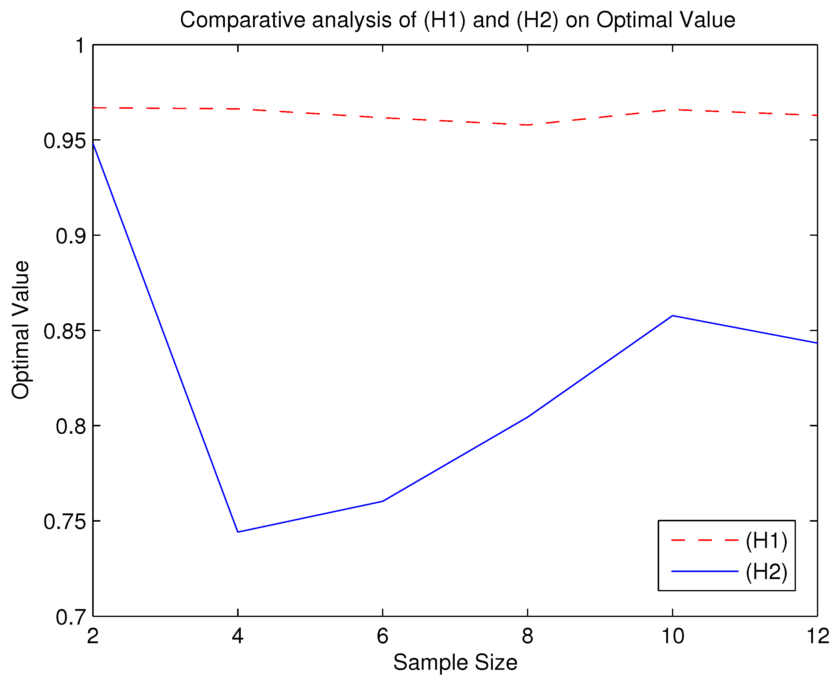
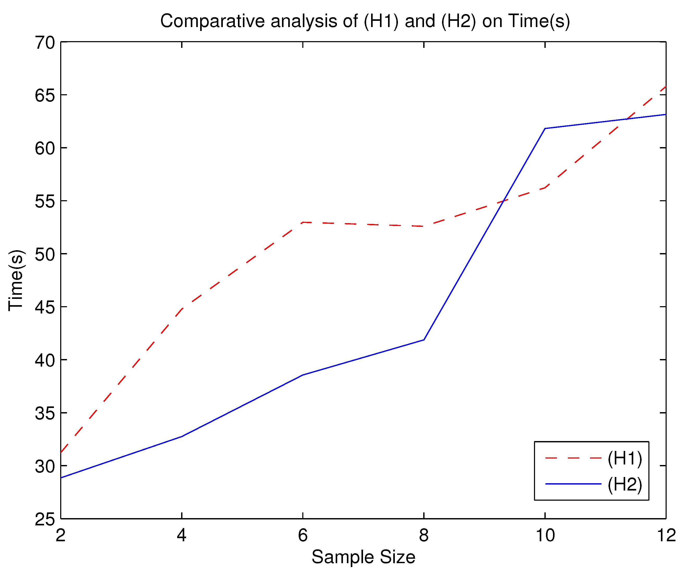
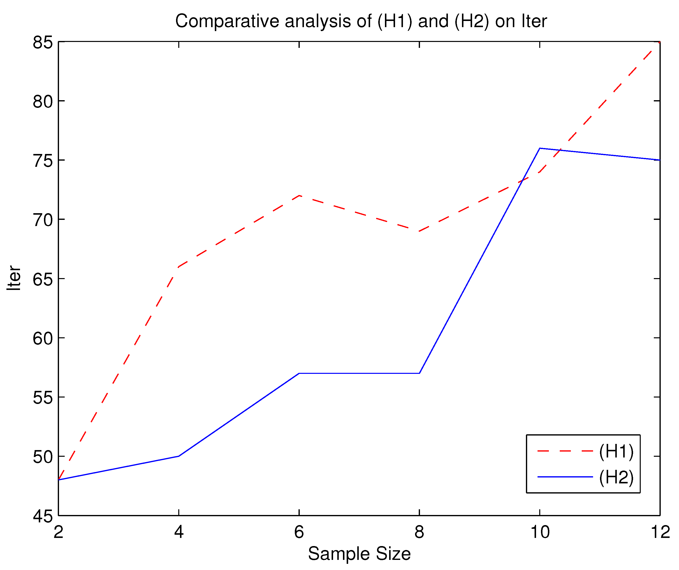
From the Table 3 and Table 4 and Figure 1, Figure 2, Figure 3, Figure 4 and Figure 5, we can roughly see that problems ($H1$) and ($H2$) can be solved by the alternating iteration algorithm. We know from Figure 1, Figure 2, Figure 3, Figure 4 and Figure 5 that when using the algorithm to solve ($H1$) and $\left(H2\right)$, the number of iterations and time of solving $\left(H1\right)$ are basically more than that of solving ($H2$). Moreover, the optimal values of $\left(H2\right)$ is smaller than the ones of ($H1$). Since the DRO model is usually used to describe an upper bound of uncertain optimization problems, the smaller the optimal value of the DRO model, the less conservative the DRO model is. 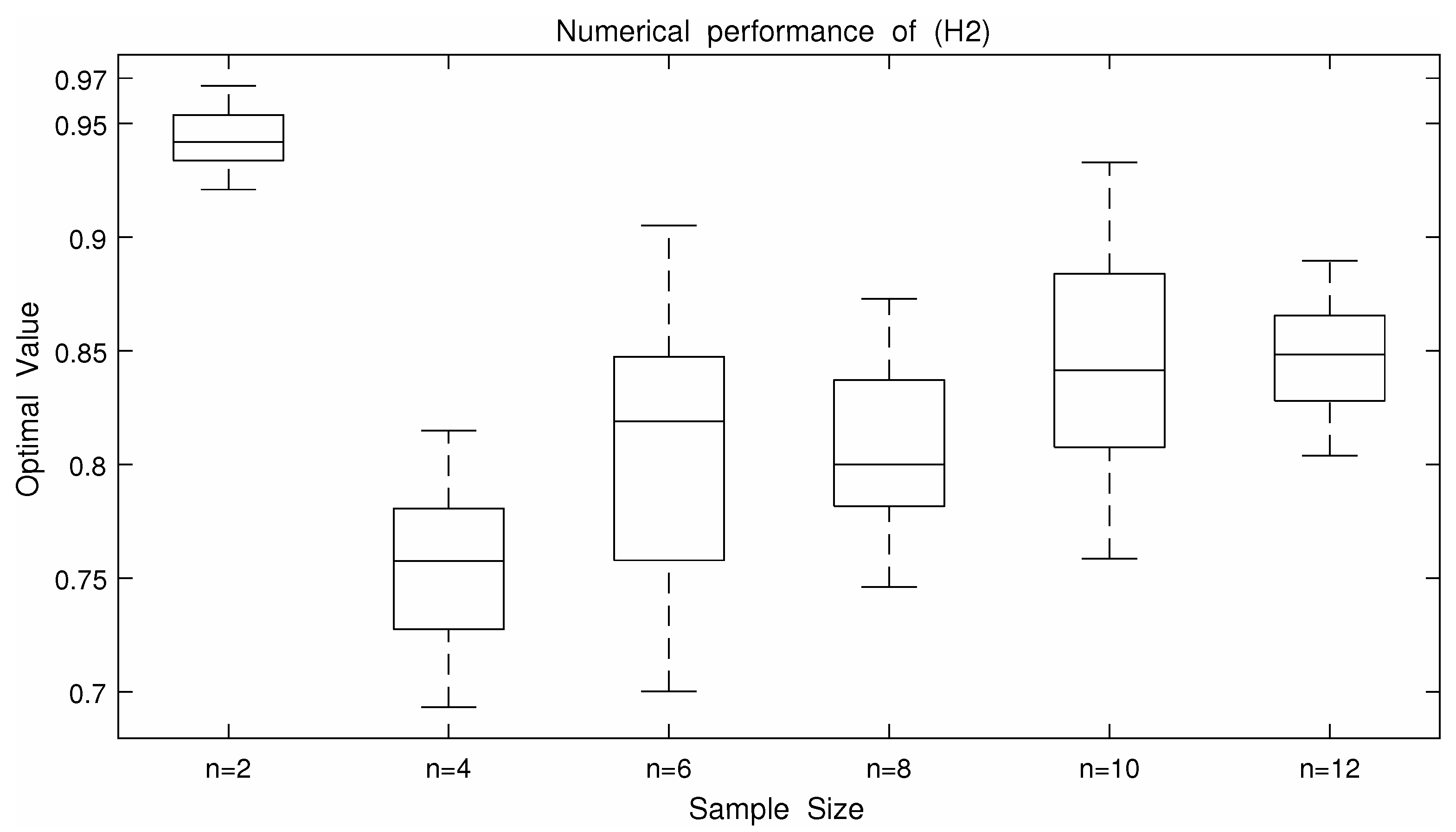Therefore, $\left(H2\right)$ is a less conservative DRO model. However, according to Figure 3, ($H1$) is more robust than $\left(H2\right)$ because the curve shown by ($H1$) is more stable.

The numerical results show that, in order to obtain a conservative total loss in the news vender problem, solving DRO model $\left(H2\right)$ by the alternating iteration algorithm usually performs better than solving DRO model $\left(H1\right)$. However, in our observations, when we only focus on the robustness, DRO model ($H1$) may be the better choice. We provide the links to the source codes as follows: https://pan.baidu.com/s/1dSmMUynZqi5LzWgn6aUUoQ?pwd=xn44 (accessed on 25 January 2022).

5. Conclusions

In this paper, we carry out convergence analysis for an alternating iteration algorithm for a distributionally robust optimization problem where the ambiguity set depends on decision variables. Convergence analysis of the alternating iteration algorithm are obtained under the Slater-type condition, which can be seen an extension of the result in [10]. When the objective function is convex, a modified alternating iteration algorithm is proposed for obtaining a less-conservative solution of DRO and the convergence analysis is established. Finally, we discuss the numerical performance of proposed alternating iteration algorithm for obtaining a conservative total loss in the news vender problem. We can undertake similar analysis when the ambiguity set in DRO is constructed in other ways such as Kullback–Leiblor divergence [14], Wasserstein metric [15,16] etc. We leave all these for future research as they are beyond the focus of this paper.