Proper ARMA Modeling and Forecasting in the Generalized Segre’s Quaternions Domain

Abstract

The analysis of time series in 4D commutative hypercomplex algebras is introduced. Firstly, generalized Segre’s quaternion (GSQ) random variables and signals are studied. Then, two concepts of properness are suggested and statistical tests to check if a GSQ random vector is proper or not are proposed. Further, a method to determine in which specific hypercomplex algebra is most likely to achieve, if possible, the properness properties is given. Next, both the linear estimation and prediction problems are studied in the GSQ domain. Finally, ARMA modeling and forecasting for proper GSQ time series are tackled. Experimental results show the superiority of the proposed approach over its counterpart in the Hamilton quaternion domain.

1. Introduction

Time series theory is a very well-known statistical methodology for the analysis of stochastic processes that has found widespread applications in signal processing, communications engineering, economics, astronomy, meteorology, seismology, oceanography, among other fields [1]. The most extensively used class of stationary process models are the so-called autoregressive moving average (ARMA) processes. The relevance of ARMA models stems from their power to approximate any stationary process arbitrarily well [2,3]. In addition, ARMA models can be cast in a state-space framework and also have enormous significance in prediction problems, since they facilitate the derivation of several efficient prediction algorithms [3].

The traditional settings for developing time series analysis have been the real and complex numbers, while other number systems have demonstrated a high potential to outperform them in some applications. The most paradigmatic example is the system of Hamilton quaternions (HQs), which has proven to be of great value for the description of 3-dimensional (3D) movements, in fields such as graphic design or automated control [4,5]. Actually, HQs have become the most popular and researched system of hypercomplex numbers [6]. In spite of its relevance, the use of this system in time series analysis is scarce [7].

HQs belong to a more general family of algebras, named hypercomplex systems, which extends the real and complex numbers to higher dimensions. Among them, 4D hypercomplex systems are of special relevance since four coordinates are usually considered for describing the physical world [6]. Further, depending on how the product is defined, they can be classified into two types: noncommutative and commutative systems. HQs are of the first type, i.e., they form a normed division algebra, and this property makes them well suited to deal with signal processing benchmark problems, such as the signal estimation problem [8]. Though commutative hypercomplex numbers, which includes the generalized Segre’s quaternions (GSQs), are less well known, their interest is increasing within the signal processing community due to their availability to extend the methodologies developed in the complex and real field to the 4D case [9,10,11,12,13,14,15,16,17,18,19,20,21]. These commutative hypercomplex algebras possess zero divisors, which implies that the Euclidean norm is not multiplicative [13]. This drawback, however, has essentially no impact on signal and image processing applications [10].

Interestingly, a recent line of research has discovered that the HQs algebra is not always the best option for processing 4D hypercomplex signals [22,23,24,25]. Specifically, some investigations have revealed that properness, a structural property of the hypercomplex signals, determines the performance of the used processing [24,25]. In all of these papers, the analyses have been performed by comparing HQs with tessarines, and several scenarios where the latter outperforms the former have been shown. It should be noted that tessarines are a subset of GSQs obtained by defining a particular product. In general, hypercomplex algebras are characterized by its product, which is usually provided by a multiplication table (Appendix A in [6]). From an intuitive point of view, it is to be expected that more general commutative hypercomplex algebras than tessarines can attain better performance results. On that basis, special attention is paid to such systems in this paper.

As indicated above, properness is a crucial property of hypercomplex signals. This property has two important effects: it determines which type of processing should be used, and also it achieves a significant decrease in the computational complexity involved in comparison to the real processing. Properness has been investigated in detail in the HQ domain [26,27,28,29,30], and for tessarines [24,25]. To our knowledge, however, properness has not been studied for GSQs yet.

Inspired by all the above discussed, the main objective of this paper is to present the time series analysis in the GSQs domain while analyzing the properness properties in this setting. Specifically, the concept of properness is introduced for GSQ signals and their properties studied. Remarkably, two tests to experimentally check whether real data are proper in the GSQs field are proposed and an estimate of the parameter characterizing the product in the hypercomplex algebra is provided. Such an estimate gives the best value of the parameter under which the properness properties could be fulfilled by the signal of interest. It should be highlighted that, unlike the existing approaches, a specific hypercomplex algebra is not fixed in advance in the proposed strategy, but a broad family of commutative hypercomplex algebras is considered. So, the suggested estimate allows us to select the particular algebra in which it is most likely to achieve, if possible, the properness properties. A simulation example illustrates how this approach is effective.

The linear estimation problem is also tackled. Although GSQ numbers are not a normed algebra and thus, the classical projection theorem cannot be applied to obtain the optimum linear estimate, we exploit its metric space feature to prove the existence and uniqueness of the projection and an extension of the innovations algorithm for proper GSQ signals is devised. As could be expected, the proposed algorithms attain a notable reduction in the computational burden. Finally, ARMA modeling for proper GSQ time series is introduced. For that, we first investigate an extension of the Yule–Walker equations and then, the prediction problem is addressed. The particular structure of the ARMA models allows us to improve the innovations algorithm giving rise to a more efficient prediction method. The steady-state properties of the suggested predictor are also studied. To conclude, the superiority in terms of performance of our proposal in comparison with its counterpart in the HQ domain is numerically analyzed.

The rest of this paper is organized as follows. Section 2 presents both the GSQ random variables and signals. Then, Section 3 introduces the concepts of properness in the GSQs domain and provides the statistical inference methods for testing the properness as well as estimating the associated parameter that characterizes the product in the hypercomplex algebra. This section ends with a simulation example. The linear estimation problem for GSQ random variables and the prediction problem for GSQ random signals are analyzed in Section 4. Section 5 focuses on the analysis of time series in the GSQs setting. It deals with the problems of modeling and forecasting time series data. A final example is included to show the efficiency of the proposed strategy. To improve the readability of the manuscript, all proofs have been deferred to Appendix B, Appendix C, Appendix D, Appendix E and Appendix F.

Notation

We designate matrices with boldface uppercase letters, column vectors with lowercase letters, and scalar quantities with lightface lowercase letters. Moreover, the symbols $\mathbb{Z}$, $\mathbb{R}$, $\mathbb{C}$, and $\mathbb{S}$ represent the set of integer, real, complex, and GSQ numbers, respectively. In this regard, $\mathbf{A}\in {\mathbb{R}}^{p\times q}$ (respectively, $\mathbf{A}\in {\mathbb{S}}^{p\times q}$) indicates that $\mathbf{A}$ is a real (respectively, a GSQ) matrix of dimension $p\times q$. Similarly $\mathbf{r}\in {\mathbb{R}}^p$ (respectively, $\mathbf{r}\in {\mathbb{S}}^p$) means that $\mathbf{r}$ is a p-dimensional real (respectively, a GSQ) vector. In particular, ${\mathbf{0}}_{p\times q}$ represents the zero matrix of dimension $p\times q$, and ${\mathbf{I}}_p$ is the identity matrix of dimension p. In addition, $A_{ij}$ denotes the $ij$ element of the matrix $\mathbf{A}$ and $diag(·)$ stands for a diagonal (or block diagonal) matrix with entries (or block entries) specified in the operator argument.

Furthermore, superscript “$\mathtt{T}$” represents the transpose. “⊗”stands for the Kronecker product. $E[·]$ represents the expectation operator. $\mathcal{R}\{·\}$ denotes the real part of a GSQ, and $\left|z\right|$ is either the complex modulus if $z\in \mathbb{C}$ or the absolute value if $z\in \mathbb{R}$. Finally, ${\delta }_{nl}$ denotes the Kronecker delta function.

Unless otherwise stated, all random variables are assumed to have a zero-mean throughout this paper.

A list of symbols that are used in the paper is given in Table 1.

Table 1. List of symbols.

Symbol	Meaning
${\mathbf{x}}_r\left(t\right)$	Real vector formed with the components of $\mathbf{x}\in {\mathbb{S}}^p$
$\overline{\mathbf{x}}\left(t\right)$	Augmented GSQ signal vector formed by $\mathbf{x}\in {\mathbb{S}}^p$ and its conjugations
${\mathsf{\Gamma }}_{\mathbf{a}}(t,s)$	Correlation function of a real random signal vector $\mathbf{a}\left(t\right)\in {\mathbb{R}}^p$
${\mathsf{\Gamma }}_{\mathbf{a}\mathbf{b}}(t,s)$	Correlation function of the real random signal vectors $\mathbf{a}\left(t\right)\in {\mathbb{R}}^p$ and $\mathbf{b}\left(t\right)\in {\mathbb{R}}^q$
${\mathsf{\Gamma }}_{\mathbf{x}}^{\nu }(\alpha ,t,s)$	$E\left[\mathbf{x}\left(t\right){\mathbf{x}}^{{\mathtt{H}}_{3-2\nu }}\left(s\right)\right]$, for $\mathbf{x}\in {\mathbb{S}}^p$, $\nu =1,2$
${\mathsf{\Gamma }}_{\mathbf{x}\mathbf{y}}^{\nu }(\alpha ,t,s)$	$E\left[\mathbf{x}\left(t\right){\mathbf{y}}^{{\mathtt{H}}_{3-2\nu }}\left(s\right)\right]$, for $\mathbf{x}\in {\mathbb{S}}^p$, $\mathbf{y}\in {\mathbb{S}}^q$, and $\nu =1,2$
${\mathsf{\Gamma }}_{\mathbf{x}}^3(\alpha ,t,s)$	$E\left[\mathbf{x}\left(t\right){\mathbf{x}}^{{\mathtt{H}}_{\alpha }}\left(s\right)\right]$, for $\mathbf{x}\in {\mathbb{S}}^p$
${\mathsf{\Gamma }}_{\mathbf{x}\mathbf{y}}^3(\alpha ,t,s)$	$E\left[\mathbf{x}\left(t\right){\mathbf{y}}^{{\mathtt{H}}_{\alpha }}\left(s\right)\right]$, for $\mathbf{x}\in {\mathbb{S}}^p$ and $\mathbf{y}\in {\mathbb{S}}^q$
${\widehat{\mathsf{\Gamma }}}_{\mathbf{x}}$	Sample autocorrelation matrix of a random vector $\mathbf{x}$
${\mathcal{C}}_{\alpha }$	Set of the random vectors $\{{\mathbf{x}}_1,\dots ,{\mathbf{x}}_m\}$, with ${\mathbf{x}}_i\in {\mathbb{S}}^p$, $i=1,\dots ,m$
${\overline{\mathcal{C}}}_{\alpha }$	Set of the augmented random vectors $\{{\overline{\mathbf{x}}}_1,\dots ,{\overline{\mathbf{x}}}_m\}$, with ${\overline{\mathbf{x}}}_i\in {\mathbb{S}}^{4p}$, $i=1,\dots ,m$
${\mathcal{G}}_{{\mathcal{C}}_{\alpha }}$	Set of all finite linear combinations of elements of ${\mathcal{C}}_{\alpha }$
${\mathcal{G}}_{{\overline{\mathcal{C}}}_{\alpha }}$	Set of all finite linear combinations of elements of ${\overline{\mathcal{C}}}_{\alpha }$
${\widehat{y}}^{\mathtt{SWL}}$	SWL estimator of y respect to ${\mathcal{C}}_{\alpha }$
${\widehat{y}}_{\alpha }^{\mathtt{S}}$	${\mathbb{S}}_{\alpha }$ estimator of y respect to ${\mathcal{C}}_{\alpha }$
${\widehat{y}}^{\mathtt{QSL}}$	QSL estimator of y respect to ${\mathcal{C}}_{\alpha }$
${ϵ}^{\mathtt{SWL}}$	SWL estimation error associated to ${\widehat{y}}^{\mathtt{SWL}}$
${ϵ}_{\alpha }^{\mathtt{S}}$	${\mathbb{S}}_{\alpha }$ estimation error associated to ${\widehat{y}}_{\alpha }^{\mathtt{S}}$
${ϵ}^{\mathtt{QSL}}$	QSL estimation error associated to ${\widehat{y}}^{\mathtt{QSL}}$

2. Generalized Segre’s Quaternion Random Variables

This section establishes the basic concepts and properties of interest in the GSQ domain. For that, we first introduce the GSQ random variables and then the GSQ random signals are considered.

A random variable $x\in \mathbb{S}$ can be defined as $x=a+\mathrm{i}b+\mathrm{j}c+\mathrm{k}d$ where $a,b,c,d\in \mathbb{R}$ are random variables and the imaginary units $(\mathrm{i},\mathrm{j},\mathrm{k})$ satisfy the following multiplication rules:

$$\begin{array}{c}\hfill \mathrm{ij}=\mathrm{k}, \mathrm{jk}=\mathrm{i}, \mathrm{ki}=\alpha \mathrm{j}, {\mathrm{i}}^2={\mathrm{k}}^2=\alpha , {\mathrm{j}}^2=1\end{array}$$

(1)

where $\alpha$ is a nonzero real number.

As is well-known, the form in which the product is defined is an essential feature of hypercomplex numbers. The product defined in (1) is commutative, associative, and distributive over addition; however, these algebras have divisors of zero. In contrast to GSQs, the product in the HQs is defined in such a way that the algebra becomes noncommutative and does not have divisors of zero [6]. Further, two special algebras in GSQs are of interest: for $\alpha >0$, $\mathbb{S}$ is called the hyperbolic quaternions system and for $\alpha <0$, $\mathbb{S}$ is the elliptic quaternions system [6]. In particular, if $\alpha =-1$ then, $\mathbb{S}$ is named the tessarine numbers.

The real vector of $x\in \mathbb{S}$ is defined by ${\mathbf{x}}_r={[a,b,c,d]}^{\mathtt{T}}$. Moreover, we define the following auxiliary GSQ random variables:

$$\begin{array}{cccc}\hfill x_{\alpha }& =a+\mathrm{i}\frac{b}{\alpha }+\mathrm{j}c+\mathrm{k}\frac{d}{\alpha }\hfill & \hfill & x^{\mathrm{i}}=a+\mathrm{i}b-\mathrm{j}c-\mathrm{k}d\hfill \\ \hfill x^{\mathrm{j}}& =a-\mathrm{i}b+\mathrm{j}c-\mathrm{k}d\hfill & \hfill & x^{\mathrm{k}}=a-\mathrm{i}b-\mathrm{j}c+\mathrm{k}d\hfill \end{array}$$

The triplet $(x^{\mathrm{i}},x^{\mathrm{j}},x^{\mathrm{k}})$ are the so-called principal conjugations and obey the following properties.

Property 1.

Let $x,y\in \mathbb{S}$ be random variables, then

• ${\left(x^{\eta }\right)}^{\eta }=x, \eta =\mathrm{i},\mathrm{j},\mathrm{k}$
• ${\left(x^{{\eta }_1}\right)}^{{\eta }_2}=x^{{\eta }_3}, {\eta }_1,{\eta }_2,{\eta }_3=\mathrm{i},\mathrm{j},\mathrm{k}, {\eta }_1\ne {\eta }_2\ne {\eta }_3$
• $x^{\eta }{y}^{\eta }={\left(xy\right)}^{\eta }, \eta =\mathrm{i},\mathrm{j},\mathrm{k}$

Consider the vector random variables $\mathbf{x}\in {\mathbb{S}}^p$ and $\mathbf{y}\in {\mathbb{S}}^q$. We define the following functions:

$$\begin{array}{c}\hfill {\mathsf{\Gamma }}_{\mathbf{x}\mathbf{y}}^1\left(\alpha \right)=E\left[\mathbf{x}{\mathbf{y}}^{\mathtt{T}}\right]\\ \hfill {\mathsf{\Gamma }}_{\mathbf{x}\mathbf{y}}^2\left(\alpha \right)=E\left[{\mathbf{x}{\mathbf{y}}^{\mathrm{j}}}^{\mathtt{T}}\right]\\ \hfill {\mathsf{\Gamma }}_{\mathbf{x}\mathbf{y}}^3\left(\alpha \right)=E\left[\mathbf{x}{\mathbf{y}}_{\alpha }^{\mathtt{T}}\right]\end{array}$$

(2)

where $\mathbf{y}={[y_1,\dots ,y_q]}^{\mathtt{T}}$, ${\mathbf{y}}^{\mathrm{j}}={[y_1^{\mathrm{j}},\dots ,y_q^{\mathrm{j}}]}^{\mathtt{T}}$, and ${\mathbf{y}}_{\alpha }={[y_{1\alpha },\dots ,y_{q\alpha }]}^{\mathtt{T}}$; however, for reasons that will become clear, they are denoted by ${\mathsf{\Gamma }}_{\mathbf{x}\mathbf{y}}^1\left(\alpha \right)\triangleq E\left[\mathbf{x}{\mathbf{y}}^{{\mathtt{H}}_1}\right]$, ${\mathsf{\Gamma }}_{\mathbf{x}\mathbf{y}}^2\left(\alpha \right)\triangleq E\left[\mathbf{x}{\mathbf{y}}^{{\mathtt{H}}_{-1}}\right]$, and ${\mathsf{\Gamma }}_{\mathbf{x}\mathbf{y}}^3\left(\alpha \right)\triangleq E\left[\mathbf{x}{\mathbf{y}}^{{\mathtt{H}}_{\alpha }}\right]$. Likewise, we denote ${\mathsf{\Gamma }}_{\mathbf{x}\mathbf{x}}^{\nu }\left(\alpha \right)\triangleq {\mathsf{\Gamma }}_{\mathbf{x}}^{\nu }\left(\alpha \right)$, $\nu =1,2,3$.

Now, we extend some of the above concepts to the case of random signals. Consider a random signal vector $\mathbf{x}\left(t\right)={[x_1\left(t\right),\dots ,x_p\left(t\right)]}^{\mathtt{T}}\in {\mathbb{S}}^p$, $t\in \mathbb{Z}$, where $x_i\left(t\right)=a_i\left(t\right)+\mathrm{i}{b}_i\left(t\right)+\mathrm{j}{c}_i\left(t\right)+\mathrm{k}{d}_i\left(t\right)$, $i=1,\dots ,p$, with $a_i\left(t\right)$, $b_i\left(t\right)$, $c_i\left(t\right)$, and $d_i\left(t\right)$ real random signals. The real vectors associated to $\mathbf{x}\left(t\right)$ is denoted by

$${\mathbf{x}}_r\left(t\right)={[{\mathbf{a}}^{\mathtt{T}}\left(t\right),{\mathbf{b}}^{\mathtt{T}}\left(t\right),{\mathbf{c}}^{\mathtt{T}}\left(t\right),{\mathbf{d}}^{\mathtt{T}}\left(t\right)]}^{\mathtt{T}}, t\in \mathbb{Z}$$

(3)

where $\mathbf{a}\left(t\right)={[a_1\left(t\right),\dots ,a_p\left(t\right)]}^{\mathtt{T}}$, $\mathbf{b}\left(t\right)={[b_1\left(t\right),\dots ,b_p\left(t\right)]}^{\mathtt{T}}$, $\mathbf{c}\left(t\right)={[c_1\left(t\right),\dots ,c_p\left(t\right)]}^{\mathtt{T}}$, and $\mathbf{d}\left(t\right)={[d_1\left(t\right),\dots ,d_p\left(t\right)]}^{\mathtt{T}}$.

In a similar way to (2), we define the following functions for the random signal vectors $\mathbf{x}\left(t\right)\in {\mathbb{S}}^p$ and $\mathbf{y}\left(t\right)\in {\mathbb{S}}^q$:

$$\begin{array}{cc}\hfill {\mathsf{\Gamma }}_{\mathbf{x}}^{\nu }(\alpha ,t,s)=E\left[\mathbf{x}\left(t\right){\mathbf{x}}^{{\mathtt{H}}_{3-2\nu }}\left(s\right)\right],& {\mathsf{\Gamma }}_{\mathbf{x}\mathbf{y}}^{\nu }(\alpha ,t,s)=E\left[\mathbf{x}\left(t\right){\mathbf{y}}^{{\mathtt{H}}_{3-2\nu }}\left(s\right)\right], \nu =1,2\hfill \\ \hfill {\mathsf{\Gamma }}_{\mathbf{x}}^3(\alpha ,t,s)=E\left[\mathbf{x}\left(t\right){\mathbf{x}}^{{\mathtt{H}}_{\alpha }}\left(s\right)\right],& {\mathsf{\Gamma }}_{\mathbf{x}\mathbf{y}}^3(\alpha ,t,s)=E\left[\mathbf{x}\left(t\right){\mathbf{y}}^{{\mathtt{H}}_{\alpha }}\left(s\right)\right]\hfill \end{array}$$

It is easy to check, for $\alpha \ne 0$, that

$${\mathsf{\Gamma }}_{\mathbf{x}\mathbf{y}}^{\nu }(\alpha ,t,s)={\mathsf{\Gamma }}_{\mathbf{y}\mathbf{x}}^{\nu {\mathtt{H}}_{3-2\nu }}(\alpha ,s,t), \forall t,s\in \mathbb{Z}, \nu =1,2$$

(4)

We define the augmented vector of $\mathbf{x}\left(t\right)$ as

$$\overline{\mathbf{x}}\left(t\right)={[{\mathbf{x}}^{\mathtt{T}}\left(t\right),{{\mathbf{x}}^{\mathrm{i}}}^{\mathtt{T}}\left(t\right),{{\mathbf{x}}^{\mathrm{j}}}^{\mathtt{T}}\left(t\right),{{\mathbf{x}}^{\mathrm{k}}}^{\mathtt{T}}\left(t\right)]}^{\mathtt{T}}, t\in \mathbb{Z}$$

(5)

with ${\mathbf{x}}^{\eta }\left(t\right)={[x_1^{\eta }\left(t\right),\dots ,x_p^{\eta }\left(t\right)]}^{\mathtt{T}}$, for $\eta =\mathrm{i},\mathrm{j},\mathrm{k}$. The following relationship between the augmented vector and the real vector ${\mathbf{x}}_r\left(t\right)$ given in (3) can be established

$$\overline{\mathbf{x}}\left(t\right)={\mathcal{T}}_p{\mathbf{x}}_r\left(t\right)$$

(6)

where ${\mathcal{T}}_p=\mathcal{B}\otimes {\mathbf{I}}_p$ with

$$\mathcal{B}=\left[\begin{array}{cccc}\hfill 1& \hfill \mathrm{i}& \hfill \mathrm{j}& \hfill \mathrm{k}\\ \hfill 1& \hfill \mathrm{i}& \hfill -\mathrm{j}& \hfill -\mathrm{k}\\ \hfill 1& \hfill -\mathrm{i}& \hfill \mathrm{j}& \hfill -\mathrm{k}\\ \hfill 1& \hfill -\mathrm{i}& \hfill -\mathrm{j}& \hfill \mathrm{k}\end{array}\right]$$

Moreover, from Property 1, the next result can be stated.

Property 2.

$${\mathsf{\Gamma }}_{\overline{\mathbf{x}}}^{\nu }(\alpha ,t,s)=\left(\begin{array}{cccc}\hfill {\mathsf{\Gamma }}_{\mathbf{x}}^{\nu }(\alpha ,t,s)& \hfill {\mathsf{\Gamma }}_{\mathbf{x}{\mathbf{x}}^{\mathrm{i}}}^{\nu }(\alpha ,t,s)& \hfill {\mathsf{\Gamma }}_{\mathbf{x}{\mathbf{x}}^{\mathrm{j}}}^{\nu }(\alpha ,t,s)& \hfill {\mathsf{\Gamma }}_{\mathbf{x}{\mathbf{x}}^{\mathrm{k}}}^{\nu }(\alpha ,t,s)\\ \hfill {\mathsf{\Gamma }}_{\mathbf{x}{\mathbf{x}}^{\mathrm{i}}}^{\nu \mathrm{i}}(\alpha ,t,s)& \hfill {\mathsf{\Gamma }}_{\mathbf{x}}^{\nu \mathrm{i}}(\alpha ,t,s)& \hfill {\mathsf{\Gamma }}_{\mathbf{x}{\mathbf{x}}^{\mathrm{k}}}^{\nu \mathrm{i}}(\alpha ,t,s)& \hfill {\mathsf{\Gamma }}_{\mathbf{x}{\mathbf{x}}^{\mathrm{j}}}^{\nu \mathrm{i}}(\alpha ,t,s)\\ \hfill {\mathsf{\Gamma }}_{\mathbf{x}{\mathbf{x}}^{\mathrm{j}}}^{\nu \mathrm{j}}(\alpha ,t,s)& \hfill {\mathsf{\Gamma }}_{\mathbf{x}{\mathbf{x}}^{\mathrm{k}}}^{\nu \mathrm{j}}(\alpha ,t,s)& \hfill {\mathsf{\Gamma }}_{\mathbf{x}}^{\nu \mathrm{j}}(\alpha ,t,s)& \hfill {\mathsf{\Gamma }}_{\mathbf{x}{\mathbf{x}}^{\mathrm{i}}}^{\nu \mathrm{j}}(\alpha ,t,s)\\ \hfill {\mathsf{\Gamma }}_{\mathbf{x}{\mathbf{x}}^{\mathrm{k}}}^{\nu \mathrm{k}}(\alpha ,t,s)& \hfill {\mathsf{\Gamma }}_{\mathbf{x}{\mathbf{x}}^{\mathrm{j}}}^{\nu \mathrm{k}}(\alpha ,t,s)& \hfill {\mathsf{\Gamma }}_{\mathbf{x}{\mathbf{x}}^{\mathrm{i}}}^{\nu \mathrm{k}}(\alpha ,t,s)& \hfill {\mathsf{\Gamma }}_{\mathbf{x}}^{\nu \mathrm{k}}(\alpha ,t,s)\end{array}\right)$$

(7)

for $\alpha \ne 0$, $t,s\in \mathbb{Z}$ and $\nu =1,2,3$. The functions ${\mathsf{\Gamma }}_{\mathbf{x}}^{\nu }(\alpha ,t,s)$, ${\mathsf{\Gamma }}_{\mathbf{x}{\mathbf{x}}^{\mathrm{i}}}^{\nu }(\alpha ,t,s)$, ${\mathsf{\Gamma }}_{\mathbf{x}{\mathbf{x}}^{\mathrm{j}}}^{\nu }(\alpha ,t,s)$ and ${\mathsf{\Gamma }}_{\mathbf{x}{\mathbf{x}}^{\mathrm{k}}}^{\nu }(\alpha ,t,s)$, $\nu =1,2,3$, are obtained in Table A1 (see Appendix A) in function of the correlation functions (denoted by $\mathsf{\Gamma }$) of the components of the real vector (3).

3. Properness Conditions

This section is devoted to analyze the concepts of properness for GSQ random signals. After introducing the notion of properness, a characterization of this property based on the correlations of the real vectors is presented.

Definition 1.

A random signal vector $\mathbf{x}\left(t\right)\in {\mathbb{S}}^p$ is said to be $H_{{\alpha }_0}$-proper if, and only if, there exists a value ${\alpha }_0>0$ such that the functions ${\mathsf{\Gamma }}_{\mathbf{x}{\mathbf{x}}^{\eta }}^1({\alpha }_0,t,s)$, $\eta =\mathrm{i},\mathrm{j},\mathrm{k}$, vanish $\forall t,s\in \mathbb{Z}$.

In a similar manner, two random signal vectors $\mathbf{x}\left(t\right)\in {\mathbb{S}}^p$ and $\mathbf{y}\left(t\right)\in {\mathbb{S}}^q$ are cross $H_{{\alpha }_0}$-proper if, and only if, there exists a value ${\alpha }_0>0$ such that the functions ${\mathsf{\Gamma }}_{\mathbf{x}{\mathbf{y}}^{\eta }}^1({\alpha }_0,t,s)$, $\eta =\mathrm{i},\mathrm{j},\mathrm{k}$, vanish $\forall t,s\in \mathbb{Z}$. Finally, $\mathbf{x}\left(t\right)$ and $\mathbf{y}\left(t\right)$ are jointly $H_{{\alpha }_0}$-proper if, and only if, are $H_{{\alpha }_0}$-proper and cross $H_{{\alpha }_0}$-proper.

A similar definition about $E_{{\alpha }_0}$-properness can be given by relplacing ${\alpha }_0>0$ by ${\alpha }_0<0$, ${\mathsf{\Gamma }}_{\mathbf{x}{\mathbf{x}}^{\eta }}^1({\alpha }_0,t,s)$ by ${\mathsf{\Gamma }}_{\mathbf{x}{\mathbf{x}}^{\eta }}^2({\alpha }_0,t,s)$, and ${\mathsf{\Gamma }}_{\mathbf{x}{\mathbf{y}}^{\eta }}^1({\alpha }_0,t,s)$ by ${\mathsf{\Gamma }}_{\mathbf{x}{\mathbf{y}}^{\eta }}^2({\alpha }_0,t,s)$.

Remark 1.

The ${\mathbb{T}}_1$-properness condition introduced in [24] is a particular case of $E_{{\alpha }_0}$-properness for ${\alpha }_0=-1$.

From Table A1, we have the following characterization result.

Proposition 1.

Let $\mathbf{x}\left(t\right)\in {\mathbb{S}}^p$ be a random signal vector. Then

• $\mathbf{x}\left(t\right)$ is $H_{{\alpha }_0}$-proper if, and only if, the correlation of their real vectors verifies

  $$\begin{array}{c}\hfill {\mathsf{\Gamma }}_{\mathbf{a}}(t,s)={\mathsf{\Gamma }}_{\mathbf{c}}(t,s)={\alpha }_0{\mathsf{\Gamma }}_{\mathbf{d}}(t,s), {\mathsf{\Gamma }}_{\mathbf{b}}(t,s)={\mathsf{\Gamma }}_{\mathbf{d}}(t,s)\\ \hfill {\mathsf{\Gamma }}_{\mathbf{a}\mathbf{b}}(t,s)={\mathsf{\Gamma }}_{\mathbf{b}\mathbf{a}}(t,s)={\mathsf{\Gamma }}_{\mathbf{c}\mathbf{d}}(t,s)={\mathsf{\Gamma }}_{\mathbf{d}\mathbf{c}}(t,s)\\ \hfill {\mathsf{\Gamma }}_{\mathbf{a}\mathbf{c}}(t,s)={\mathsf{\Gamma }}_{\mathbf{c}\mathbf{a}}(t,s)={\alpha }_0{\mathsf{\Gamma }}_{\mathbf{d}\mathbf{b}}(t,s), {\mathsf{\Gamma }}_{\mathbf{b}\mathbf{d}}(t,s)={\mathsf{\Gamma }}_{\mathbf{d}\mathbf{b}}(t,s)\\ \hfill {\mathsf{\Gamma }}_{\mathbf{a}\mathbf{d}}(t,s)={\mathsf{\Gamma }}_{\mathbf{b}\mathbf{c}}(t,s)={\mathsf{\Gamma }}_{\mathbf{c}\mathbf{b}}(t,s)={\mathsf{\Gamma }}_{\mathbf{d}\mathbf{a}}(t,s)\end{array}$$

  with ${\alpha }_0>0$.
• $\mathbf{x}\left(t\right)$ is $E_{{\alpha }_0}$-proper if, and only if, the correlation of their real vectors verifies

  $$\begin{array}{c}\hfill {\mathsf{\Gamma }}_{\mathbf{a}}(t,s)={\mathsf{\Gamma }}_{\mathbf{c}}(t,s)=-{\alpha }_0{\mathsf{\Gamma }}_{\mathbf{d}}(t,s), {\mathsf{\Gamma }}_{\mathbf{b}}(t,s)={\mathsf{\Gamma }}_{\mathbf{d}}(t,s)\\ \hfill -{\mathsf{\Gamma }}_{\mathbf{a}\mathbf{b}}(t,s)={\mathsf{\Gamma }}_{\mathbf{b}\mathbf{a}}(t,s)=-{\mathsf{\Gamma }}_{\mathbf{c}\mathbf{d}}(t,s)={\mathsf{\Gamma }}_{\mathbf{d}\mathbf{c}}(t,s)\\ \hfill {\mathsf{\Gamma }}_{\mathbf{a}\mathbf{c}}(t,s)={\mathsf{\Gamma }}_{\mathbf{c}\mathbf{a}}(t,s)=-{\alpha }_0{\mathsf{\Gamma }}_{\mathbf{d}\mathbf{b}}(t,s), {\mathsf{\Gamma }}_{\mathbf{b}\mathbf{d}}(t,s)={\mathsf{\Gamma }}_{\mathbf{d}\mathbf{b}}(t,s)\\ \hfill -{\mathsf{\Gamma }}_{\mathbf{a}\mathbf{d}}(t,s)={\mathsf{\Gamma }}_{\mathbf{b}\mathbf{c}}(t,s)=-{\mathsf{\Gamma }}_{\mathbf{c}\mathbf{b}}(t,s)={\mathsf{\Gamma }}_{\mathbf{d}\mathbf{a}}(t,s)\end{array}$$

  with ${\alpha }_0<0$.

From an experimental standpoint, it becomes necessary to develop a method for checking whether a random vector $\mathbf{x}\in {\mathbb{S}}^p$ is proper and devise an estimate of the associated ${\alpha }_0$. Specifically, based on the information supplied by a random sample, we aim to test if $\mathbf{x}$ is $H_{{\alpha }_0}$-proper (or $E_{{\alpha }_0}$-proper) and we wish to estimate the suitable value of ${\alpha }_0$ under which such properness properties could be satisfied by $\mathbf{x}$, if possible. To this end, we consider the following statistical hypotheses test:

$$\begin{array}{cc}\hfill H_0& :\exists {\alpha }_0\mathrm{such}\mathrm{that}\mathbf{x}\mathrm{is}{H}_{{\alpha }_0}-\mathrm{proper}(\mathrm{respectively},\mathbf{x}\mathrm{is}{E}_{{\alpha }_0}-\mathrm{proper})\hfill \\ \hfill H_1& :\nexists {\alpha }_0\mathrm{such}\mathrm{that}\mathbf{x}\mathrm{is}{H}_{{\alpha }_0}-\mathrm{proper}(\mathrm{respectively},\mathbf{x}\mathrm{is}{E}_{{\alpha }_0}-\mathrm{proper})\hfill \end{array}$$

(8)

The following result derives two generalized likelihood ratio tests (GLRT), Wilks’ statistics, for the problem (8). These statistics are denoted by ${\varphi }_{\nu }({\mathbf{x}}_1,\dots ,{\mathbf{x}}_n)$. The value assigned to the letter “$\nu$” as subscript, superscript or in any other role will indicate when $H_{{\alpha }_0}$-properness ($\nu =1$) or $E_{{\alpha }_0}$-properness ($\nu =2$) should be assumed. This convention is applied henceforth. Notice that, these tests generalize the one given in ([24], Theorem 1) to the GSQs domain. The main difference between them lies in the choice of the appropriate ${\alpha }_0$ to achieve properness conditions.

Theorem 1.

Given n independent and identically distributed random samples ${\mathbf{x}}_1,\dots ,{\mathbf{x}}_n$ of a random vector $\mathbf{x}\in {\mathbb{S}}^p$ such that ${\mathbf{x}}_r$ follows a Gaussian distribution then, the GLRT statistics for (8) are given by

$${\varphi }_{\nu }({\mathbf{x}}_1,\dots ,{\mathbf{x}}_n)=-n[ln(det{({\hat{\mathsf{\Gamma }}}_{\overline{\mathbf{x}}}^{\nu }\left({\alpha }_0\right))}_{{\alpha }_0})-ln(det{({\mathsf{\Gamma }}_{\mathbb{S}}^{\nu }\left({\alpha }_0\right))}_{{\alpha }_0})], \nu =1,2$$

where $det{(·)}_{{\alpha }_0}$ denotes the determinant under the product associated to ${\alpha }_0$,

$${\hat{\mathsf{\Gamma }}}_{\overline{\mathbf{x}}}^{\nu }\left({\alpha }_0\right)={\mathcal{T}}_p{\hat{\mathsf{\Gamma }}}_{{\mathbf{x}}_r}{\mathcal{T}}_p^{{\mathtt{H}}_{3-2\nu }}, \nu =1,2$$

${\hat{\mathsf{\Gamma }}}_{{\mathbf{x}}_r}$ is the sample autocorrelation matrix and

$${\mathsf{\Gamma }}_{\mathbb{S}}^{\nu }\left({\alpha }_0\right)=diag({\hat{\mathsf{\Gamma }}}_{\mathbf{x}}^{\nu }\left({\alpha }_0\right),{\hat{\mathsf{\Gamma }}}_{\mathbf{x}}^{\nu \mathrm{i}}\left({\alpha }_0\right),{\hat{\mathsf{\Gamma }}}_{\mathbf{x}}^{\nu \mathrm{j}}\left({\alpha }_0\right),{\hat{\mathsf{\Gamma }}}_{\mathbf{x}}^{\nu \mathrm{k}}\left({\alpha }_0\right)), \nu =1,2$$

The parameter ${\alpha }_0$ can be estimated as

$$\begin{array}{c}\hfill {\alpha }_0=\underset{\alpha ,\alpha >0}{max}[c_1-\frac{n}{2}[ln(det{\left({\mathsf{\Gamma }}_{\mathbb{S}}^1\left(\alpha \right)\right)}_{\alpha })+4p]], \nu =1\\ \hfill {\alpha }_0=\underset{\alpha ,\alpha <0}{max}[c_1-\frac{n}{2}[ln(det{\left({\mathsf{\Gamma }}_{\mathbb{S}}^2\left(\alpha \right)\right)}_{\alpha })+4p]], \nu =2\end{array}$$

(9)

with $c_1=-2npln\left(2\pi \right)+npln\left(16\right|\alpha \left|\right)$.

Further, assuming that $H_0$ is true, the distributions of the statistics ${\varphi }_1({\mathbf{x}}_1,\dots ,{\mathbf{x}}_n)$ and ${\varphi }_2({\mathbf{x}}_1,\dots ,{\mathbf{x}}_n)$ tend to a chi-squared distribution with degrees of freedom equal to $6p^2-1$ and $2p(3p+1)-1$, respectively, as the sample size tends to infinity.

Example

Consider a random vector $\mathbf{x}={[x_1,x_2]}^{\mathtt{T}}\in {\mathbb{S}}^2$ such that the real vectors of $x_1$ and $x_2$ given by (3) verify

$${\mathsf{\Gamma }}_{{\mathbf{x}}_{ir}}=\left(\begin{array}{cccc}|{\alpha }_0|6& \lambda & -|{\alpha }_0|0.4& \nu \\ \lambda & 6& \mu & -0.4\\ -|{\alpha }_0|0.4& \mu & |{\alpha }_0|6& \lambda \\ \mu & -0.4& \lambda & 6\end{array}\right), i=1,2$$

(10)

and

$${\mathsf{\Gamma }}_{{\mathbf{x}}_{1r}{\mathbf{x}}_{2r}}=\left(\begin{array}{cccc}2& {(-1)}^{\nu +1}0.5& 1.2& -{(-1)}^{\nu +1}0.4\\ 0.5& 1& -0.4& 0.6\\ 1.2& -{(-1)}^{\nu +1}0.4& 2& {(-1)}^{\nu +1}0.5\\ -0.4& 0.6& 0.5& 1\end{array}\right)$$

The following two cases are studied:

• Case 1: $\lambda =-0.7$ and $\mu =0.8$ in an hyperbolic quaternions algebra with ${\alpha }_0=2$. From Proposition 1, we have that the vector $\mathbf{x}$ is $H_2$-proper under these conditions. Moreover, from Theorem 1, the GLRT statistic ${\varphi }_1({\mathbf{x}}_1,\dots ,{\mathbf{x}}_n)$ converges to a ${\chi }^2\left(23\right)$.
• Case 2: $\lambda =\mu =0$ in an elliptic quaternions algebra with ${\alpha }_0=-2$. It follows that $\mathbf{x}$ is $E_{-2}$-proper. Further, ${\varphi }_2({\mathbf{x}}_1,\dots ,{\mathbf{x}}_n)$ converges to a ${\chi }^2\left(27\right)$.

On the one hand, the behavior of the cumulative distribution functions (CDFs) of ${\varphi }_{\nu }({\mathbf{x}}_1,\dots ,{\mathbf{x}}_n)$, $\nu =1,2$, is analyzed in both cases in terms of the sample size. For that, and through Montecarlo simulations, 2000 values of the statistics ${\varphi }_{\nu }({\mathbf{x}}_1,\dots ,{\mathbf{x}}_n)$, $\nu =1,2$, have been generated for $n=50,100,300,500$. The corresponding empirical CDFs are displayed in Figure 1. At a glance, this figure shows the rapid convergence of the empirical CDFs to the target chi-squared distributions.

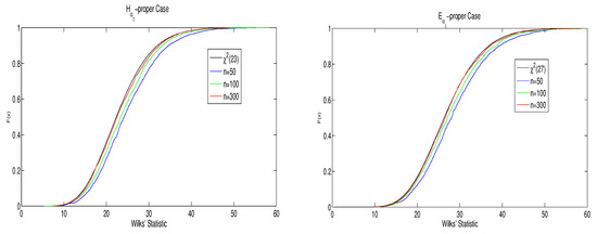
Figure 1. Wilks’ statistic for case 1 (left) and case 2 (right).

On the other hand, we assess the accuracy of the estimations of ${\alpha }_0$ depending on the sample size n. The maximization process in (9) can be achieved using the optimization toolbox in Matlab (The Nelder–Mead search algorithm is used). Table 2 and Table 3 depict the 95% confidence intervals for ${\alpha }_0$ obtained from 2000 simulated runs. As can be expected, the amplitudes of the confidence intervals become narrower as the sample size grows.

Table 2. The 95% confidence intervals for ${\alpha }_0$ in case 1.

n	50	100	300	500
C.I.	[1.506, 2.615]	[1.642, 2.433]	[1.788, 2.236]	[1.835, 2.190]

Table 3. The 95% confidence intervals for ${\alpha }_0$ in case 2.

n	50	100	300	500
C.I.	[−2.650, −1.512]	[−2.443, −1.633]	[−2.233, −1.777]	[−2.181, −1.846]

4. Linear Estimation and Prediction

The objective of this section is to solve the linear estimation problem for proper GSQ random variables. Since it is not possible to define a norm in the set of GSQs then, we cannot apply the projection theorem to obtain the optimum linear estimator. So, we first need to define a suitable metric and thus, we prove the existence and the uniqueness of the projection.

Given the random variables $x,y\in \mathbb{S}$, we define the product

$${⟨x,y⟩}_{\alpha }=E\left[x{y}_{\alpha }\right]={\mathsf{\Gamma }}_{xy}^3\left(\alpha \right)$$

where ${\mathsf{\Gamma }}_{xy}^3\left(\alpha \right)$ is the scalar version of ${\mathsf{\Gamma }}_{\mathbf{x}\mathbf{y}}^3\left(\alpha \right)$ given in (2).

For any random variables $x,y,u,v\in \mathbb{S}$ and deterministic coefficients $\lambda ,\beta \in \mathbb{S}$, $\gamma ,\delta \in \mathbb{R}$, it follows that

• ${⟨\lambda x+\beta y,\gamma u+\delta v⟩}_{\alpha }=\lambda \gamma {⟨x,u⟩}_{\alpha }+\lambda \delta {⟨x,v⟩}_{\alpha }+\beta \gamma {⟨y,u⟩}_{\alpha }+\beta \delta {⟨y,v⟩}_{\alpha }$.
• ${⟨x,x⟩}_{\alpha }=0\iff x=0$.

Thus, we can define a distance as

$$d_{\alpha }(x,y)={\parallel x-y\parallel }_{\alpha }$$

(11)

where ${\parallel x\parallel }_{\alpha }^2=\mathcal{R}\left\{{\mathsf{\Gamma }}_x^3\left(\alpha \right)\right\}$.

Consider the set of random vectors ${\mathcal{C}}_{\alpha }=\{{\mathbf{x}}_1,\dots ,{\mathbf{x}}_m\}$, with ${\mathbf{x}}_i\in {\mathbb{S}}^p$, $i=1,\dots ,m$, and denote by ${\mathcal{G}}_{{\mathcal{C}}_{\alpha }}$ the linear span of ${\mathcal{C}}_{\alpha }$, i.e., the set of all finite linear combinations of elements of ${\mathcal{C}}_{\alpha }$. The issue of existence and uniqueness of the projection of a given random variable $y\in \mathbb{S}$ onto the set ${\mathcal{G}}_{{\mathcal{C}}_{\alpha }}$ is now briefly investigated. This projection is denoted by ${\widehat{y}}_{\alpha }$.

In a metric space, neither the existence nor the uniqueness of ${\widehat{y}}_{\alpha }$ is assured; however, following a reasoning similar to [24], the existence and uniqueness of ${\widehat{y}}_{\alpha }$ can be proved. Further, ${\widehat{y}}_{\alpha }$ is the projection of y onto the set ${\mathcal{G}}_{{\mathcal{C}}_{\alpha }}$ if, and only if, ${⟨y-{\widehat{y}}_{\alpha },x⟩}_{\alpha }=0$, $\forall x\in {\mathcal{G}}_{{\mathcal{C}}_{\alpha }}$. As a consequence, if $\{{\vartheta }_1,\dots ,{\vartheta }_r\}$ is a basis of ${\mathcal{G}}_{{\mathcal{C}}_{\alpha }}$ then,

$${\widehat{y}}_{\alpha }=\sum _{i=1}^r{h}_i{\vartheta }_i$$

(12)

where the deterministic coefficients $h_i\in \mathbb{S}$ are obtained from the system

$${⟨y,{\vartheta }_j⟩}_{\alpha }=\sum _{i=1}^r{h}_i{⟨{\vartheta }_i,{\vartheta }_j⟩}_{\alpha }, j=1,\dots ,r$$

Now, we are prepared to introduce the notion of linear estimator in the GSQ domain.

Definition 2.

The projection of y onto the set ${\mathcal{G}}_{{\mathcal{C}}_{\alpha }}$, ${\widehat{y}}_{\alpha }$, is called the ${\mathbb{S}}_{\alpha }$ estimator of y respect to ${\mathcal{C}}_{\alpha }$ and, from now on, it is denoted by ${\widehat{y}}_{\alpha }^S$. If the information set is formed by augmented vectors defined in (5), i.e., if we consider ${\overline{\mathcal{C}}}_{\alpha }=\{{\overline{\mathbf{x}}}_1,\dots ,{\overline{\mathbf{x}}}_m\}$ with ${\overline{\mathbf{x}}}_i\in {\mathbb{S}}^{4p}$, $i=1,\dots ,m$, then, the projection of y onto the set ${\mathcal{G}}_{{\overline{\mathcal{C}}}_{\alpha }}$ is called SWL estimator of y respect to ${\mathcal{C}}_{\alpha }$ and it is denoted by ${\widehat{y}}_{\alpha }^{SWL}$.

These concepts are easily extended to the vectorial case. For example, the ${\mathbb{S}}_{\alpha }$ estimator of the random vector $\mathbf{y}\in {\mathbb{S}}^q$ respect to ${\mathcal{C}}_{\alpha }$ is ${\hat{\mathbf{y}}}_{\alpha }^{\mathtt{S}}=[{\widehat{y}}_{1\alpha }^{\mathtt{S}},\dots ,{\widehat{y}}_{q\alpha }^{\mathtt{S}}]$, where ${\widehat{y}}_{j\alpha }^{\mathtt{S}}$ is the projection of the component jth of $\mathbf{y}$ onto the set ${\mathcal{G}}_{{\mathcal{C}}_{\alpha }}$.

Theorem 2.

Consider a random variable $y\in \mathbb{S}$ and the set of random vectors ${\mathcal{C}}_{\alpha }=\{{\mathbf{x}}_1,\dots ,{\mathbf{x}}_m\}$, with ${\mathbf{x}}_i\in {\mathbb{S}}^p$, $i=1,\dots ,m$. Then,

• The SWL estimator of y respect to ${\mathcal{C}}_{\alpha }$ is obtained as

  $${\widehat{y}}_{\alpha }^{SWL}=\sum _{i=1}^m({\mathbf{h}}_{1i}^{\mathtt{T}}\left(\alpha \right){\mathbf{x}}_i+{\mathbf{h}}_{2i}^{\mathtt{T}}\left(\alpha \right){\mathbf{x}}_i^{\mathrm{i}}+{\mathbf{h}}_{3i}^{\mathtt{T}}\left(\alpha \right){\mathbf{x}}_i^{\mathrm{j}}+{\mathbf{h}}_{4i}^{\mathtt{T}}\left(\alpha \right){\mathbf{x}}_i^{\mathrm{k}})$$

  where the deterministic vectors ${\mathbf{h}}_{ji}\left(\alpha \right)\in {\mathbb{S}}^p$ are computed through the equation

  $$\begin{array}{c}[{\mathbf{h}}_{11}^{\mathtt{T}}\left(\alpha \right),\dots ,{\mathbf{h}}_{1m}^{\mathtt{T}}\left(\alpha \right),{\mathbf{h}}_{21}^{\mathtt{T}}\left(\alpha \right),\dots ,{\mathbf{h}}_{2m}^{\mathtt{T}}\left(\alpha \right),\\ {\mathbf{h}}_{31}^{\mathtt{T}}\left(\alpha \right),\dots ,{\mathbf{h}}_{3m}^{\mathtt{T}}\left(\alpha \right),{\mathbf{h}}_{41}^{\mathtt{T}}\left(\alpha \right),\dots ,{\mathbf{h}}_{4m}^{\mathtt{T}}\left(\alpha \right)]={\mathsf{\Gamma }}_{y\overline{\mathbf{z}}}^3\left(\alpha \right){\mathsf{\Gamma }}_{\overline{\mathbf{z}}}^{3^{-1}}\left(\alpha \right)\end{array}$$

  (13)

  with $\overline{\mathbf{z}}={[{\mathbf{x}}_1^{\mathtt{T}},\dots ,{\mathbf{x}}_m^{\mathtt{T}},{\mathbf{x}}_1^{\mathrm{i}\mathtt{T}},\dots ,{\mathbf{x}}_m^{\mathrm{i}\mathtt{T}},{\mathbf{x}}_1^{\mathrm{j}\mathtt{T}},\cdots ,{\mathbf{x}}_m^{\mathrm{j}\mathtt{T}},{\mathbf{x}}_1^{\mathrm{k}\mathtt{T}},\dots ,{\mathbf{x}}_m^{\mathrm{k}\mathtt{T}}]}^{\mathtt{T}}$.
  Moreover, this estimator and its associated error are independent of the value of α, i.e., ${\widehat{y}}^{SWL}={\widehat{y}}_{\alpha }^{SWL}$ and ${ϵ}^{SWL}={ϵ}_{\alpha }^{SWL}$, $\forall \alpha \ne 0$, where ${ϵ}_{\alpha }^{SWL}={\parallel y-{\widehat{y}}_{\alpha }^{SWL}\parallel }_{\alpha }^2$.
• The ${\mathbb{S}}_{\alpha }$ estimator of y respect to ${\mathcal{C}}_{\alpha }$ is calculated as

  $${\widehat{y}}_{\alpha }^S=\sum _{i=1}^m{\mathbf{g}}_i^{\mathtt{T}}\left(\alpha \right){\mathbf{x}}_i$$

  where the deterministic vectors ${\mathbf{g}}_i\left(\alpha \right)\in {\mathbb{S}}^p$ are computed through the equation

  $$[{\mathbf{g}}_1^{\mathtt{T}}\left(\alpha \right),\dots ,{\mathbf{g}}_m^{\mathtt{T}}\left(\alpha \right)]={\mathsf{\Gamma }}_{y\mathbf{z}}^3\left(\alpha \right){\mathsf{\Gamma }}_{\mathbf{z}}^{3^{-1}}\left(\alpha \right)$$

  (14)

  with

  $$\mathbf{z}={[{\mathbf{x}}_1^{\mathtt{T}},\dots ,{\mathbf{x}}_m^{\mathtt{T}}]}^{\mathtt{T}}$$

  (15)
• ${ϵ}^{SWL}\le {ϵ}_{\alpha }^{\mathtt{S}}={\parallel y-{\widehat{y}}_{\alpha }^{\mathtt{S}}\parallel }_{\alpha }^2,\forall \alpha \ne 0$.
• If ${\mathbf{x}}_1,\dots ,{\mathbf{x}}_m$ are jointly $H_{{\alpha }_0}$-proper (respectively, $E_{{\alpha }_0}$-proper) and y is cross $H_{{\alpha }_0}$-proper (respectively, $E_{{\alpha }_0}$-proper) with each element of $\{{\mathbf{x}}_1,\dots ,{\mathbf{x}}_m\}$ then, ${\widehat{y}}^{SWL}={\widehat{y}}_{{\alpha }_0}^S$.

Remark 2.

Theorem 2 shows that whatever hypercomplex algebra you choose provides the same SWL estimator. Likewise, the computational burden of the SWL estimator can be notably reduced whenever hyperbolic or elliptic conditions of properness are fulfilled (compare (13) with (14)). Effectively, while the computational complexity of SWL estimators is of order $\mathcal{O}\left(64p^3{m}^3\right)$, this is of order $\mathcal{O}\left(p^3{m}^3\right)$ under hyperbolic or elliptic properness. More importantly, this reduction in computational complexity cannot be achieved in the real numbers domain.

Now, we are concerned with the prediction problem for random signals. Consider a random signal vector $\mathbf{x}\left(t\right)\in {\mathbb{S}}^p$. Our aim is to obtain the ${\mathbb{S}}_{\alpha }$ one-stage predictor of $\mathbf{x}(t+1)$ from the information contained in the set ${\mathcal{C}}_{\alpha }^t=\{\mathbf{x}\left(1\right),\dots ,\mathbf{x}\left(t\right)\}$, denoted by ${\hat{\mathbf{x}}}_{\alpha }^{\mathtt{S}}(t+1|t)$. Analogously, the SWL one-stage predictor is denoted by ${\hat{\mathbf{x}}}^{\mathtt{SWL}}(t+1|t)$.

Note that a similar result to Theorem 2 can be stated for random signals, but we do not include it here for the sake of brevity. It should be remarked, however, that a computational problem remains still unsolved. Although the estimation problem is indeed simplified due to the reduction in dimension implied by the properness conditions, we have to cope with the inverse in (14) as the number of observations t grows. The following result overcomes this problem for proper signals.

Theorem 3

(The innovations algorithm). Consider a $H_{{\alpha }_0}$-proper (respectively, $E_{{\alpha }_0}$-proper) random signal vector $\mathbf{x}\left(t\right)\in {\mathbb{S}}^p$. If ${\mathsf{\Gamma }}_{\mathbf{x}}^{\nu }({\alpha }_0,t,s)$ is nonsingular for $\nu =1,2$ then, ${\hat{\mathbf{x}}}^{SWL}(t+1|t)={\hat{\mathbf{x}}}_{{\alpha }_0}^S(t+1|t)$ and can be recursively obtained in the following way:

$${\hat{\mathbf{x}}}_{{\alpha }_0}^S(t+1|t)=\sum _{i=1}^t\mathsf{\Lambda }(t,i)(\mathbf{x}(t+1-i)-{\hat{\mathbf{x}}}_{{\alpha }_0}^S(t+1-i|t-i)) t\ge 1$$

(16)

with ${\hat{\mathbf{x}}}_{{\alpha }_0}^S\left(1\right|0)={\mathbf{0}}_{p\times 1}$ and where

$$\mathsf{\Lambda }(t,t-k)=({\mathsf{\Gamma }}_{\mathbf{x}}^{\nu }({\alpha }_0,t+1,k+1)-\sum _{i=0}^{k-1}\mathsf{\Lambda }(t,t-i)\mathsf{\Pi }\left(i\right){\mathsf{\Lambda }}^{H_{3-2\nu }}(k,k-i)){\mathsf{\Pi }}^{-1}\left(k\right)$$

(17)

for $k=1,\dots ,t-1$, with $\mathsf{\Lambda }(t,t)={\mathsf{\Gamma }}_{\mathbf{x}}^{\nu }({\alpha }_0,t+1,1){\mathsf{\Pi }}^{-1}\left(0\right)$ and

$$\mathsf{\Pi }\left(t\right)={\mathsf{\Gamma }}_{\mathbf{x}}^{\nu }({\alpha }_0,t+1,t+1)-\sum _{i=0}^{t-1}\mathsf{\Lambda }(t,t-i)\mathsf{\Pi }\left(i\right){\mathsf{\Lambda }}^{H_{3-2\nu }}(t,t-i)$$

(18)

with the initial condition $\mathsf{\Pi }\left(0\right)={\mathsf{\Gamma }}_{\mathbf{x}}^{\nu }({\alpha }_0,1,1)$. Moreover, the error associated to the component $x_j(t+1)$ is given by

$${ϵ}_j^{SWL}(t+1|t)=\frac{2|{\alpha }_0|+2}{4|{\alpha }_0|}\mathcal{R}\left\{{\mathsf{\Pi }}_{jj}\left(t\right)\right\}$$

(19)

5. Proper ARMA Models

This section constitutes the core of the paper. Starting from the definition of proper ARMA models in the GSQs domain we then solve the one-stage prediction problem.

5.1. ARMA Modeling

Next, we adapt the proper ARMA signal concept to the GSQs domain and extend the Yule–Walker equations to this kind of signals. To do so, we first extend the concept of stationarity to the GSQs domain in the proper signal scenario.

Definition 3.

A $H_{{\alpha }_0}$-proper random signal vector $\mathbf{x}\left(t\right)\in {\mathbb{S}}^p$ is said to be stationary if ${\mathsf{\Gamma }}_{\mathbf{x}}^1({\alpha }_0,t+h,t)={\mathsf{\Gamma }}_{\mathbf{x}}^1({\alpha }_0,s+h,s)$, $\forall t,s,h\in \mathbb{Z}$, i.e., ${\mathsf{\Gamma }}_{\mathbf{x}}^1$ only depends on the lag h for a given ${\alpha }_0$. In this case, we denote ${\mathsf{\Gamma }}_{\mathbf{x}}^1({\alpha }_0,h)={\mathsf{\Gamma }}_{\mathbf{x}}^1({\alpha }_0,t+h,t)$. The concept of a $E_{{\alpha }_0}$-proper stationary signal is defined analogously by replacing ${\mathsf{\Gamma }}_{\mathbf{x}}^1$ by ${\mathsf{\Gamma }}_{\mathbf{x}}^2$.

Definition 4.

A random signal vector $\mathbf{x}\left(t\right)\in {\mathbb{S}}^p$ is said to be a $H_{{\alpha }_0}$-proper ARMA signal of orders p and q (ARMA($p,q$)) if it is $H_{{\alpha }_0}$-proper, stationary, and can be modeled by the following system:

$$\mathbf{x}\left(t\right)=\sum _{i=1}^p\mathbf{F}\left(i\right)\mathbf{x}(t-i)+\sum _{i=0}^q\mathbf{G}\left(i\right)\mathbf{v}(t-i)$$

(20)

where $\mathbf{G}\left(0\right)={\mathbf{I}}_p$, $\mathbf{F}\left(i\right),\mathbf{G}\left(i\right)\in {\mathbb{S}}^{p\times p}$ are deterministic matrices and $\mathbf{v}\left(t\right)$ is a $H_{{\alpha }_0}$-proper white noise verifying

$${\mathsf{\Gamma }}_{\mathbf{v}}^1({\alpha }_0,t,s)=\mathsf{\Omega }{\delta }_{ts}$$

(21)

with $\mathsf{\Omega }\in {\mathbb{S}}^{p\times p}$ a deterministic matrix.

The concept of a $E_{{\alpha }_0}$-proper ARMA($p,q$) signal is defined analogously by replacing $H_{{\alpha }_0}$-proper by $E_{{\alpha }_0}$-proper, and ${\mathsf{\Gamma }}_{\mathbf{v}}^1$ by ${\mathsf{\Gamma }}_{\mathbf{v}}^2$ in (21).

The following result extends the Yule–Walker equations to the case of proper ARMA signals.

Proposition 2.

Let $\mathbf{x}\left(t\right)\in {\mathbb{S}}^p$ be a $H_{{\alpha }_0}$-proper (or $E_{{\alpha }_0}$-proper) ARMA($p,q$) signal. Consider the matrix-valued polynomial $\mathfrak{F}\left(z\right)={\mathbf{I}}_{4p}-{\sum }_{i=1}^p\overline{\mathbf{F}}\left(i\right)z^i$ with $\overline{\mathbf{F}}\left(i\right)=diag(\mathbf{F}\left(i\right),{\mathbf{F}}^{\mathrm{i}}\left(i\right),{\mathbf{F}}^{\mathrm{j}}\left(i\right),{\mathbf{F}}^{\mathrm{k}}\left(i\right))$, $i=1,\dots ,p$. If $det{\left(\mathfrak{F}\left(z\right)\right)}_{{\alpha }_0}\ne 0$, $\forall z\in \mathbb{C}$ such that $\left|z\right|\le 1$ then, ${\mathsf{\Gamma }}_{\mathbf{x}}^{\nu }({\alpha }_0,h)$, $\nu =1,2$, obeys the equation

$${\mathsf{\Gamma }}_{\mathbf{x}}^{\nu }({\alpha }_0,h)-\sum _{i=1}^p\mathbf{F}\left(i\right){\mathsf{\Gamma }}_{\mathbf{x}}^{\nu }({\alpha }_0,h-i)=\sum _{h\le i\le q}\mathbf{G}\left(i\right)\mathsf{\Omega }{\mathbf{L}}^{H_{3-2\nu }}(i-h), h\ge 0$$

(22)

where the matrices $\mathbf{L}\left(t\right)$ are determined by

$$\begin{array}{cc}\hfill \mathbf{L}\left(0\right)& ={\mathbf{I}}_p, \mathbf{L}\left(t\right)={\mathbf{0}}_{p\times p}, t<0\hfill \\ \hfill \mathbf{L}\left(t\right)& =\sum _{i=1}^t\mathbf{F}\left(i\right)\mathbf{L}(t-i)+\mathbf{G}\left(t\right), t\ge 1\hfill \end{array}$$

with $\mathbf{F}\left(t\right)={\mathbf{0}}_{p\times p}$, $t>p$ and $\mathbf{G}\left(t\right)={\mathbf{0}}_{p\times p}$, $t>q$.

5.2. One-Stage Prediction

We aim to improve the recursive algorithm for ${\widehat{\mathbf{x}}}_{{\alpha }_0}^{\mathtt{S}}(t+1|t)$ given in Theorem 3 by making use of the particular structure of proper ARMA($p,q$) models.

Theorem 4.

Let $\mathbf{x}\left(t\right)\in {\mathbb{S}}^p$ be a $H_{{\alpha }_0}$-proper (or $E_{{\alpha }_0}$-proper) ARMA($p,q$) signal. If $det{\left(\mathfrak{F}\left(z\right)\right)}_{{\alpha }_0}\ne 0$, $\forall z\in \mathbb{C}$ such that $\left|z\right|\le 1$ then, ${\widehat{\mathbf{x}}}^{SWL}(t+1|t)={\widehat{\mathbf{x}}}_{{\alpha }_0}^S(t+1|t)$ and this predictor can be calculated through the following recursive procedure:

$${\widehat{\mathbf{x}}}_{{\alpha }_0}^S(t+1|t)=\{\begin{array}{cc}{\displaystyle \sum _{i=1}^t\mathsf{\Lambda }(t,i)(\mathbf{x}(t+1-i)-{\widehat{\mathbf{x}}}_{{\alpha }_0}^S(t+1-i|t-i)),}\hfill & 1\le t<m\hfill \\ {\displaystyle \sum _{i=1}^p\mathbf{F}\left(i\right)\mathbf{x}(t+1-i)+\sum _{i=1}^q\mathsf{\Lambda }(t,i)(\mathbf{x}(t+1-i)-{\widehat{\mathbf{x}}}_{{\alpha }_0}^S(t+1-i|t-i)),}\hfill & t\ge m\hfill \end{array}$$

(23)

with ${\widehat{\mathbf{x}}}_{{\alpha }_0}^S\left(1\right|0)={\mathbf{0}}_{p\times 1}$, $m=max(p,q)$ and the matrices $\mathsf{\Lambda }(t,i)$ are calculated by replacing ${\mathsf{\Gamma }}_{\mathbf{x}}^{\nu }$ in (17) and (18) by the following function:

$${{\rm Y}}^{\nu }(t,s)=\{\begin{array}{cc}{\mathsf{\Gamma }}_{\mathbf{x}}^{\nu }({\alpha }_0,t-s),\hfill & 1\le t\le s\le m\hfill \\ {\displaystyle {\mathsf{\Gamma }}_{\mathbf{x}}^{\nu }({\alpha }_0,t-s)-\sum _{i=1}^p{\mathsf{\Gamma }}_{\mathbf{x}}^{\nu }({\alpha }_0,t+i-s){\mathbf{F}}^{H_{3-2\nu }}\left(i\right),}\hfill & 1\le t\le m\le s\le 2m\hfill \\ {\mathbf{0}}_{p\times p},\hfill & 1\le t\le m,s>2m\hfill \\ {\displaystyle \sum _{i=0}^q\mathbf{G}\left(i\right)\mathsf{\Omega }{\mathbf{G}}^{H_{3-2\nu }}(i+s-t), }\hfill & m<t\le s\le t+q\hfill \\ {\mathbf{0}}_{p\times p},\hfill & m<t,t+q<s\hfill \\ {{\rm Y}}^{\nu H_{3-2\nu }}(s,t),\hfill & s<t\hfill \end{array}$$

(24)

with $\mathbf{G}\left(i\right)={\mathbf{0}}_{p\times p}$ for $i>q$, Ω given in (21), and ${\mathsf{\Gamma }}_{\mathbf{x}}^{\nu }({\alpha }_0,t-s)$ obeys (22). Moreover, the error associated to (23) coincides with (19).

Remark 3.

The advantage of working with this algorithm is that ${{\rm Y}}^{\nu }(t,s)={\mathbf{0}}_{p\times p}$ for $|s-t|>q$ and thus, unlike the innovations algorithm given in Theorem 3, only $\mathsf{\Lambda }(t,i)$, for $i=1,\dots ,q$, have to be computed in each recursion.

Corollary 1.

For an ARMA($1,1$) signal it follows that

$${{\rm Y}}^{\nu }(t,s)=\{\begin{array}{cc}{\mathsf{\Gamma }}_{\mathbf{x}}^{\nu }({\alpha }_0,0),\hfill & t=s=1\hfill \\ \mathsf{\Omega }{\mathbf{G}}^{H_{3-2\nu }}\left(1\right),\hfill & 1\le t,s=t+1\hfill \\ \mathsf{\Omega }+\mathbf{G}\left(1\right)\mathsf{\Omega }{\mathbf{G}}^{H_{3-2\nu }}\left(1\right),\hfill & 1<t=s\hfill \\ {\mathbf{0}}_{p\times p},\hfill & 1\le t,t+1<s\hfill \\ {{\rm Y}}^{\nu H_{3-2\nu }}(s,t),\hfill & s<t\hfill \end{array}, \nu =1,2$$

and the one-stage predictor is computed through

$${\widehat{\mathbf{x}}}_{{\alpha }_0}^S(t+1|t)=\mathbf{F}\left(1\right)\mathbf{x}\left(t\right)+\mathsf{\Lambda }(t,1)(\mathbf{x}\left(t\right)-{\widehat{\mathbf{x}}}_{{\alpha }_0}^S\left(t\right|t-1)), t\ge 1$$

(25)

where

$$\begin{array}{cc}\hfill \mathsf{\Lambda }(t,1)& =\mathbf{G}\left(1\right)\mathsf{\Omega }{\mathsf{\Pi }}^{-1}(t-1)\hfill \\ \hfill \mathsf{\Pi }\left(t\right)& =\mathsf{\Omega }+\mathbf{G}\left(1\right)\mathsf{\Omega }{\mathbf{G}}^{{\mathtt{H}}_{3-2\nu }}\left(1\right)-\mathsf{\Lambda }(t,1)\mathsf{\Pi }(t-1){\mathsf{\Lambda }}^{{\mathtt{H}}_{3-2\nu }}(t,1)\hfill \end{array}$$

(26)

and $\mathsf{\Pi }\left(0\right)={\mathsf{\Gamma }}_{\mathbf{x}}^{\nu }({\alpha }_0,0)$ is computed solving the following system of matrix equations:

$$\begin{array}{cc}\hfill {\mathsf{\Gamma }}_{\mathbf{x}}^{\nu }({\alpha }_0,0)-\mathbf{F}\left(1\right){\mathsf{\Gamma }}_{\mathbf{x}}^{\nu H_{3-2\nu }}({\alpha }_0,-1)& =\mathsf{\Omega }+\mathbf{G}\left(1\right)\mathsf{\Omega }({\mathbf{F}}^{H_{3-2\nu }}\left(1\right)+{\mathbf{G}}^{{\mathtt{H}}_{3-2\nu }}\left(1\right))\hfill \\ \hfill {\mathsf{\Gamma }}_{\mathbf{x}}^{\nu }({\alpha }_0,1)-\mathbf{F}\left(1\right){\mathsf{\Gamma }}_{\mathbf{x}}^{\nu }({\alpha }_0,0)& =\mathbf{G}\left(1\right)\mathsf{\Omega }\hfill \end{array}$$

To conclude, a steady-state performance analysis for the one-stage predictor (23) and its associated error is fulfilled.

Corollary 2.

Under conditions of Theorem 4, if $\mathfrak{G}\left(z\right)$ given in (A4) satisfies $det{\left(\mathfrak{G}\left(z\right)\right)}_{{\alpha }_0}\ne 0$, $\forall z\in \mathbb{C}$ such that $\left|z\right|\le 1$, then,

$$\mathsf{\Lambda }(t,i)\stackrel{t\uparrow \infty }{\to }\mathbf{G}\left(i\right), {ϵ}_j^{SWL}(t+1|t)\stackrel{t\uparrow \infty }{\to }{ϵ}_j$$

(27)

with

$${ϵ}_j=\frac{2|{\alpha }_0|+2}{4|{\alpha }_0|}\mathcal{R}\left\{{\Omega }_{jj}\right\}$$

(28)

being ${\mathsf{\Omega }}_{jj}$ the jth diagonal entry of Ω given in (21).

5.3. Example

By way of illustration, we consider a proper ARMA(1,1) model. With this model, we first carry out a performance comparative analysis between the ${\mathbb{S}}_{{\alpha }_0}$ one-stage predictor (25), and its counterpart in the HQ domain, ${\widehat{x}}_{{\alpha }_0}^{QSL}(t+1|t)$. Our aim is to show the superiority in terms of performance of the proposed approach respect to the usual HQ methodology under different initial conditions. Finally, a steady-state performance analysis is carried out.

Let the ARMA(1,1) system be

$$x\left(t\right)=fx(t-1)+v\left(t\right)+gv(t-1)$$

with $f=0.3-0.05\mathrm{j}+0.1\mathrm{k}$, $g=0.1+0.2\mathrm{j}+0.4\mathrm{k}$ and $v\left(t\right)$ a white noise whose real vector (3) verifies ${\mathsf{\Gamma }}_{{\mathbf{v}}_r}(t,s)=\Omega {\delta }_{ts}$ where $\Omega$ is the matrix given in (10).

Two scenarios are contemplated: in the first one, we consider that $\lambda =-0.7$ and $\mu =0.8$ in $\Omega$, and three different hyperbolic quaternion algebras are studied (${\alpha }_0=1,2,3$). In the second one, we set the value of the parameters $\lambda$ and $\mu$ to be both 0 and three elliptic quaternion algebras are analyzed (${\alpha }_0=-1,-2,-3$). These scenarios present an interesting characteristic: from Proposition 1, $x\left(t\right)$ is either $H_{{\alpha }_0}$-proper (in scenario 1) or $E_{{\alpha }_0}$-proper (in scenario 2); however, the degree of improperness of $x\left(t\right)$ in the HQ system increases as $|{\alpha }_0|$ grows.

Note that the conditions of Proposition 2 and Corollary 2 are fulfilled and hence, ${\widehat{x}}_{{\alpha }_0}^{\mathtt{S}}(t+1|t)$ can be obtained through the recursions (25) and (26) and the steady-state results in (27) hold.

The errors associated to ${\widehat{x}}_{{\alpha }_0}^{\mathtt{S}}(t+1|t)$ and ${\widehat{x}}_{{\alpha }_0}^{\mathtt{QSL}}(t+1|t)$ depend on the value ${\alpha }_0$ and thus, they are denoted by ${ϵ}_{{\alpha }_0}^{\mathtt{SWL}}(t+1|t)$ and ${ϵ}_{{\alpha }_0}^{\mathtt{QSL}}(t+1|t)$, respectively. To assess the performance of both approaches, the following measure is computed:

$$D{P}_{{\alpha }_0}\left(t\right)={ϵ}_{{\alpha }_0}^{\mathtt{QSL}}(t+1|t)-{ϵ}_{{\alpha }_0}^{\mathtt{SWL}}(t+1|t)$$

(29)

Figure 2 depicts the measure $D{P}_{{\alpha }_0}\left(t\right)$ in (29), for $t=1,\dots ,100$, in the above two scenarios. As can be seen, the ${\mathbb{S}}_{{\alpha }_0}$ one-stage predictor outperforms the HQ one-stage predictor in both scenarios. Furthermore, the measure becomes greater as $|{\alpha }_0|$ grows, i.e., as the degree of HQ improperness grows; being $D{P}_{{\alpha }_0}\left(t\right)$ slightly greater for the $E_{{\alpha }_0}$-proper case.

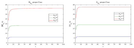
Figure 2. $D{P}_{{\alpha }_0}\left(t\right)$ in scenarios 1 (left) and 2 (right).

Now, we analyze the steady-state performance of both the estimate (25) and its error. The errors (28) computed for different values of ${\alpha }_0$ appear in Table 4. Further, Figure 3 shows as ${ϵ}_{{\alpha }_0}^{\mathtt{SWL}}(t+1|t)$ converges toward their respective steady-state errors when t grows. These plots indicate that the convergence is rapid.

Table 4. Steady-state errors of the one-stage predictor for the different values of ${\alpha }_0$.

$|{\mathit{\alpha }}_0|$	1	2	3
$ϵ$	24	36	48

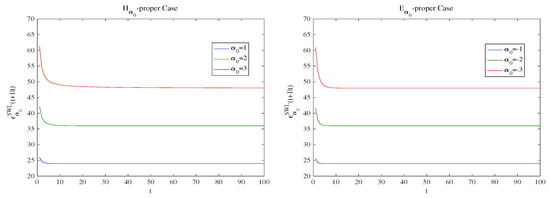
Figure 3. ${ϵ}_{{\alpha }_0}^{\mathtt{SWL}}(t+1|t)$ for ${\alpha }_0=-3,-2,-1,1,2,3$.

Finally, Figure 4 displays the convergence performance of the components of $\Lambda (t,1)={\Lambda }_1(t,1)+{\Lambda }_2(t,1)\mathrm{i}+{\Lambda }_3(t,1)\mathrm{j}+{\Lambda }_4(t,1)\mathrm{k}$ given in (26). As could be expected from (27), we also obtain here a rapid convergence toward the target values and, in general, this convergence is slightly slower as $|{\alpha }_0|$ grows as well as in the $H_{{\alpha }_0}$-proper case.

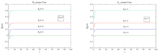
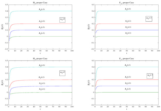
Figure 4. Values of the components ${\Lambda }_i(t,1)$, $i=1,\dots ,4$, for ${\alpha }_0=-3,-2,-1,1,2,3$.

6. Discussion

Recent investigations have shown that HQs are not always the best choice for processing 4D hypercomplex signals. These results suggest distinct strategies depending on whether properness conditions are complied with. As the main characteristic, they offer a significant computational saving in relation to the real-valued processing. Unlike earlier research, the approach described in this paper has the additional advantage of the flexibility in the choice of the hypercomplex algebra. In our opinion, this research topic opens a broad range of possibilities for studying new applications in signal processing. This paper precisely proposes the time series analysis as a possible field of application of the proper GSQ signal processing. Other potential areas include dynamic linear models, filtering and smoothing, signal detection, etc.

References

- Pollock, D.S.G. A Handbook of Time-Series Analysis, Signal Processing and Dynamics; Academic Press: San Diego, CA, USA, 1999. [Google Scholar]
- Manolakis, D.; Bosowski, N.; Ingle, V.K. Count time-series analysis: A signal processing perspective. IEEE Signal Process. Mag. 2019, 36, 64–81. [Google Scholar] [CrossRef]
- Brockwell, P.J.; Davis, R.A. Time Series: Theory and Methods, 2nd ed.; Springer: New York, NY, USA, 1991. [Google Scholar]
- Kuipers, J.B. Quaternions and Rotation Sequences: A Primer with Applications to Orbits, Aerospace and Virtual Reality; Princeton University Press: Princeton, NJ, USA, 2002. [Google Scholar]
- Hanson, A.J. Visualizing Quaternions; The Morgan Kaufmann Series in Interactive 3D Technology; Elsevier: Amsterdam, The Netherlands, 2005. [Google Scholar]
- Catoni, F.; Boccaletti, D.; Cannata, R.; Catoni, V.; Nichelatti, E.; Zampetti, P. The Mathematics of Minkowski Space-Time: With an Introduction to Commutative Hypercomplex Numbers; Birkhaüser Verlag: Basel, Switzerland, 2008. [Google Scholar]
- Ginzberg, P.; Walden, A.T. Quaternion VAR modelling and estimation. IEEE Trans. Signal Process. 2013, 61, 154–158. [Google Scholar] [CrossRef] [Green Version]
- Tobar, F.; Mandic, D.P. Quaternion reproducing kernel Hilbert spaces: Existence and uniqueness conditions. IEEE Trans. Inform. Theory 2014, 60, 5736–5749. [Google Scholar] [CrossRef]
- Schütte, H.D.; Wenzel, J. Hypercomplex numbers in digital signal processing. In Proceedings of the International Symposium on Circuits and Systems, New Orleans, LA, USA, 1–3 May 1990; pp. 1557–1560. Available online: https://ieeexplore.ieee.org/document/112431 (accessed on 15 February 2022).
- Pei, S.H.; Chang, J.H.; Ding, J.J. Commutative reduced biquaternions and their Fourier transform for signal and image processing applications. IEEE Trans. Signal Process. 2004, 52, 2012–2031. [Google Scholar] [CrossRef]
- Labunets, V. Clifford algebras as unified language for image processing and pattern recognition. In Computational Noncommutative Algebra and Applications; NATO Science Series II: Mathematics, Physics and Chemistry; Byrnes, J., Ed.; Springer: Dordrecht, The Netherlands, 2004; Volume 136, pp. 197–225. [Google Scholar]
- Alfsmann, D. On families of 2N-dimensional hypercomplex algebras suitable for digital signal processing. In Proceedings of the 14th European Signal Processing Conference (EUSIPCO 2006), Florence, Italy, 4–8 September 2006; pp. 1–4. [Google Scholar]
- Alfsmann, D.; Göckler, H.G.; Sangwine, S.J.; Ell, T.A. Hypercomplex algebras in digital signal processing: Benefits and drawbacks. In Proceedings of the 15th European Signal Processing Conference, Poznan, Poland, 3–7 September 2007; pp. 1322–1326. [Google Scholar]
- Pei, S.H.; Chang, J.H.; Ding, J.J.; Chen, M.Y. Eigenvalues and singular value decompositions of reduced biquaternion matrices. IEEE Trans. Circuits Syst. I 2008, 525, 2673–2685. [Google Scholar]
- Guo, L.; Zhu, M.; Ge, X. Reduced biquaternion canonical transform, convolution and correlation. Signal Process. 2011, 91, 2147–2153. [Google Scholar] [CrossRef]
- Hahn, S.L.; Snopek, K.M. Complex and Hypercomplex Analytic Signals: Theory and Applications; Artech House: Norwood, MA, USA, 2016. [Google Scholar]
- Kamal, A.T.; El-Melegy, M.T. Color image processing using reduced biquaternions with applications to face recognition in a PCA framework. In Proceedings of the IEEE International Conference on Computer Vision Workshops, Venice, Italy, 22–29 October 2017; pp. 3039–3046. [Google Scholar]
- Esposito, A.; Faundez-Zanuy, M.; Morabito, F.C.; Pasero, E. Neural Advances in Processing Nonlinear Dynamic Signals; Springer: Cham, Switzerland, 2018. [Google Scholar]
- Kobayashi, M. Twin-multistate commutative quaternion Hopfield neural networks. Neurocomputing 2018, 320, 150–156. [Google Scholar] [CrossRef]
- Zanetti de Castro, F.; Eduardo Valle, M. A broad class of discrete-time hypercomplex-valued Hopfield neural networks. Neural Netw. 2020, 122, 54–67. [Google Scholar] [CrossRef] [Green Version]
- Takahashi, K. Comparison of high-dimensional neural networks using hypercomplex numbers in a robot manipulator control. Artif. Life Robot. 2021, 26, 367–377. [Google Scholar] [CrossRef]
- Ortolani, F.; Scarpiniti, M.; Comminiello, D.; Uncini, A. On the influence of microphone array geometry on the behavior of hypercomplex adaptive filters. In Proceedings of the 5th IEEE Microwaves, Radar and Remote Sensing Symposium (MRRS), Kiev, Ukraine, 29–31 August 2017; pp. 37–42. [Google Scholar]
- Ortolani, F.; Scarpiniti, M.; Comminiello, D.; Uncini, A. On 4-dimensional hypercomplex algebras in adaptive signal processing. In Neural Advances in Processing Nonlinear Dynamic Signals; Springer: Berlin, Germany, 2017; pp. 131–140. [Google Scholar]
- Navarro-Moreno, J.; Fernández-Alcalá, R.M.; López-Jiménez, J.D.; Ruiz-Molina, J.C. Tessarine signal processing under the T-properness condition. J. Frankl. Inst. 2020, 357, 10100–10126. [Google Scholar] [CrossRef]
- Navarro-Moreno, J.; Ruiz-Molina, J.C. Wide-sense Markov signals on the tessarine domain. A study under properness conditions. Signal Process. 2021, 183C, 108022. [Google Scholar] [CrossRef]
- Took, C.C.; Mandic, D.P. Augmented second-order statistics of quaternion random signals. Signal Process. 2011, 91, 214–224. [Google Scholar] [CrossRef] [Green Version]
- Navarro-Moreno, J.; Fernández-Alcalá, R.M.; Ruiz-Molina, J.C. Semi-widely simulation and estimation of continuous-time Cη-proper quaternion random signals. IEEE Trans. Signal Process. 2015, 63, 4999–5012. [Google Scholar] [CrossRef]
- Navarro-Moreno, J.; Ruiz-Molina, J.C. Semi-widely linear estimation of Cη-proper quaternion random signal vectors under Gaussian and stationary conditions. Signal Process. 2016, 119, 56–66. [Google Scholar] [CrossRef]
- Nitta, T.; Kobayashi, M.; Mandic, D.P. Hypercomplex widely linear estimation through the lens of underpinning geometry. IEEE Trans. Signal Process. 2019, 67, 3985–3994. [Google Scholar] [CrossRef]
- Grassucci, E.; Comminiello, D.; Uncini, A. An information-theoretic perspective on proper quaternion variational autoencoders. Entropy 2021, 23, 856. [Google Scholar] [CrossRef] [PubMed]
Publisher’s Note: MDPI stays neutral with regard to jurisdictional claims in published maps and institutional affiliations. |
© 2022 by the authors. Licensee MDPI, Basel, Switzerland. This article is an open access article distributed under the terms and conditions of the Creative Commons Attribution (CC BY) license (https://creativecommons.org/licenses/by/4.0/).