
Assessment of Machine Learning Methods for State-to-State Approach in Nonequilibrium Flow Simulations


Abstract
:1. Introduction
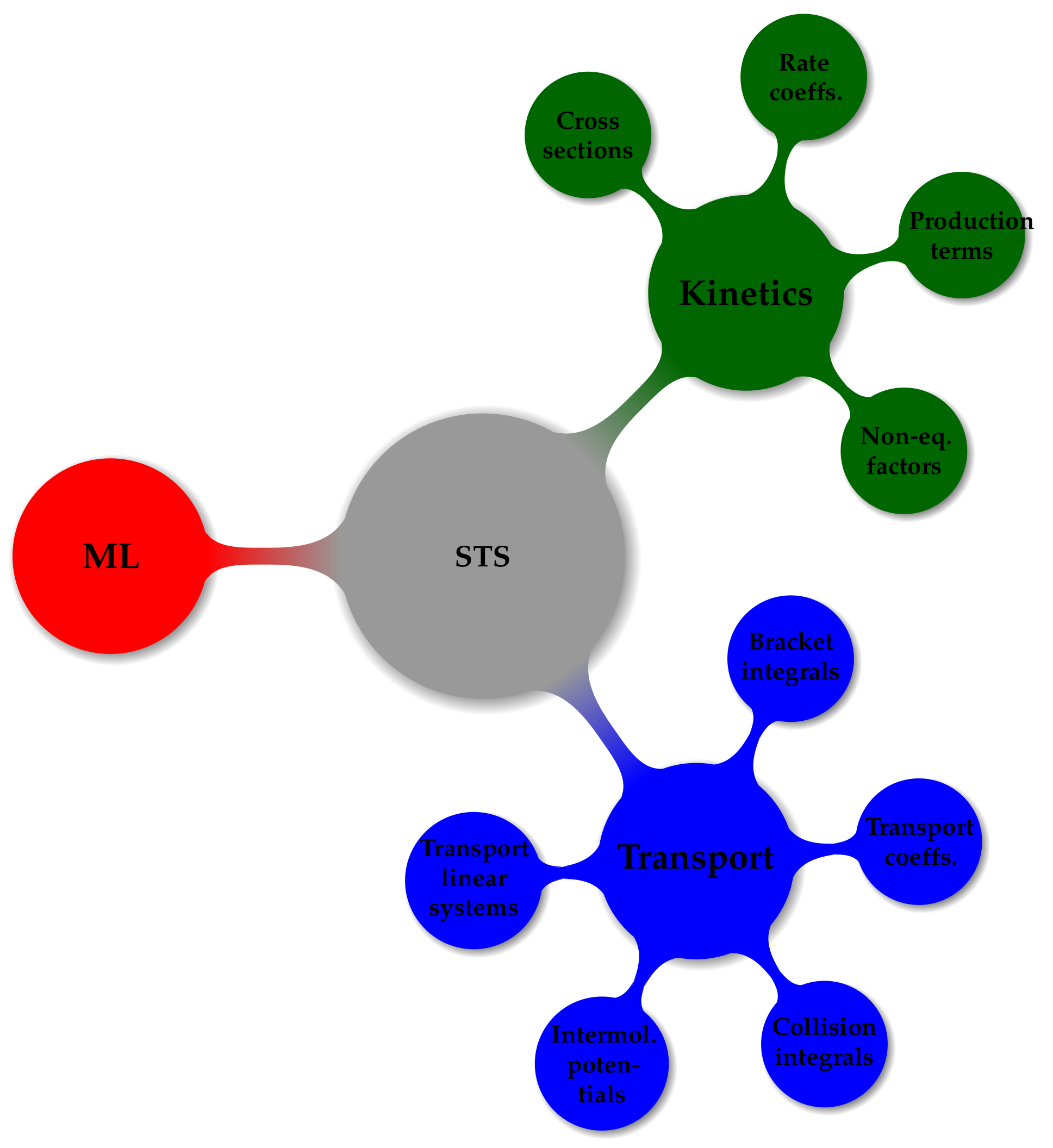
2. State-to-State Problem Formulation
3. Regression
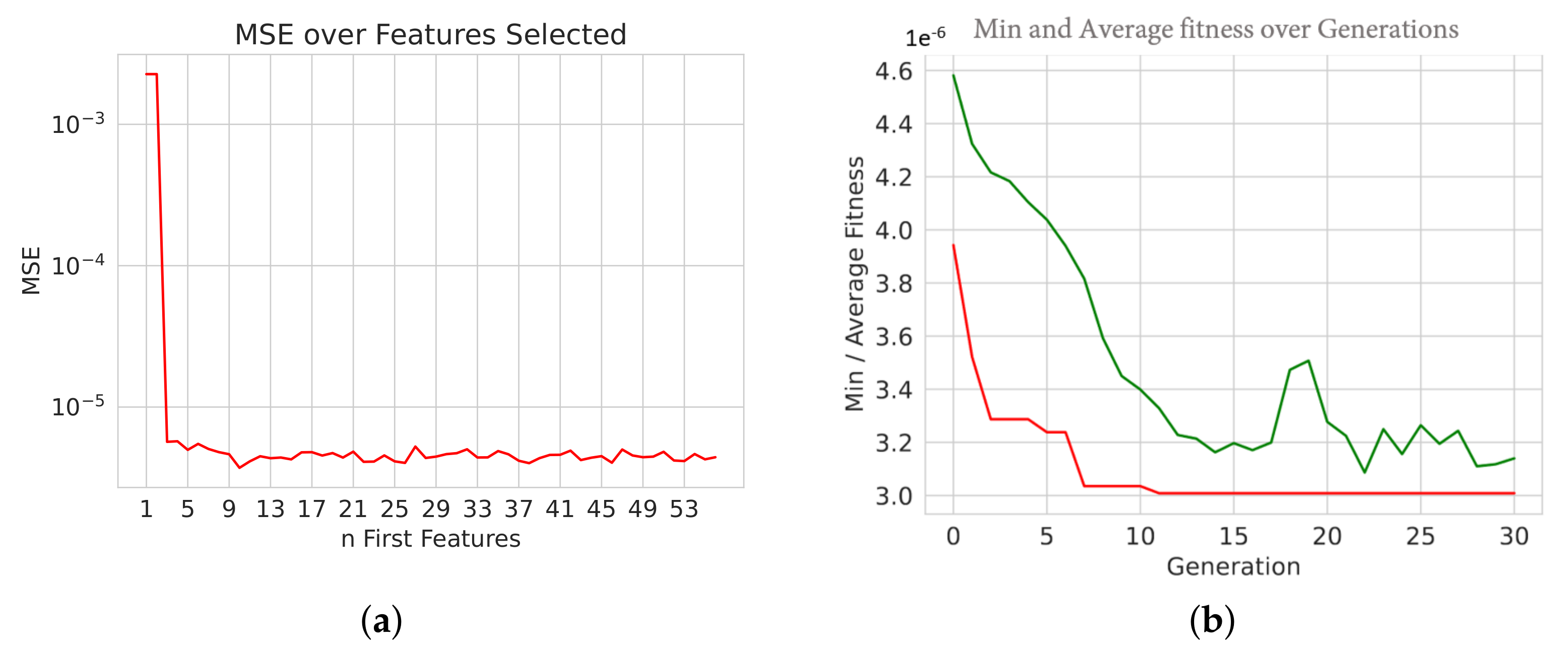
Genetic Algorithms
-- Best Ever Individual =  [1, 0, 0, 1, 1, 1, 1, 0, 1, 1, 0, 0,
1, 1, 0, 1, 0, 0, 1, 0, 0, 0, 1, 1, 0, 1, 0, 0, 1, 1, 1, 0, 0,
1, 1, 0, 1, 1, 1, 1, 1, 1, 0, 1, 1, 1, 1, 0, 0, 1, 0, 1, 0, 1, 1, 1]
-- Best Ever Fitness =  3.0083253440920882e-06
*** Default Regressor Hyperparameter values:
{learning_rate: 1.0, loss: linear, n_estimators: 50, random_state: 42}
Score with default values = 0.9980733620530691
Time Elapsed = 0.00024271011352539062~s
*** Performing Grid Search...
Best parameters: {learning_rate: 1.0, loss: square, n_estimators: 30}
Best score: 0.9987849200477441
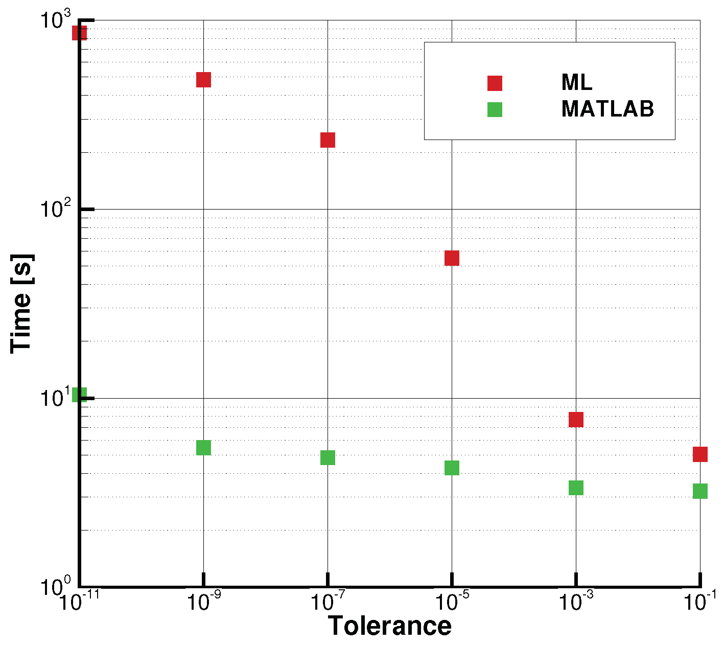
Time Elapsed = 1080.802133321762~s
*** Performing Genetic Grid Search...
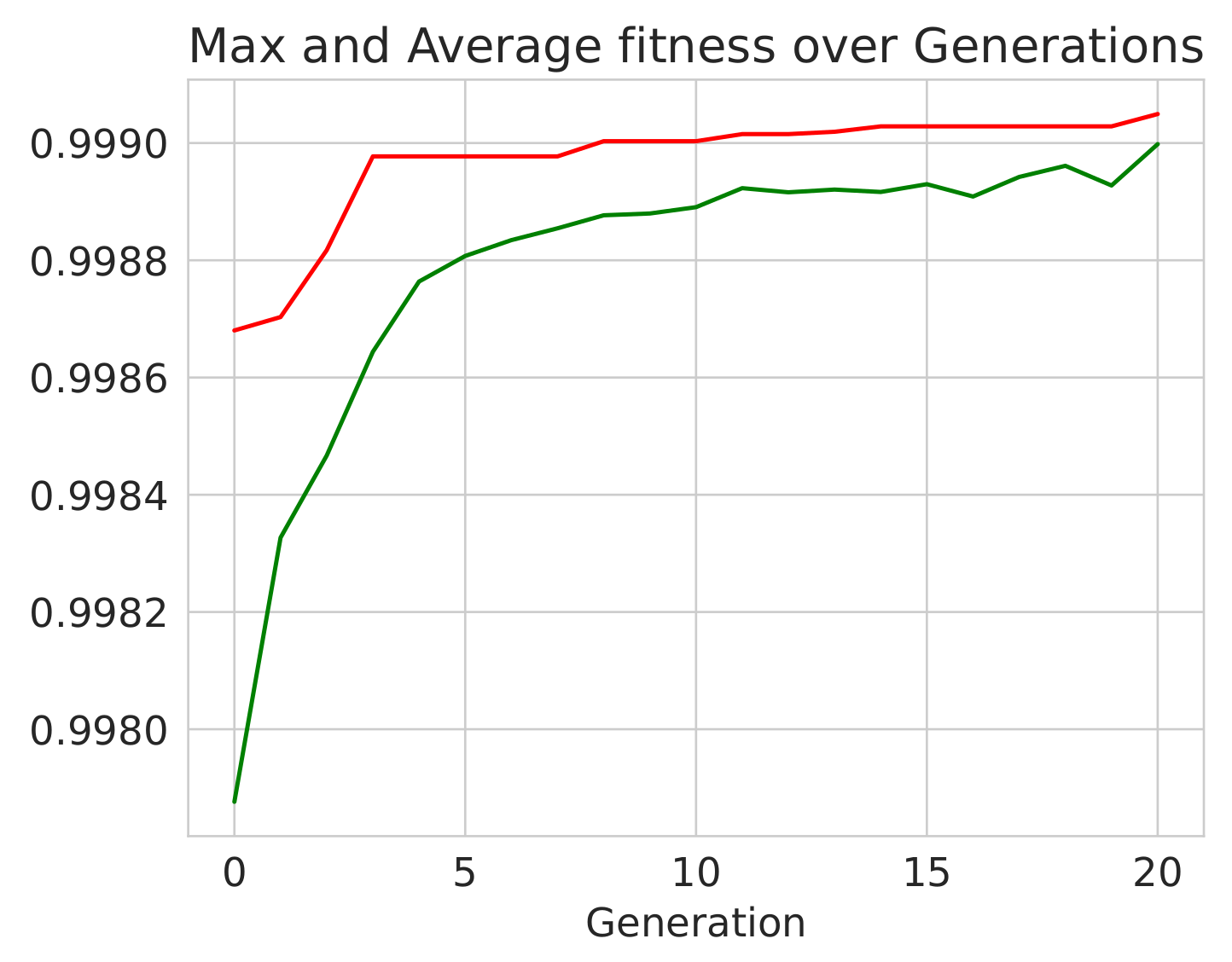
--- Evolve in 300 possible combinations ---
gen nevals avg min max std
0 20 0.997418 0.996355 0.998481 0.000614776
1 15 0.997736 0.996508 0.998611 0.000582864
2 11 0.997967 0.997001 0.998614 0.000521943
3 14 0.998238 0.997351 0.998682 0.000403602
4 12 0.998421 0.997624 0.998682 0.00032174
5 9 0.998547 0.997658 0.998682 0.000216111
Best individual is: {n_estimators: 80, learning_rate: 0.215, loss: square}
with fitness: 0.9986822271396701
Time Elapsed = 352.01691937446594 s
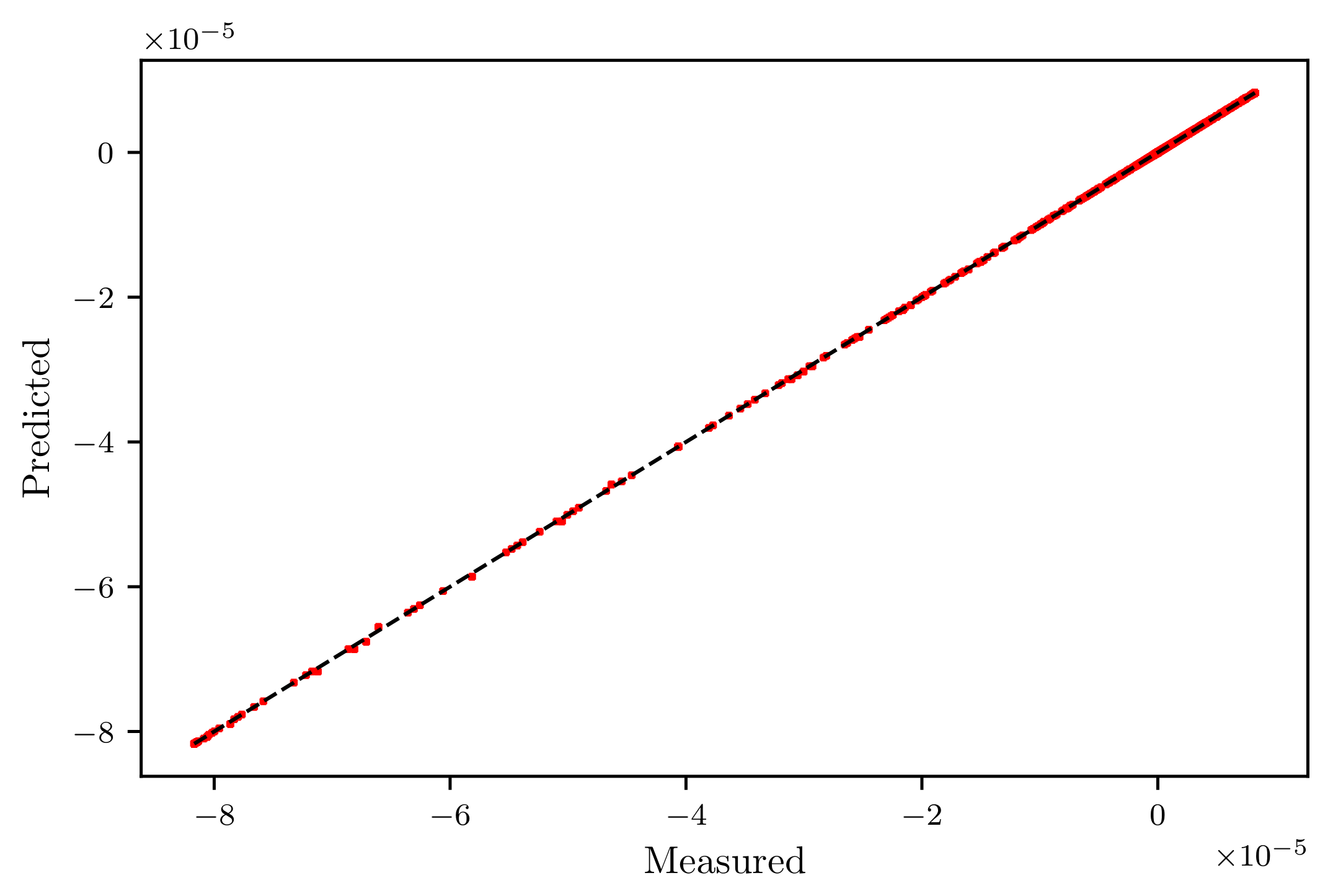
- Best solution is:
params = n_estimators = 25, learning_rate = 0.929, loss = square
Accuracy = 0.99900
4. Machine Learning Coupled with ODE Solver
4.1. Matlab-Python Interface
- Regression of chemical reaction rate coefficients, , (lines 5–8 of Algorithm A1);
- Regression of chemical reaction relaxation terms, , Equation (6) (lines 9–10 of Algorithm A1, before matrix inversion at line 12);
- Regression of the right-hand side inside ODE function call, (after matrix inversion at line 12 of (lines 5–8 of Algorithm A1);
- Regression of the ODE solver function call output, [X,Y] at line 2 of Listing A1).
4.2. Fortran-Python Interface
- Re-coding specific model architectures into Fortran;
- Calling Python from within Fortran (e.g., using wrapper libraries such as Python’s C API [70], Cython [71], CFFI (https://cffi.readthedocs.io), SWIG [72] (http://www.swig.org/projects.html), Babel [73], SIP (https://riverbankcomputing.com/software/sip/intro) or Boost.python library (https://wiki.python.org/moin/boost.python);
- Use a pure Fortran NN library, or bridging library (there are several existing solutions, e.g., FANN (https://github.com/libfann), neural-fortran (https://github.com/modern-fortran/neural-fortran), FKB (https://github.com/scientific-computing/FKB), frugally-deep (https://github.com/Dobiasd/frugally-deep), Ro-boDNN [74], TensorflowLite [64] C/C++ API and tiny-dnn (https://github.com/tiny-dnn/tiny-dnn), (all accessed on 1 March 2022);
- Intrinsic Fortran procedures, such as get_command_argument, get_command to invoke Python scripts and exchange data through I/O files.
- Create, train and save deep learning model from Python:model.save("keras_model.h5", include_optimizer=False);
- Convert the saved model into the required format:python3 convert_model.py keras_model.h5 fdeep_model.json;
- Load model in C++ using frugally-deep:const auto model = fdeep::load_model("fdeep_model.json");
- Load data from Fortran:
- -
- pass it to function in C++;
- -
- make inference;
- -
- pass inference result back to Fortran.
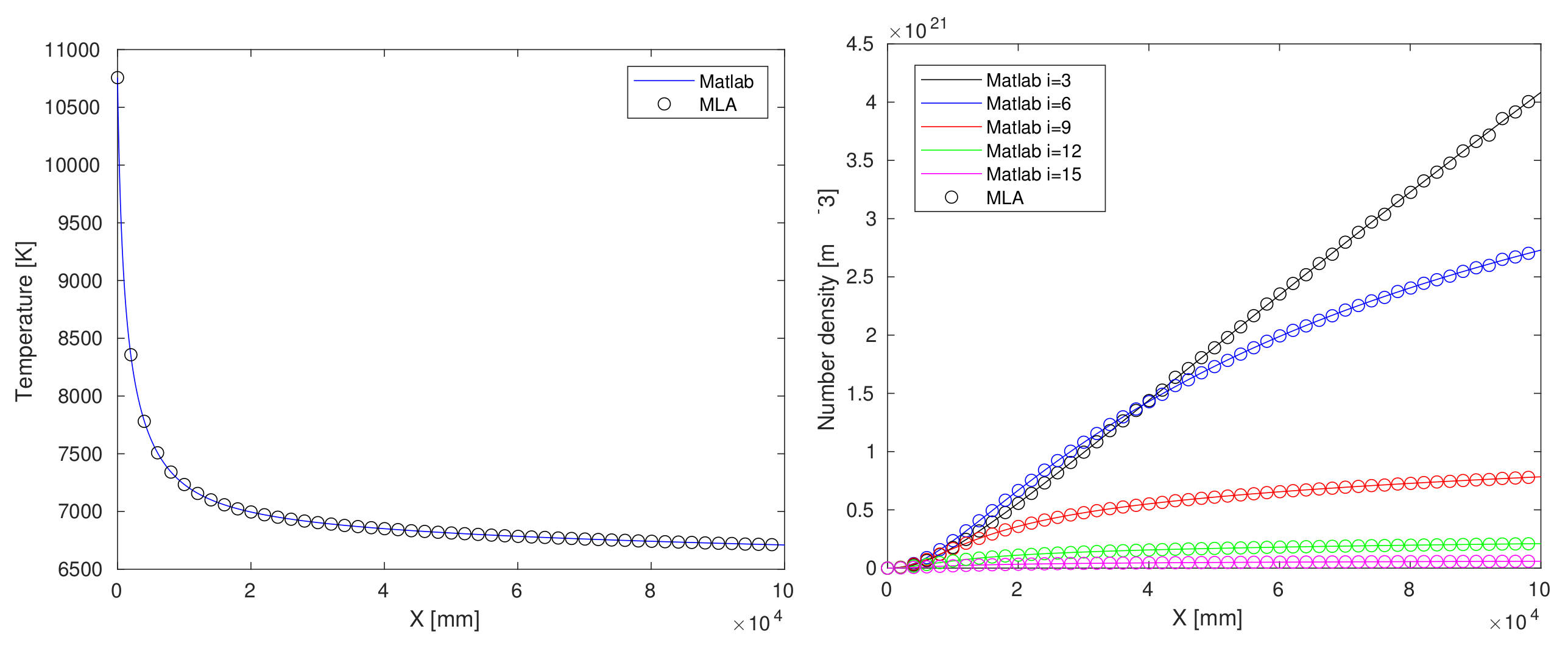
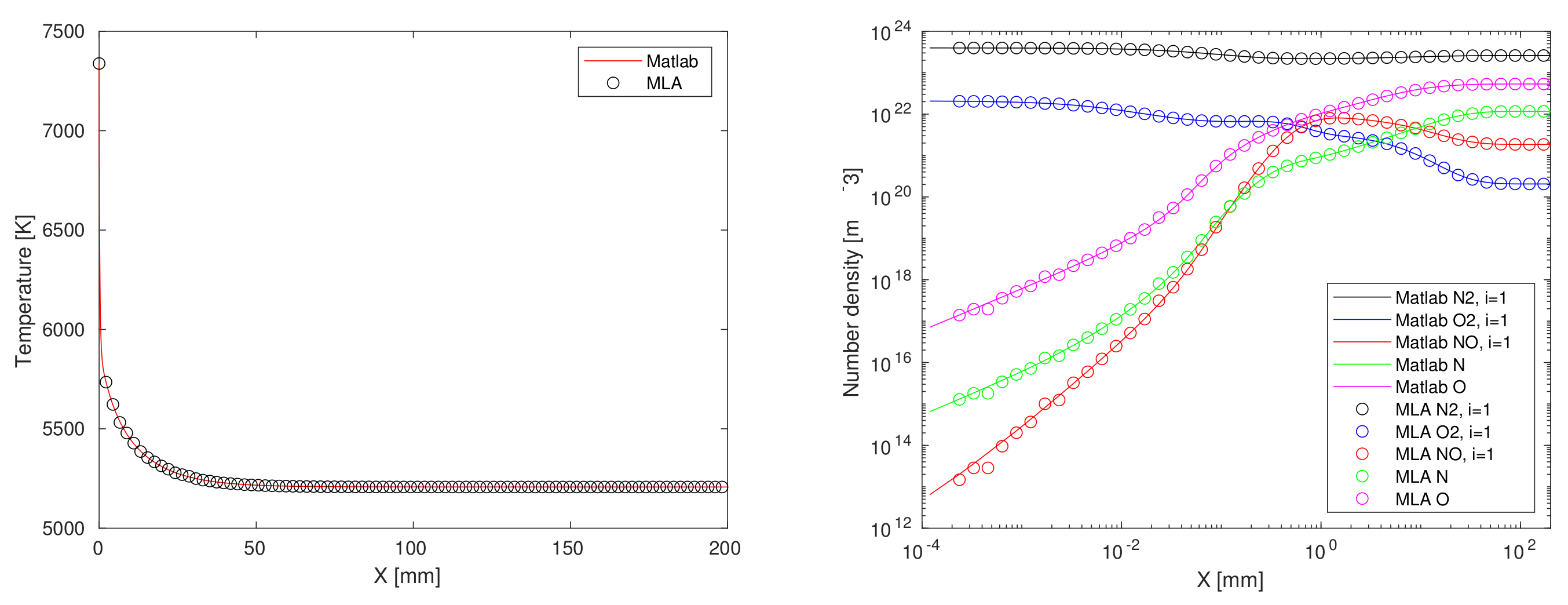
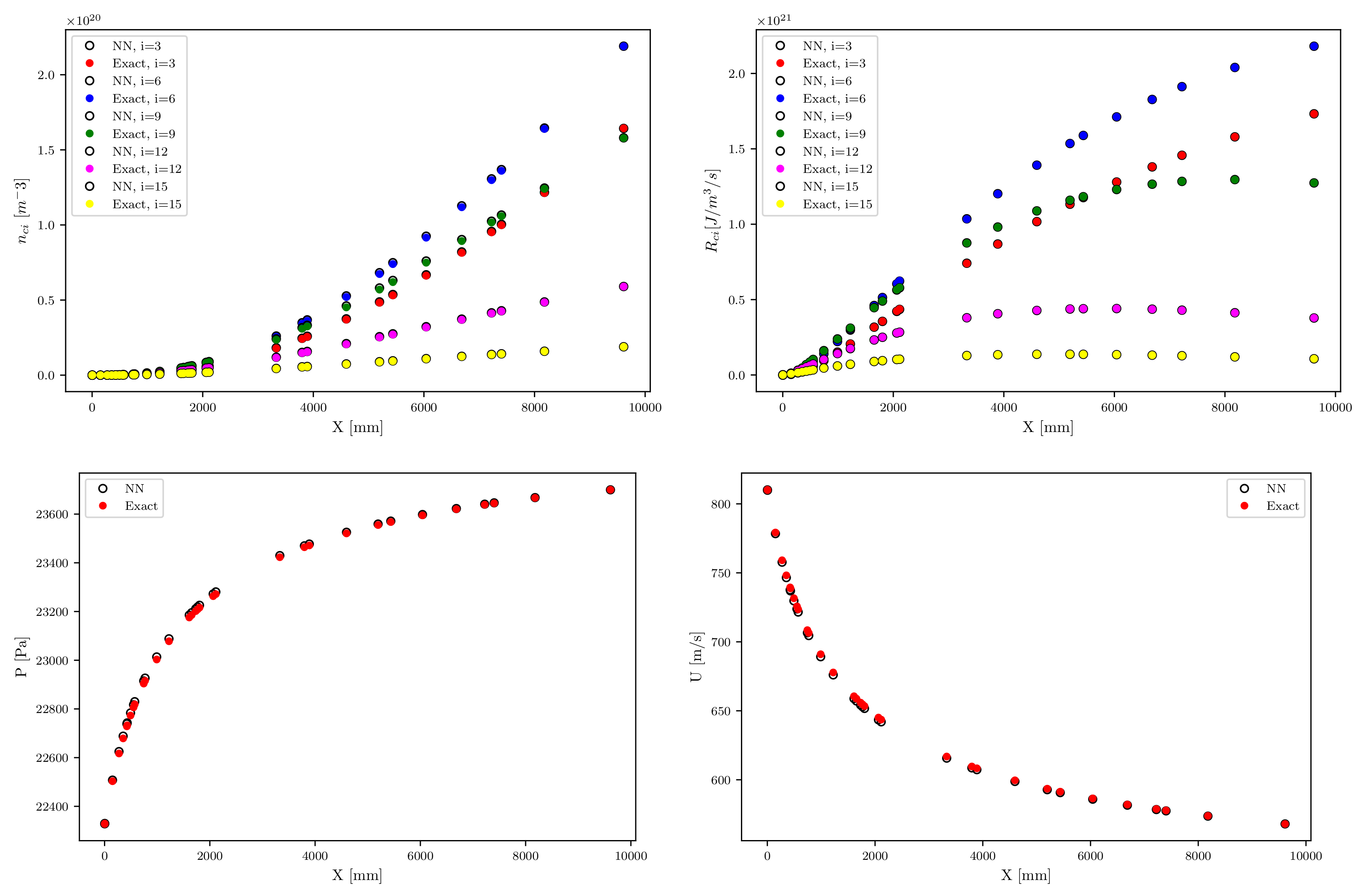
5. Deep Neural Network for 1D STS Euler Shock Flow Relaxation
6. Conclusions
Author Contributions
Funding
Acknowledgments
Conflicts of Interest
Appendix A. Machine Learning Coupled with ODE Solver—Matlab-Python Interface Code
      options = odeset('RelTol', 1e-12, 'AbsTol', 1e-12);
      [X,Y] = ode15s(@rpart, xspan, Y0_bar,options);
| Algorithm A1 Source term calculation. | |
| 1: function rpart() | |
| 2: compute A | ▹ A x = B |
| 3: compute | ▹ diss/rec eq. constant |
| 4: compute K | ▹ vibr/trans. eq. constant |
| 5: compute k | ▹ diss. rates |
| 6: compute k | ▹ rec. rates |
| 7: compute k | ▹ vibr/trans. rates |
| 8: compute k | ▹ vibr/vibr. rates |
| 9: for do | ▹ l, vibrational levels |
| ▹ dis./rec. source terms | |
| ▹ vibr./trans. source terms | |
| ▹ vibr./vibr. source terms | |
| 10: end for | |
| 11: | ▹ full source terms |
| 12: | |
| 13: return dy | |
| 14: end function | |
References
- Armenise, I.; Reynier, P.; Kustova, E. Advanced models for vibrational and chemical kinetics applied to Mars entry aerothermodynamics. J. Thermophys. Heat Transf. 2016, 30, 705–720. [Google Scholar] [CrossRef]
- Kunova, O.; Kustova, E.; Mekhonoshina, M.; Nagnibeda, E. Non-equilibrium kinetics, diffusion and heat transfer in shock heated flows of N2/N and O2/O mixtures. Chem. Phys. 2015, 463, 70–81. [Google Scholar] [CrossRef]
- Kunova, O.; Kustova, E.; Mekhonoshina, M.; Shoev, G. Numerical simulation of coupled state-to-state kinetics and heat transfer in viscous non-equilibrium flows. In AIP Conference Proceedings; AIP Publishing LLC: Melville, NY, USA, 2016; Volume 1786, p. 070012. [Google Scholar]
- Kunova, O.; Kosareva, A.; Kustova, E.; Nagnibeda, E. Vibrational relaxation of carbon dioxide in state-to-state and multi-temperature approaches. Phys. Rev. Fluids 2020, 5, 123401. [Google Scholar] [CrossRef]
- Magin, T.E.; Panesi, M.; Bourdon, A.; Jaffe, R.L.; Schwenke, D.W. Coarse-grain model for internal energy excitation and dissociation of molecular nitrogen. Chem. Phys. 2012, 398, 90–95. [Google Scholar] [CrossRef]
- Munafo, A.; Panesi, M.; Magin, T. Boltzmann rovibrational collisional coarse-grained model for internal energy excitation and dissociation in hypersonic flows. Phys. Rev. E 2014, 89, 023001. [Google Scholar] [CrossRef]
- Parsons, N.; Levin, D.A.; van Duin, A.C.; Zhu, T. Modeling of molecular nitrogen collisions and dissociation processes for direct simulation Monte Carlo. J. Chem. Phys. 2014, 141, 234307. [Google Scholar] [CrossRef]
- Torres, E.; Bondar, Y.A.; Magin, T. Uniform rovibrational collisional N2 bin model for DSMC, with application to atmospheric entry flows. In AIP Conference Proceedings; AIP Publishing LLC: Melville, NY, USA, 2016; Volume 1786, p. 050010. [Google Scholar]
- Berthelot, A.; Bogaerts, A. Modeling of plasma-based CO2 conversion: Lumping of the vibrational levels. Plasma Sources Sci. Technol. 2016, 25, 045022. [Google Scholar] [CrossRef]
- Sahai, A.; Lopez, B.E.; Johnston, C.O.; Panesi, M. A reduced order maximum entropy model for chemical and thermal non-equilibrium in high temperature CO2 gas. In Proceedings of the 46th AIAA Thermophysics Conference, Washington, DC, USA, 13–17 June 2016; p. 3695. [Google Scholar]
- Diomede, P.; van den Sanden, M.C.; Longo, S. Insight into CO2 dissociation in plasma from numerical solution of a vibrational diffusion equation. J. Phys. Chem. C 2017, 121, 19568–19576. [Google Scholar] [CrossRef] [Green Version]
- Bonelli, F.; Tuttafesta, M.; Colonna, G.; Cutrone, L.; Pascazio, G. An MPI-CUDA approach for hypersonic flows with detailed state-to-state air kinetics using a GPU cluster. Comput. Phys. Commun. 2017, 219, 178–195. [Google Scholar] [CrossRef]
- Armenise, I.; Capitelli, M.; Garcia, E.; Gorse, C.; Lagana, A.; Longo, S. Deactivation dynamics of vibrationally excited nitrogen molecules by nitrogen atoms. Effects on non-equilibrium vibrational distribution and dissociation rates of nitrogen under electrical discharges. Chem. Phys. Lett. 1992, 200, 597–604. [Google Scholar] [CrossRef]
- Longo, S.; Comunale, G.; Gorse, C.; Capitelli, M. Simplified and complex modeling of self-sustained discharge-pumped, Ne-buffered XeCl laser kinetics. Plasma Chem. Plasma Process. 1993, 13, 685–700. [Google Scholar] [CrossRef]
- Morgan, W.L. The feasibility of using neural networks to obtain cross sections from electron swarm data. IEEE Trans. Plasma Sci. 1991, 19, 250–255. [Google Scholar] [CrossRef]
- Tezcan, S.; Akcayol, M.; Ozerdem, O.C.; Dincer, M. Calculation of Electron Energy Distribution Functions From Electron Swarm Parameters Using Artificial Neural Network in SF6 and Argon. IEEE Trans. Plasma Sci. 2010, 38, 2332–2339. [Google Scholar] [CrossRef]
- Stokes, P.W.; Cocks, D.G.; Brunger, M.J.; White, R.D. Determining cross sections from transport coefficients using deep neural networks. Plasma Sources Sci. Technol. 2020, 29, 055009. [Google Scholar] [CrossRef] [Green Version]
- Schmidt, J.; Marques, M.R.; Botti, S.; Marques, M.A. Recent advances and applications of machine learning in solid-state materials science. Npj Comput. Mater. 2019, 5, 1–36. [Google Scholar]
- Brunton, S.L.; Noack, B.R.; Koumoutsakos, P. Machine learning for fluid mechanics. Annu. Rev. Fluid Mech. 2020, 52, 477–508. [Google Scholar] [CrossRef] [Green Version]
- Bruno, D.; Capitelli, M.; Catalfamo, C.; Celiberto, R.; Colonna, G.; Diomede, P.; Giordano, D.; Gorse, C.; Laricchiuta, A.; Longo, S.; et al. Transport properties of high-temperature Mars-atmosphere components. ESA Sci. Tech. Rev. 2008, 256. [Google Scholar] [CrossRef]
- Brunton, S.L.; Hemati, M.S.; Taira, K. Special issue on machine learning and data-driven methods in fluid dynamics. Theor. Comput. Fluid Dyn. 2020, 34, 333–337. [Google Scholar] [CrossRef]
- Gupta, R.N.; Yos, J.M.; Thompson, R.A.; Lee, K.P. A Review of Reaction Rates and Thermodynamic and Transport Properties for an 570 11-Species Air Model for Chemical and Thermal Nonequilibrium Calculations to 30000 K; NASA Technical Report NASA-RP-1232; National Aeronautics and Space Administration, Langley Research Center: Hampton, VA, USA, 1990; Volume 90.
- Nagnibeda, E.; Kustova, E. Nonequilibrium Reacting Gas Flows. Kinetic Theory of Transport and Relaxation Processes; Springer: Berlin/Heidelberg, Germany, 2009. [Google Scholar]
- Stupochenko, Y.; Losev, S.; Osipov, A. Relaxation Processes in Shock Waves; Springer: Berlin/Heidelberg, Germany, 1967. [Google Scholar]
- Kunova, O.; Nagnibeda, E. State-to-state description of reacting air flows behind shock waves. Chem. Phys. 2014, 441, 66–76. [Google Scholar] [CrossRef]
- Campoli, L.; Kunova, O.; Kustova, E.; Melnik, M. Models validation and code profiling in state-to-state simulations of shock heated air flows. Acta Astronaut. 2020, 175, 493–509. [Google Scholar] [CrossRef]
- Schwartz, R.; Slawsky, Z.; Herzfeld, K. Calculation of Vibrational Relaxation Times in Gases. J. Chem. Phys. 1952, 20, 1591–1599. [Google Scholar] [CrossRef]
- Herzfeld, K.; Litovitz, T. Absorption and Dispersion of Ultrasonic Waves; Academic Press: Cambridge, MA, USA, 2013; Volume 7. [Google Scholar]
- Marrone, P.; Treanor, C. Chemical Relaxation with Preferential Dissociation from Excited Vibrational Levels. Phys. Fluids 1963, 6, 1215–1221. [Google Scholar] [CrossRef]
- Kunova, O.; Kustova, E.; Savelev, A. Generalized Treanor–Marrone model for state-specific dissociation rate coefficients. Chem. Phys. Lett. 2016, 659, 80–87. [Google Scholar] [CrossRef]
- Adamovich, I.; Macheret, S.; Rich, J.; Treanor, C. Vibrational energy transfer rates using a forced harmonic oscillator model. J. Thermophys. Heat Transfer. 1998, 12, 57–65. [Google Scholar] [CrossRef]
- Kustova, E.; Savelev, A.; Kunova, O. Rate coefficients of exchange reactions accounting for vibrational excitation of reagents and products. AIP Conf. Proc. 2018, 1959, 060010. [Google Scholar]
- Aliat, A. State-to-state dissociation-recombination and chemical exchange rate coefficients in excited diatomic gas flows. Phys. A: Stat. Mech. Its Appl. 2008, 387, 4163–4182. [Google Scholar] [CrossRef]
- Park, C. Review of chemical-kinetic problems of future NASA missions. I-Earth entries. J. Thermophys. Heat Transf. 1993, 7, 385–398. [Google Scholar] [CrossRef]
- Brunton, S.L.; Kutz, J.N. Data-Driven Science and Engineering: Machine Learning, Dynamical Systems, and Control; Cambridge University Press: Cambridge, UK, 2019. [Google Scholar]
- Rasmussen, C.E. Gaussian Processes in Machine Learning; Summer School on Machine Learning; Springer: Berlin/Heidelberg, Germany, 2003; pp. 63–71. [Google Scholar]
- Stulp, F.; Sigaud, O. Many regression algorithms, one unified model: A review. Neural Netw. 2015, 69, 60–79. [Google Scholar] [CrossRef] [PubMed] [Green Version]
- Kostopoulos, G.; Karlos, S.; Kotsiantis, S.; Ragos, O. Semi-supervised regression: A recent review. J. Intell. Fuzzy Syst. 2018, 35, 1483–1500. [Google Scholar] [CrossRef]
- Pedregosa, F.; Varoquaux, G.; Gramfort, A.; Michel, V.; Thirion, B.; Grisel, O.; Blondel, M.; Prettenhofer, P.; Weiss, R.; Dubourg, V.; et al. Scikit-learn: Machine learning in Python. J. Mach. Learn. Res. 2011, 12, 2825–2830. [Google Scholar]
- Campoli, L. Machine learning methods for state-to-state approach. In AIP Conference Proceedings; AIP Publishing LLC: Melville, NY, USA, 2021; Volume 2351, p. 030041. [Google Scholar]
- Kelp, M.M.; Tessum, C.W.; Marshall, J.D. Orders-of-magnitude speedup in atmospheric chemistry modeling through neural network-based emulation. arXiv 2018, arXiv:1808.03874. [Google Scholar]
- Wan, K.; Barnaud, C.; Vervisch, L.; Domingo, P. Chemistry reduction using machine learning trained from non-premixed micro-mixing modeling: Application to DNS of a syngas turbulent oxy-flame with side-wall effects. Combust. Flame 2020, 220, 119–129. [Google Scholar] [CrossRef]
- Zhang, T.; Zhang, Y.; E, W.; Ju, Y. DLODE: A deep learning-based ODE solver for chemistry kinetics. In Proceedings of the AIAA Scitech 2021 Forum, virtual event. 11–15 & 19–21 January 2021; p. 1139. [Google Scholar]
- Holland, J.H. Genetic algorithms. Sci. Am. 1992, 267, 66–73. [Google Scholar] [CrossRef]
- Koza, J.R. Survey of genetic algorithms and genetic programming. In Wescon Conference Record; Western Periodicals Company: Racine, WI, USA, 1995; pp. 589–594. [Google Scholar]
- Mitchell, M. An Introduction to Genetic Algorithms; MIT Press: Cambridge, MA, USA, 1998. [Google Scholar]
- Goldberg, D.E. Genetic Algorithms; Pearson Education India: London, UK, 2006. [Google Scholar]
- Koza, J.R. Genetic Programming II: Automatic Discovery of Reusable Programs; MIT Press: Cambridge, MA, USA, 1994. [Google Scholar]
- Guyon, I.; Gunn, S.; Nikravesh, M.; Zadeh, L.A. Feature Extraction: Foundations and Applications; Springer: Berlin/Heidelberg, Germany, 2008; Volume 207. [Google Scholar]
- Chandrashekar, G.; Sahin, F. A survey on feature selection methods. Comput. Electr. Eng. 2014, 40, 16–28. [Google Scholar] [CrossRef]
- Kumar, V.; Minz, S. Feature selection: A literature review. SmartCR 2014, 4, 211–229. [Google Scholar] [CrossRef]
- Li, J.; Cheng, K.; Wang, S.; Morstatter, F.; Trevino, R.P.; Tang, J.; Liu, H. Feature selection: A data perspective. ACM Comput. Surv. (CSUR) 2017, 50, 1–45. [Google Scholar] [CrossRef]
- Cunningham, P.; Kathirgamanathan, B.; Delany, S.J. Feature Selection Tutorial with Python Examples. arXiv 2021, arXiv:2106.06437. [Google Scholar]
- Bolón-Canedo, V.; Sánchez-Maroño, N.; Alonso-Betanzos, A. A review of feature selection methods on synthetic data. Knowl. Inf. Syst. 2013, 34, 483–519. [Google Scholar] [CrossRef]
- Vafaie, H.; De Jong, K.A. Genetic Algorithms as a Tool for Feature Selection in Machine Learning. In Proceedings of the International Conference on Tools with Artificial Intelligence—ICTAI, Arlington, VA, USA, 10–13 November 1992; pp. 200–203. [Google Scholar]
- Fortin, F.A.; De Rainville, F.M.; Gardner, M.A.G.; Parizeau, M.; Gagné, C. DEAP: Evolutionary algorithms made easy. J. Mach. Learn. Res. 2012, 13, 2171–2175. [Google Scholar]
- Zhong, J.; Feng, L.; Ong, Y.S. Gene expression programming: A survey. IEEE Comput. Intell. Mag. 2017, 12, 54–72. [Google Scholar] [CrossRef]
- Vaddireddy, H.; San, O. Equation discovery using fast function extraction: A deterministic symbolic regression approach. Fluids 2019, 4, 111. [Google Scholar] [CrossRef] [Green Version]
- Vaddireddy, H.; Rasheed, A.; Staples, A.E.; San, O. Feature engineering and symbolic regression methods for detecting hidden physics from sparse sensor observation data. Phys. Fluids 2020, 32, 015113. [Google Scholar] [CrossRef] [Green Version]
- Blasco, J.A.; Fueyo, N.; Larroya, J.; Dopazo, C.; Chen, Y.J. A single-step time-integrator of a methane–air chemical system using artificial neural networks. Comput. Chem. Eng. 1999, 23, 1127–1133. [Google Scholar] [CrossRef]
- Buchheit, K.; Owoyele, O.; Jordan, T.; Van Essendelft, D. The Stabilized Explicit Variable-Load Solver with Machine Learning Acceleration for the Rapid Solution of Stiff Chemical Kinetics. arXiv 2019, arXiv:1905.09395. [Google Scholar]
- Chen, R.T.; Rubanova, Y.; Bettencourt, J.; Duvenaud, D.K. Neural ordinary differential equations. Adv. Neural Inf. Process. Syst. 2018, 31, 6571–6583. [Google Scholar]
- Rackauckas, C.; Innes, M.; Ma, Y.; Bettencourt, J.; White, L.; Dixit, V. Diffeqflux. jl-A julia library for neural differential equations. arXiv 2019, arXiv:1902.02376. [Google Scholar]
- Abadi, M.; Agarwal, A.; Barham, P.; Brevdo, E.; Chen, Z.; Citro, C.; Corrado, G.S.; Davis, A.; Dean, J.; Devin, M.; et al. Tensorflow: Large-scale machine learning on heterogeneous distributed systems. arXiv 2016, arXiv:1603.04467. [Google Scholar]
- Paszke, A.; Gross, S.; Massa, F.; Lerer, A.; Bradbury, J.; Chanan, G.; Killeen, T.; Lin, Z.; Gimelshein, N.; Antiga, L.; et al. Pytorch: An imperative style, high-performance deep learning library. Adv. Neural Inf. Process. Syst. 2019, 32, 8026–8037. [Google Scholar]
- Jia, Y.; Shelhamer, E.; Donahue, J.; Karayev, S.; Long, J.; Girshick, R.; Guadarrama, S.; Darrell, T. Caffe: Convolutional architecture for fast feature embedding. In Proceedings of the 22nd ACM International Conference on Multimedia, Orlando, FL, USA, 3–7 November 2014; pp. 675–678. [Google Scholar]
- Chen, T.; Li, M.; Li, Y.; Lin, M.; Wang, N.; Wang, M.; Xiao, T.; Xu, B.; Zhang, C.; Zhang, Z. Mxnet: A flexible and efficient machine learning library for heterogeneous distributed systems. arXiv 2015, arXiv:1512.01274. [Google Scholar]
- Al-Rfou, R.; Alain, G.; Almahairi, A.; Angermueller, C.; Bahdanau, D.; Ballas, N.; Bastien, F.; Bayer, J.; Belikov, A.; Belopolsky, A.; et al. Theano: A Python framework for fast computation of mathematical expressions. arXiv 2016, arXiv:1605.02688. [Google Scholar]
- Wang, Y.; Reddy, R.; Gomez, R.; Lim, J.; Sanielevici, S.; Ray, J.; Sutherland, J.; Chen, J. A General Approach to Creating Fortran Interface for C++ Application Libraries. In Current Trends in High Performance Computing and Its Applications; Springer: Berlin/Heidelberg, Germany, 2005; pp. 145–154. [Google Scholar]
- Van Rossum, G.; Drake, F.L., Jr. Python/C API Reference Manual; Python Software Foundation: Wilmington, DE, USA, 2002. [Google Scholar]
- Behnel, S.; Bradshaw, R.; Citro, C.; Dalcin, L.; Seljebotn, D.S.; Smith, K. Cython: The best of both worlds. Comput. Sci. Eng. 2011, 13, 31–39. [Google Scholar] [CrossRef]
- Beazley, D.M. SWIG: An Easy to Use Tool for Integrating Scripting Languages with C and C++. In Proceedings of the Tcl/Tk Workshop, Monterey, CA, USA, 10–13 July 1996; Volume 43, p. 74. [Google Scholar]
- Prantl, A.; Epperly, T.; Imam, S.; Sarkar, V. Interfacing Chapel with Traditional HPC Programming Languages; Technical Report; Lawrence Livermore National Lab. (LLNL): Livermore, CA, USA, 2011. [Google Scholar]
- Szemenyei, M.; Estivill-Castro, V. Real-time scene understanding using deep neural networks for RoboCup SPL. In Robot World Cup; Springer: Berlin/Heidelberg, Germany, 2018; pp. 96–108. [Google Scholar]
- Johnson, S.R.; Prokopenko, A.; Evans, K.J. Automated Fortran–C++ Bindings for Large-Scale Scientific Applications. Comput. Sci. Eng. 2019, 22, 84–94. [Google Scholar] [CrossRef] [Green Version]
- Prokopenko, A.V.; Johnson, S.R.; Bement, M.T. Documenting Automated Fortran-C++ Bindings with SWIG; Technical Report; Oak Ridge National Lab. (ORNL): Oak Ridge, TN, USA, 2019. [Google Scholar]
- Evans, K.; Young, M.; Collins, B.; Johnson, S.; Prokopenko, A.; Heroux, M. Existing Fortran Interfaces to Trilinos in Preparation for Exascale ForTrilinos Development; Technical Report; Oak Ridge National Lab. (ORNL): Oak Ridge, TN, USA, 2017. [Google Scholar]
- Young, M.T.; Johnson, S.R.; Prokopenko, A.V.; Evans, K.J.; Heroux, M.A. ForTrilinos Design Document; Technical Report; Oak Ridge National Lab. (ORNL): Oak Ridge, TN, USA, 2017. [Google Scholar]
- Mao, Z.; Lu, L.; Marxen, O.; Zaki, T.A.; Karniadakis, G.E. DeepM&Mnet for hypersonics: Predicting the coupled flow and finite-rate chemistry behind a normal shock using neural-network approximation of operators. arXiv 2020, arXiv:2011.03349. [Google Scholar]
- Cai, S.; Wang, Z.; Lu, L.; Zaki, T.A.; Karniadakis, G.E. DeepM&Mnet: Inferring the electroconvection multiphysics fields based on operator approximation by neural networks. arXiv 2020, arXiv:2009.12935. [Google Scholar]
- Sharma, A.J.; Johnson, R.F.; Kessler, D.A.; Moses, A. Deep Learning for Scalable Chemical Kinetics. In Proceedings of the AIAA Scitech 2020 Forum, Orlando, FL, USA, 6–10 January 2020; p. 0181. [Google Scholar] [CrossRef]

| Key | Value |
| Flow Type | Navier_Stokes |
| Species | N2, O2, NO, N, O |
| Kinetic | STS |
| Transport | Gupta |
| Gas Model | Nonequ_Gas |
| Simulation_Type | 2D_AXI |
| Pressure | 2.0 |
| Temperature | 195.0 |
| Velocity | 11,360.0 |
| Mass Fractions | N2: 0.79, O2: 0.21 |
| Process | Time |
| Exchange | 0.00% |
| Update | 0.26% |
| ComputeConvectionFlux | 1.51% |
| ComputeDissipationFlux | 21.93% |
| ComputeSourceTerms | 76.27% |
| ComputeLocalResidual | 0.01% |
| Algorithm | Parameter | Values |
|---|---|---|
| KR | kernel | {poly, rbf} |
| alpha | {1e-3, 1e-2, 1e-1, 1e0, 1e1, 1e2, 1e3} | |
| gamma | {1e-3, 1e-2, 1e-1, 1e0, 1e1, 1e2, 1e3} | |
| SVM | kernel | {poly, rbf} |
| gamma | {scale, auto} | |
| C | {1e-2, 1e-1, 1e0, 1e1, 1e2} | |
| epsilon | {1e-3, 1e-2, 1e-1, 1e0, 1e1, 1e2, 1e3} | |
| coef0 | {1e0, 1e-1, 2e-1} | |
| kNN | algorithm | {ball_tree, kd_tree, brute} |
| n_neighbors | {1,2,3,4,5,6,7,8,9,10} | |
| leaf_size | {1, 10, 20, 30, 100} | |
| weights | {uniform, distance} | |
| p | {1, 2} | |
| GP | n_restarts_optimizer | {(0,1,10,100} |
| alpha | {1e-3, 1e-2, 1e-1, 1e0, 1e1, 1e2, 1e3} | |
| kernel | {RBF, ExpSineSquared, RationalQuadratic, Matern} | |
| DT | criterion | {mse, friedman_mse, mae} |
| splitter | {best, random} | |
| max_features | {auto, sqrt, log2} | |
| RF | n_estimators | {10, 100, 1000} |
| min_weight_fraction_leaf | {0.0, 0.1, 0.2, 0.3, 0.4, 0.5} | |
| max_features | {sqrt, log2, auto} | |
| criterion | {mse, mae} | |
| min_samples_leaf | {1, 2 ,3, 4, 5, 10, 100} | |
| bootstrap | {True, False} | |
| warm_start | {True, False} | |
| max_impurity_decrease | {0.1, 0.2, 0.3, 0.4, 0.5} | |
| ET | n_estimators | {10, 100, 1000} |
| min_weight_fraction_leaf | {0.0, 0.25, 0.5} | |
| max_depth | {1, 10, 100, None} | |
| max_leaf_nodes | {2, 10, 100} | |
| min_samples_split | {2, 10, 100} | |
| min_samples_leaf | {1, 10, 100} | |
| GB | n_estimators | {10, 100, 1000} |
| min_weight_fraction_leaf | {0.0, 0.1, 0.2, 0.3, 0.4, 0.5} | |
| max_features | {sqrt, log2, auto, None} | |
| warm_start | {True, False} | |
| max_depth | {1, 10, 100, None} | |
| criterion | {friedman_mse, mse, mae} | |
| min_samples_split | {2, 5, 10} | |
| min_samples_leaf | {1, 10, 100} | |
| loss | {ls, lad, huber, quantile} | |
| HGB | loss | {least_squares, least_absolute_deviation, poisson} |
| min_sample_leaf | {1, 5, 10, 15, 20, 25, 50, 100} | |
| warm_start | {True, False} | |
| MLP | activation | {tanh, relu} |
| hidden_layer_sizes | {10, 50, 100, 150, 200} | |
| solver | {lbfgs, adam, sgd} | |
| leaning_rate | {constant, invscaling, adaptive} | |
| nesterovs_momentum | {True, False} | |
| warm_start | {True, False} | |
| early_stopping | {True, False} | |
| alpha | {0.00001, 0.0001, 0.001, 0.01, 0.1, 0.0} |
| Algorithm | MAE | MSE | RMSE | R2 | ||
|---|---|---|---|---|---|---|
| KR | 7.868505e-08 | 3.800217e-14 | 1.949414e-07 | 0.999999 | 7.612628 | 0.075077 |
| SVM | 1.236652e-02 | 2.109761e-04 | 1.452501e-02 | 0.999786 | 5.317098 | 0.008577 |
| kNN | 8.655485e-04 | 2.659352e-06 | 1.630752e-03 | 0.999997 | 0.002296 | 0.004962 |
| GP | 7.235743e-07 | 2.436803e-12 | 1.561026e-06 | 0.999994 | 118.3911 | 0.098444 |
| DT | 2.417524e-03 | 1.623255e-05 | 4.028964e-03 | 0.999983 | 0.003520 | 0.000317 |
| RF | 1.140677e-03 | 5.016757e-06 | 2.239812e-03 | 0.999992 | 4.362630 | 0.038143 |
| ET | 1.595557e-03 | 6.005923e-06 | 2.450698e-03 | 0.999993 | 2.279543 | 0.202767 |
| GB | 2.300499e-03 | 1.478234e-05 | 3.844782e-03 | 0.999985 | 4.823793 | 0.006213 |
| HGB | 6.098571e-03 | 1.395461e-04 | 1.181296e-02 | 0.999859 | 14.385128 | 0.042188 |
| MLP | 6.023895e-03 | 7.539429e-05 | 8.682989e-03 | 0.999943 | 11.322764 | 0.009778 |
| N2/N | air5 | |||||
|---|---|---|---|---|---|---|
| Matlab | ML | FANN | Matlab | ML | FANN | |
| Time [s] | 7.3541 | 6.8475 | 0.09 | 1874.7 | 6.8974 | 0.11 |
| Variable | Mean Relative Error |
|---|---|
| [m−3] | 4.890 × 10⁻⁴ |
| [J/m3/s] | 4.039 × 10⁻⁴ |
| [kg/m3] | 3.793 × 10⁻⁴ |
| u [m/s] | 3.673 × 10⁻⁴ |
| p [Pa] | 1.083 × 10⁻⁴ |
| E [eV] | 1.248 × 10⁻⁴ |
Publisher’s Note: MDPI stays neutral with regard to jurisdictional claims in published maps and institutional affiliations. |
© 2022 by the authors. Licensee MDPI, Basel, Switzerland. This article is an open access article distributed under the terms and conditions of the Creative Commons Attribution (CC BY) license (https://creativecommons.org/licenses/by/4.0/).
Share and Cite
Campoli, L.; Kustova, E.; Maltseva, P. Assessment of Machine Learning Methods for State-to-State Approach in Nonequilibrium Flow Simulations. Mathematics 2022, 10, 928. https://doi.org/10.3390/math10060928
Campoli L, Kustova E, Maltseva P. Assessment of Machine Learning Methods for State-to-State Approach in Nonequilibrium Flow Simulations. Mathematics. 2022; 10(6):928. https://doi.org/10.3390/math10060928
Chicago/Turabian StyleCampoli, Lorenzo, Elena Kustova, and Polina Maltseva. 2022. "Assessment of Machine Learning Methods for State-to-State Approach in Nonequilibrium Flow Simulations" Mathematics 10, no. 6: 928. https://doi.org/10.3390/math10060928
APA StyleCampoli, L., Kustova, E., & Maltseva, P. (2022). Assessment of Machine Learning Methods for State-to-State Approach in Nonequilibrium Flow Simulations. Mathematics, 10(6), 928. https://doi.org/10.3390/math10060928