The Adjoint Variable Method for Computational Electromagnetics

Abstract

Optimization using finite element analysis and the adjoint variable method to solve engineering problems appears in various application areas. However, to the best of the authors’ knowledge, there is a lack of detailed explanation on the implementation of the adjoint variable method in the context of electromagnetic modeling. This paper aimed to provide a detailed explanation of the method in the simplest possible general framework. Then, an extended explanation is offered in the context of electromagnetism. A discrete design methodology based on adjoint variables for magnetostatics was formulated, implemented, and verified. This comprehensive methodology supports both linear and nonlinear problems. The framework provides a general approach for performing a very efficient and discretely consistent sensitivity analysis for problems involving geometric and physical variables or any combination of the two. The accuracy of the implementation is demonstrated by independent verification based on an analytical test case and using the finite-difference method. The methodology was used to optimize the parameters of a superconducting energy storage device and a magnet press and the optimization of the topology of an electromagnet. The objective function of each problem was successfully decreased, and all constraints stipulated were met.

1. Introduction

With the ever-growing complexity of products, modeling and simulation allow us to create an all-digital prototype, to understand and optimize the critical performances and to ensure that the product will fulfill the specifications correctly during its life cycle. Therefore, the usage of high-fidelity models has become mandatory.

A model is regarded as representative of a system or a phenomenon. It is a fictitious system, which assembles equations associated with particular physical hypotheses to draw specific conclusions. A model is oriented; from input variables, it provides a result. To estimate the effect of the causes, in the same way, the inverse model is the one that reverses this causality.

To be able to model the physics related to the studied phenomena, numerical methods are used; one of the famous and the most robust ones is the finite element method (FEM). It is a method that enables us to determine an approximate solution on a spatial domain by calculating a field (of scalars, vectors) corresponding to the solution of the given equation.

A model is ideal for design when its inversion is unique; a single cause produces the desired effect. Indeed, the reversal makes the development faster and less cumbersome since the work is performed only once. Nevertheless, the models are generally not invertible, and there are many degrees of freedom that allow meeting the exact specifications. Optimization tools can be used to improve a design whose model is not invertible.

Optimization algorithms based on the derivatives are the most efficient ones when the gradient information is available. Furthermore, the gradient could also be used for uncertainty quantification using perturbation methods [1,2]. This double usefulness of the gradient is of high interest when designing an electromagnetic device. However, obtaining this information is not straightforward in the case of finite element analysis.

It is beneficial to employ an adjoint formulation for problems containing many design variables and a single (or a few) objective function(s). In this approach, an intermediate vector called the adjoint variable is introduced. The adjoint variable is determined through the solution of a single linear system of equations. The desired design sensitivities may then be computed as a separate matrix–vector product.

It is worth noting that there exist two approaches to compute the adjoint sensitivities: the continuous one and the discrete one [3,4]. On the one hand, The continuous approach aims to compute the derivatives from the partial differential equations (PDE) defining the physical system; the resulting PDE for the adjoint is then solved using the finite element method. The spatial discretization of the adjoint can be different from the initial one. On the other hand, the discrete approach computes the derivatives from the discretized problem.

While the continuous approach can enable understanding the underlying equations and is more flexible with regard to discretization, the discrete approach reproduces the exact sensitivities of the code that can be verified through the finite-difference method. Moreover, its implementation is relatively simple.

We focused and developed the discrete approach for these important reasons:

1.

Relatively simple implementation (but tedious);

2.

Implementation of the derivatives of each subroutine/process individually in the analysis code;

4.

Build up larger components by chain rule differentiation of the analysis code;

4.

Ability to check the derivatives by the finite-difference method while debugging.

The development of the adjoint variable method for finite element analysis (FEA) started in the field of structural engineering, mainly in topology optimization for reducing the volume of devices [5]. Afterwards, some researchers extended its usage for shape and topology optimization of electromagnetic devices [6,7]. Despite the attractiveness of the method, to the author’s knowledge, no commercial software dedicated to electromagnetic design has developed this method. At the same time, it has been present in almost all CFD and structural mechanics software for almost two decades.

Some of the earliest applications of adjoint techniques to electromagnetic design problems can be found in the work of Park [6]. In Park’s work, the continuous approach was exposed and applied to a two-dimensional problem. The method was further developed to include nonlinearity and eddy currents [8], and Wang and Kang used the method for the design of a brushless DC motor using 3D FEA [9]. Many researchers have since worked on applying the adjoint approach to increasingly complex problems.

In the last few years, software programs have been developed to automate the development of design codes considerably. In this type of approach, the existing analysis code is automatically differentiated, line by line, to generate new source code, which can be used to compute the derivatives. This technique can be implemented in either forward or reverse mode. Although automatic differentiation can reduce code development time considerably, it is debatable whether the resulting code is as efficient or understandable as manually differentiated code. Using the manual approach, the developer can use prior knowledge of the analysis code and its resolution procedure, which allows for potential gains in CPU and memory usage. However, the disadvantage of the manual approach is the considerable time required to obtain an accurate implementation.

The main objective of the current work was to develop design methodologies for electromagnetic devices. A discrete adjoint approach is described to calculate gradients from an FEA code. Firstly, we present an illustrative FEA example that serves as a benchmark for computing the gradient of the quantities of interest on and comparing them to the analytic quantities. Next, we present the shortcomings of the finite-difference method for the computation of the gradients. Then, we introduce the adjoint variable method in a detailed manner and show the complete derivation in a general context before highlighting some specifics related to computational electromagnetics. Finally, to show the usefulness and effectiveness of the adjoint variable method, we address well-known benchmarks in the electromagnetic community to highlight the advantages of the method.

2. Illustrative Example

To illustrate the methodology and to point out the main difficulties, we treated a simple electromagnetic device, shown in Figure 1. It consists of the model of an infinite solenoid powered by a coil of current density $J=0.01{\mathrm{A}/\mathrm{mm}}^2$. The position and the width of the coil are respectively $R=0.7\mathrm{m}$ and $d=0.3\mathrm{m}$. A Dirichlet boundary condition is imposed on the edge shown in black.

For this device, we aimed to compute two quantities of interest and their derivatives with respect to the variables ($R,d,J$):

1.

The magnetic energy stored by the device: W;

2.

The maximum magnetic flux density in the coil: $B_c$.

We chose to treat this problem thanks to its simple geometry and also because of the explicit solutions of magnetic quantities can be easily calculated on the whole studied domain (the Maxwell equations were solved in 1D). This enabled us to validate the quantities computed using FEA and, most importantly, their derivatives.

The z-component magnetic flux density inside the solenoid can be computed as follows:

$$B\left(r\right)={\mu }_{0}Jd,r<R.$$

(1)

In the coil, we have a linear decrease (in the r-direction) of the magnetic flux density, and B is written as:

$$B\left(r\right)={\mu }_{0}J(R+d-r),R\le r<R+d.$$

(2)

Outside the solenoid, the magnetic flux density is zero.

For computing $B_c$, we took a small distance inside the coil at position $r=R+e$ ($e={10}^{-3}$), then,

$$B_c(R,d,J)={\mu }_{0}J(d+e).$$

(3)

The magnetic energy per unit length W was computed using the following formula:

$$W=\frac{1}{2}\int \frac{1}{{\mu }_0}B{\left(r\right)}^{2}dr.$$

(4)

Therefore, the magnetic energy is reduced to the following form:

$$W(R,d,J)=\frac{1}{2}{\mu }_0{\left(Jd\right)}^2\left(R+\frac{1}{3}d\right).$$

(5)

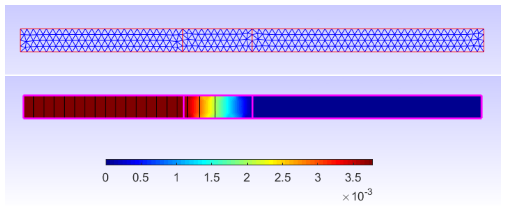
These equations present a closed-form formula for the quantities of interest $B_c$ and W. On the other hand, an FEA of the device was conducted by solving the Maxwell equations in the magnetostatics. The discrete solution is shown in Figure 2. First-order shape functions were chosen to approximate the $\phi$-component of vector potential $A_{\phi }$. The exact solution of the problem is a rational function, since the magnetic flux density $B\left(r\right)=\frac{1}{r}\frac{\partial r{A}_{\phi }}{\partial r}$ is of the first order (see Equations (1) and (2)). Consequently, the finite element model cannot fit perfectly the exact solution, and it will lead to numerical errors.

A comparison of the quantities computed with the analytic and FEA was conducted, and the relative errors are then shown in

Table 1. Comparison of analytic and FEA quantities.

	${\mathit{B}}_{\mathit{c}}$	W
Analytic	$3.757\mathrm{mT}$	$4.5239\mathrm{J}/\mathrm{m}$
FEA	$3.592\mathrm{mT}$	$4.5225\mathrm{J}/\mathrm{m}$
Rel. error	4.39	0.03

. We noticed that we had fewer errors for energy than for $B_c$. Generally speaking, FEA led to fewer errors for global quantities such as energy and higher errors for local quantities.

This illustrative example served as a simple benchmark for computing the gradient of the quantities of interest with respect to the variables R, d, and J. The next section shows some approaches that are often considered for conducting this task.

3. How Do We Compute the Gradient?

Most efficient descent methods require the gradients of the objective function and the constraints, and some approximation methods for sensitivity analysis and uncertainty propagation also rely on this gradient information. The gradient calculation is not straightforward when the functions to be derived are not explicitly expressed in terms of the variables, and this is the case for example with FEA. One method that can be easily implemented to compute the gradient is the finite-difference by imposing a small perturbation on the variables, but this presents some shortcomings, namely in precision and computational cost.

We denote the partial derivative of a function h with respect to a variable x as ${\partial }_{x}h$. In the same manner, the total derivative is written as $d_{x}h$.

3.1. Finite-Difference

The finite-difference method enabled us to approximate the gradient by imposing a small perturbation on the considered variable. For example, the derivative of the energy with respect to the variable R can be approximated using a first-order scheme as follows:

$${\partial }_{R}W\approx \frac{W(R+\epsilon ,d,J)-W(R,d,J)}{\epsilon },$$

(6)

where $\epsilon$ is a small value; this scheme implies running an additional FEA with the new value $R+\epsilon$; generally speaking, we need as many simulations as there are variables. In our example, since we had three variables ($R,d,J$), we needed three additional FEAs for computing the gradient.

The formula in (6) is called the forward difference (FD); one could also use the backward difference (BD) or centered difference (CD). The latter requires twice as many FEAs as the number of variables, but it can be more accurate (second-order approximation) than the forward and backward difference.

The choice of $\epsilon$ can be delicate, and some tuning is always necessary. In the literature, the estimation of the optimal values of $\epsilon$ is greatly studied [10,11]. Some prior knowledge of the model, such as an estimation of the second derivative, is often necessary for estimating a good value for $\epsilon$.

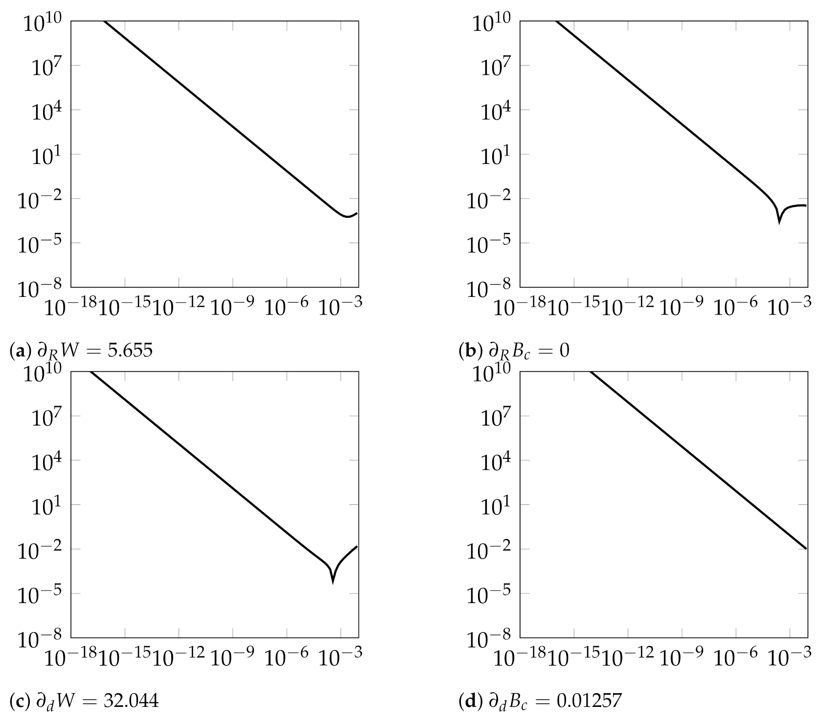
Figure 3 shows the relative error of the derivative computed with the finite-difference compared to the exact derivative, while varying $\epsilon$ from ${10}^{-18}$ to ${10}^{-2}$. We can see clearly that the derivatives depends on the value of $\epsilon$. Small values lead to more errors because of rounding errors. Moreover, high values can lead to some truncation errors, as seen for ${\partial }_{J}W$ and ${\partial }_{d}W$.

Rounding errors are caused by the accumulation of machine precision errors when using small values of $\epsilon$, while truncation errors are related to the approximation used in Equation (6); truncation errors are related to the Taylor expansion (only the first-order term is used for the approximation) and are proportional to $\epsilon$, which explains why the error for ${\partial }_{J}W$ and ${\partial }_{d}W$ increases when $\epsilon$ is big.

We can see that high values of $\epsilon$ ($>{10}^{-5}$) led to reasonably acceptable results for all the derivatives in our simple example. Nevertheless, it remains risky to use such a scheme, since the optimal value of $\epsilon$ depends on the quantity computed (global or local) and the variables for which the derivatives are calculated.

Another behavior that is seen in Figure 3 is the erratic variation when dealing with geometric variables, R and d; the chaotic discontinuities are related to the change of the mesh when varying $\epsilon$. In fact, when we apply the finite-difference scheme, we have to calculate two values of the quantity of interest for two geometries (for example, Geometry 1 with R and Geometry 2 with $R+\epsilon$). The brute approach to obtaining the two FE solutions involves re-meshing the two geometries and then solving the FE problem. This approach often leads to a “discontinuity” between the two FE solutions, which are not then approximated in the same space. In Figure 4, we see that the same geometry could be meshed differently depending on the meshing algorithm configuration. Even small variations in the geometry can lead to a change in the resulting mesh (re-meshing), which, as mentioned previously, impacts the FEA solution.

To eliminate the impact of re-meshing, one would like to keep the same mesh topology while changing the geometry, as shown in Figure 5. This approach is commonly referred to as mesh morphing.

3.2. Mesh Morphing

Different approaches for mesh morphing have been developed in order to deform an initial mesh to take into account shape modification without changing the mesh topology. The concept consists of imposing a displacement for a set of mesh nodes and determining the new coordinates for all other ones by an interpolation approach. In this context, the spring analogy [12,13], Laplacian smoothing [14], linear elasticity [15], and the radial basis function [16,17] interpolation methods are largely treated in the literature. Explaining the ideas behind each method is out of the scope of this paper; we limited ourselves to the application of the concept to our simple electromagnetic device.

Changing the geometry of an electromagnetic device by mesh morphing stands for moving the mesh nodes according to the change in the geometry. In our example, when changing the parameter R, we proceeded by moving all the mesh nodes on the boundary of the coil by $\epsilon$ in the r-direction, while all the remaining nodes stood still.

In Figure 6, we show the resulting relative error in the derivative computation when using the mesh morphing. We can see that the erratic behavior seen in Figure 3 disappeared. Mesh morphing gives a more reliable piece of information about the derivatives when compared to the one given with re-meshing, since it is less sensitive to the value of $\epsilon$. Still, it requires further attention to the choice of the best values of $\epsilon$. Moreover, carrying out a mesh morphing is not necessarily evident for 3D geometries, especially in areas where the mesh is fine such as the air gap of an electrical machine.

3.3. Discussion

We show in this section how to compute the gradient of a quantity of interest using the finite-difference method. The finite-difference has three shortcomings:

1.

The choice of the step size $\epsilon$ is not straightforward [18];

2.

Re-meshing error can highly deteriorate the information about the derivatives, and morphing an existing mesh is not straightforward for most of the geometries;

3.

The computational cost is proportional to the number of variables, which can be disadvantageous when dealing with computer-expensive simulation such as FEA.

To tackle all these issues, some researchers have proposed to use the adjoint variable method for computing the gradient from the mathematical model of the electromagnetic phenomena [6,7,19]. This approach requires an intrusive manipulation of the FE code to calculate the gradient efficiently and accurately.

The adjoint variable method is used in many fields that involve solving a large system of algebraic equations. The solution to such a system is computationally expensive; thus, computing quantities of interest involving this system is also computationally expensive. The adjoint variable method can compute the gradient with a cost less than or equal to the cost of solving the initial system. This last property makes the approach very attractive when dealing with many variables in the context of an FEA.

4. Adjoint Variable Method

The following section describes how the adjoint variable method can be implemented in a magnetostatic FEA code. The implementation can be extended to solve any other electromagnetic formulation derived from the Maxwell equations. However, an explanatory example is treated first to simplify the derivation of the adjoint equations.

4.1. Explanatory Example

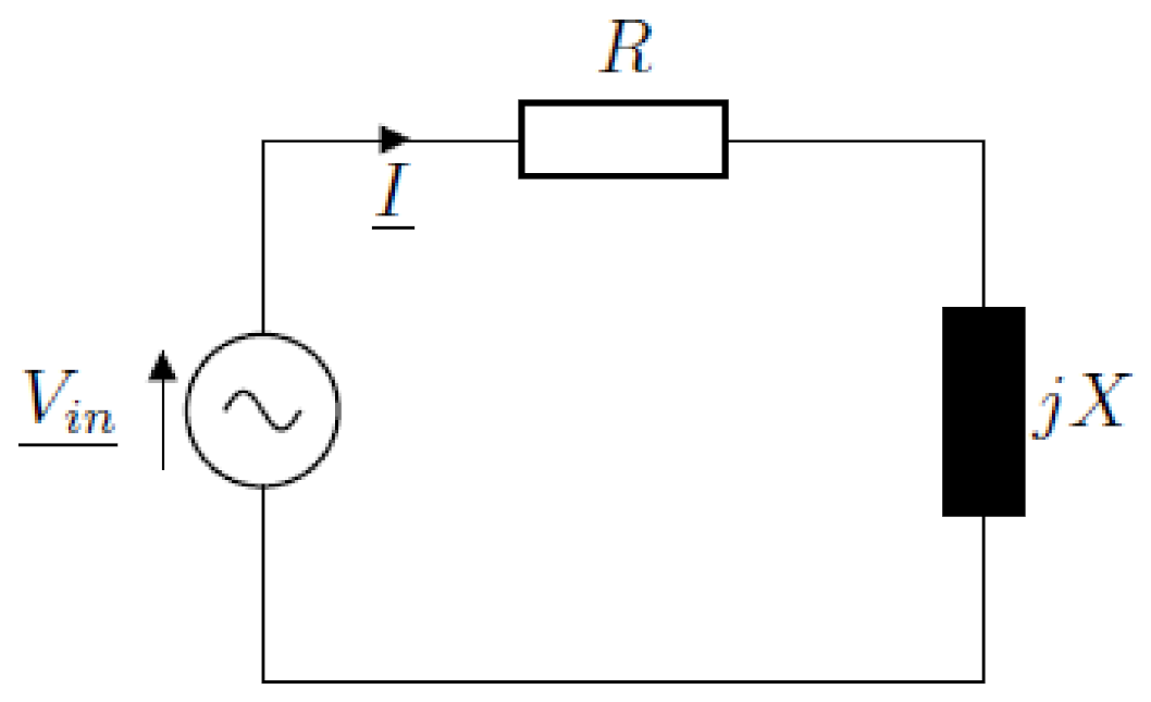
Let us consider a basic electrical circuit to explain the fundamental ideas of the adjoint variable method. Figure 7 shows an RL circuit composed of a resistor of resistance R and an inductor of reactance X driven by the sine wave voltage source $\underline{V_{in}}$.

For this circuit, we wanted to compute the Joule losses in the resistor. However, to be able to obtain this, the current flowing through the circuit has to be computed since the Joule losses are equal to the resistance times the current squared. To express the equations, we adopted the complex notation for the calculation.

The equation of the circuit is written as:

$$(R+jX)\underline{I}=\underline{V_{in}},$$

(7)

where j represents the imaginary unit ($j^2=-1$).

We supposed that the voltage source has only a real component ($\underline{V_{in}}=v_r$), and the current is written as $\underline{I}=i_r+j{i}_i$.

Therefore, Equation (7) becomes:

$$\begin{array}{cc}\hfill R{i}_r-X{i}_i& =v_r\hfill \end{array}$$

(8)

$$\begin{array}{cc}\hfill R{i}_i+X{i}_r& =0.\hfill \end{array}$$

(9)

In a more compact matrix form, we write:

$$\mathbf{K}\mathbf{u}=\mathbf{b},$$

(10)

where $\mathbf{K}=\left[\begin{array}{cc}R& -X\\ X& R\end{array}\right]$, $\mathbf{u}=\left[\begin{array}{c}{i}_r\\ i_i\end{array}\right]$, and $\mathbf{b}=\left[\begin{array}{c}{v}_r\\ 0\end{array}\right]$.

This system of equation has to be solved to identify $\mathbf{u}$, i.e., the values of the current components, and then, the Joule losses are computed by:

$$P_j=R(i_r^2+i_i^2)=R{\mathbf{u}}^{\top }\mathbf{u}.$$

(11)

Thus, we could consider R and X as the input variables of the model and an output $Pj$, as shown in Figure 8. We denote this model as:

$$f\left(\mathbf{p}\right)=\tilde{f}(\mathbf{p},\mathbf{u})=P_j,$$

(12)

where $p=(R,X)$. f and $\tilde{f}$ are different, since the first one includes $\mathbf{u}$ implicitly in its definition, while $\tilde{f}$ considers $\mathbf{u}$ as an independent variable from $\mathbf{p}$. Practically, f is the quantity of interest when looking from outside the box, while $\tilde{f}$ is only seen inside the box.

For the sake of simplification, we show the derivation of the gradient of the quantity of interest using this example, and interestingly, this derivation extends to FEA.

4.2. Derivation of Gradient

We wanted to compute the gradient of the function f, that is the partial derivatives of the function $\nabla f=\left({\partial }_{R}f,{\partial }_{X}f\right)$.

The Equation (13) expresses the relation between f and $\tilde{f}$:

$${\partial }_{\mathbf{p}}f=d_{\mathbf{p}}\tilde{f}={\partial }_{\mathbf{p}}\tilde{f}+{\partial }_{\mathbf{u}}\tilde{f}{d}_{\mathbf{p}}\mathbf{u}.$$

(13)

The quantity ${\partial }_{\mathbf{p}}\tilde{f}$ shows the explicit dependence of the function $\tilde{f}$ on the variable $\mathbf{p}$, while ${\partial }_{\mathbf{u}}\tilde{f}{d}_{\mathbf{p}}\mathbf{u}$ shows the implicit dependence of $\mathbf{p}$ through the variable $\mathbf{u}$.

To compute the gradient of the function f, we need to compute the total derivatives of $\tilde{f}$, i.e., $d_{\mathbf{p}}\tilde{f}$. In the following derivation, we only consider $\tilde{f}$, not f.

In order to express the dependence of $\mathbf{u}$ on the variable $\mathbf{p}$, we rewrite Equation (10) as:

$$g\left(\mathbf{p}\right)=\tilde{g}(\mathbf{p},\mathbf{u})=\mathbf{K}\mathbf{u}-\mathbf{b}=0.$$

(14)

Thus, the last term $d_{\mathbf{p}}\mathbf{u}$ of (13) is computed by deriving this equation:

$$d_{\mathbf{p}}\tilde{g}={\partial }_{\mathbf{p}}\tilde{g}+{\partial }_{\mathbf{u}}\tilde{g}{d}_{\mathbf{p}}\mathbf{u}=0.$$

(15)

Then, $d_{\mathbf{p}}\mathbf{u}$ is the solution of the equation:

$$d_{\mathbf{p}}\mathbf{u}=-{\left({\partial }_{\mathbf{u}}\tilde{g}\right)}^{-1}{\partial }_{\mathbf{p}}\tilde{g}.$$

(16)

By replacing $d_{\mathbf{p}}\mathbf{u}$ in (13), we obtain:

$$d_{\mathbf{p}}\tilde{f}={\partial }_{\mathbf{p}}\tilde{f}-{\partial }_{\mathbf{u}}\tilde{f}\left[{\left({\partial }_{\mathbf{u}}\tilde{g}\right)}^{-1}{\partial }_{\mathbf{p}}\tilde{g}\right].$$

(17)

This formula enables fully determining the gradient of the function f versus partial derivatives of the function $\tilde{f}$ and the equation $\tilde{g}$. However, to compute the gradient, we needed to solve the system of equations between brackets. This system involves the quantity ${\partial }_{\mathbf{p}}\tilde{g}$, which depends on the design variables $\mathbf{p}$. Thus, this system needs to be solved for each parameter, which significantly increases the computational cost.

The adjoint variable method reduces this cost by solving only one system of equations, then re-using the result for all the variables, as shown in the following equations.

By inverting the order of multiplication of the terms in (17), we obtain:

$${\partial }_{\mathbf{p}}f={\partial }_{\mathbf{p}}\tilde{f}-\left[{\partial }_{\mathbf{u}}\tilde{f}{\left({\partial }_{\mathbf{u}}\tilde{g}\right)}^{-1}\right]{\partial }_{\mathbf{p}}\tilde{g}.$$

(18)

The expression between the brackets does not depend on the parameters $\mathbf{p}$; it depends only on the solution $\mathbf{u}$ of the equation $\tilde{g}(\mathbf{p},\mathbf{u})=0$. Thus, this operation can be performed once and be applied to all the variables $\mathbf{p}$. We introduce:

$$\lambda =-{\partial }_{\mathbf{u}}\tilde{f}{\left({\partial }_{\mathbf{u}}\tilde{g}\right)}^{-1},$$

(19)

where $\lambda$ is called the adjoint variable. Then, Equation (18) becomes:

$${\partial }_{\mathbf{p}}f={\partial }_{\mathbf{p}}\tilde{f}+\lambda {\partial }_{\mathbf{p}}\tilde{g}.$$

(20)

To summarize, for computing the gradient of a function f, the following steps have to be conducted:

1.

Compute the partial derivatives for $\mathbf{u}$: ${\partial }_{\mathbf{u}}\tilde{f}$ and ${\partial }_{\mathbf{u}}\tilde{g}$;

2.

Solve the linear system: $\lambda {\partial }_{\mathbf{u}}\tilde{g}=-{\partial }_{\mathbf{u}}\tilde{f}$ for $\lambda$;

3.

Compute the partial derivatives for $\mathbf{p}$: ${\partial }_{\mathbf{p}}\tilde{f}$ and ${\partial }_{\mathbf{p}}\tilde{g}$;

4.

Calculate the adjoint using (20).

Step 1 is relatively easy to conduct. In fact, the function f is calculated from the solution $\mathbf{u}$ of the equation $g\left(\mathbf{u}\right)=0$; thus, its derivative should be no more complex than calculating the function itself. On the other hand, the partial derivative of $\tilde{g}$ with respect to $\mathbf{u}$ is sometimes already provided by the original model. If the equation $g\left(\mathbf{u}\right)=0$ is a linear system of equations, then its derivative is equal to the matrix of this system. Otherwise, if the equations $g\left(\mathbf{u}\right)=0$ are nonlinear, ${\partial }_{\mathbf{u}}\tilde{g}={\partial }_{\mathbf{u}}g$ is usually computed to solve the equation using an iterative process, e.g., Newton–Raphson, then the derivative is the Jacobian, which is often available or at least easy to determine.

Step 2 is the most computationally expensive, since it requires solving a system of linear equations of the same size as the system of equations defined by $g\left(\mathbf{u}\right)=0$. It is worth noting that even if $g\left(\mathbf{u}\right)=0$ is a nonlinear system of equations, the problem to solve in Step 2 is linear. Therefore, solving this system will always be less expensive than solving $g\left(\mathbf{u}\right)=0$; that is to say, the cost of computing the gradient will be equivalent to or less than solving $g\left(\mathbf{u}\right)=0$ for any number of variables. This property makes the adjoint variable method very attractive when dealing with many variables.

Step 3 requires the calculation of the partial derivatives of $\tilde{f}$ and $\tilde{g}$ with respect to $\mathbf{p}$. ${\partial }_{\mathbf{p}}\tilde{f}$’s calculation is performed as for ${\partial }_{\mathbf{u}}\tilde{f}$. Nevertheless, ${\partial }_{\mathbf{p}}\tilde{g}$ may not be straightforward since it involves the derivatives of the system of equations. Sometimes, this link between the variables is not as obvious as it was in our example.

Step 4 is straightforward since the total derivatives are given by Equation (20) and calculated from the product of terms determined in the previous steps.

4.3. Quantities’ Computation for the Explanatory Example

For the example above $\tilde{f}(\mathbf{p}=(R,X),\mathbf{u})=R{\mathbf{u}}^{\top }\mathbf{u}$ and $\tilde{g}(\mathbf{p}=(R,X),\mathbf{u})=\mathbf{K}\mathbf{u}-\mathbf{b}$, the quantities forming the gradient are written as:

$$\begin{array}{cc}\hfill {\partial }_{\mathbf{u}}\tilde{f}& =2R{\mathbf{u}}^{\top }\hfill \end{array}$$

(21)

$$\begin{array}{cc}\hfill {\partial }_R\tilde{f}& ={\mathbf{u}}^{\top }\mathbf{u}\hfill \end{array}$$

(22)

$$\begin{array}{cc}\hfill {\partial }_X\tilde{f}& =0\hfill \end{array}$$

(23)

$$\begin{array}{cccc}\hfill {\partial }_{\mathbf{u}}\tilde{g}& =\mathbf{K}\hfill & \hfill =& \left[\begin{array}{cc}R& -X\\ X& R\end{array}\right]\hfill \end{array}$$

(24)

$$\begin{array}{cccc}\hfill {\partial }_R\tilde{g}& ={\partial }_R\mathbf{K}\mathbf{u}\hfill & \hfill =& \left[\begin{array}{cc}1& 0\\ 0& 1\end{array}\right]\mathbf{u}\hfill \end{array}$$

(25)

$$\begin{array}{cccc}\hfill {\partial }_X\tilde{g}& ={\partial }_X\mathbf{K}\mathbf{u}\hfill & \hfill =& \left[\begin{array}{cc}0& -1\\ 1& 0\end{array}\right]\mathbf{u}.\hfill \end{array}$$

(26)

Using the expression in Equation (20), the derivative can be written as:

$$\begin{array}{cccc}\hfill d_R\tilde{f}& ={\mathbf{u}}^{\top }\mathbf{u}\hfill & \hfill +& \lambda \left[\begin{array}{cc}1& 0\\ 0& 1\end{array}\right]\mathbf{u}\hfill \end{array}$$

(27)

$$\begin{array}{cccc}\hfill d_X\tilde{f}& =\hfill & & \lambda \left[\begin{array}{cc}0& -1\\ 1& 0\end{array}\right]\mathbf{u},\hfill \end{array}$$

(28)

where $\lambda$ is obtained by solving the following linear system:

$${\mathbf{K}}^{\top }{\lambda }^{\top }=-2R\mathbf{u}.$$

(29)

We can notice that we have a general formula to compute the derivative for any value of R and X. Solving the equations is the most expensive operation. The adjoint variable method enables tackling this drawback by solving the equations only once.

4.4. Quantities Computation for FEM

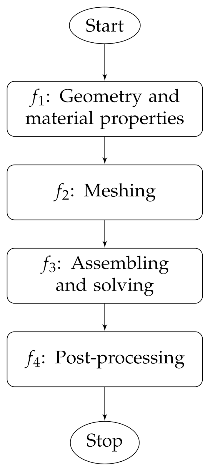
The general structure of any finite element code is presented in Figure 9. At first, the device’s geometry should be created, and the material properties are assigned to their corresponding parts. Then, a triangulation technique is used to subdivide the domains into small elements. Afterward, the mathematical model is applied to each of these small elements. The latter are then assembled into a global system of equations. This system is solved to compute the quantities of interest.

Figure 9 can be seen as multiphasic process that can be written as:

$$f\left(\mathbf{p}\right)=f_4\left(f_3\left(f_2\left(f_1\left(\mathbf{p}\right)\right)\right)\right).$$

(30)

And

$$\begin{array}{cc}\hfill G,M& =f_1\left(\mathbf{p}\right)\hfill \end{array}$$

(31)

$$\begin{array}{cc}\hfill X& =f_2\left(G\right)\hfill \end{array}$$

(32)

$$\begin{array}{cc}\hfill \mathbf{u}& =f_3(X,M)\hfill \end{array}$$

(33)

$$\begin{array}{cc}\hfill f\left(\mathbf{p}\right)& =f_4\left(\mathbf{u}\right),\hfill \end{array}$$

(34)

where $\mathbf{p}$ are the design variables, G and M are the geometry and material distribution of the design space, X is the mesh, $\mathbf{u}$ are the state variables, and $f_i$ are the functions that define each step from the flowchart shown in Figure 9.

To compute the derivative of (30), we need the derivatives of functions defining each step, then combining using the chain rule as shown below.

$${\partial }_{\mathbf{p}}f={\partial }_{\mathbf{u}}{f}_4({\partial }_X{f}_3{\partial }_G{f}_2+{\partial }_M{f}_3){\partial }_{\mathbf{p}}{f}_1.$$

(35)

This derivative representation is advantageous while debugging; indeed, it enables checking, using the finite-difference, the derivatives of each phase independently before composing all the blocks.

The Maxwell equations were solved using FEM, and the derivation went through solving a discrete system of equations. This step corresponds to the function $f_3$ in the process shown before. The system reads as follows:

$$\begin{array}{cc}\hfill \mathrm{Find}\mathbf{u}:& \mathbf{K}\mathbf{u}=\mathbf{b},\hfill \end{array}$$

(36)

where $\mathbf{K}$ is a sparse matrix, $\mathbf{u}$ is the state variable, and $\mathbf{b}$ is the source term.

Additionally, we considered a quantity of interest $f\left(\mathbf{p}\right)$ for which we wanted to compute the gradient. As for the electrical circuit, we defined two functions $\tilde{f}$ and $\tilde{g}$ for FEA:

$$\begin{array}{cc}\hfill \tilde{g}(\mathbf{p},\mathbf{u})& =\mathbf{K}(\mathbf{p},\mathbf{u})\mathbf{u}-\mathbf{b}\left(\mathbf{p}\right)=0\hfill \end{array}$$

(37)

$$\begin{array}{cc}\hfill f\left(\mathbf{p}\right)& =\tilde{f}(\mathbf{p},\mathbf{u}).\hfill \end{array}$$

(38)

This representation of the problem simplified the derivation of the gradient using the adjoint variable method as for the electrical circuit; thus, we write:

$${\partial }_{\mathbf{p}}f={\partial }_{\mathbf{p}}\tilde{f}+\lambda {\partial }_{\mathbf{p}}\tilde{g},$$

(39)

where $\lambda$ is the adjoint variable and is the solution of the linear system of equations:

$$\lambda {\partial }_{\mathbf{u}}\tilde{g}=-{\partial }_{\mathbf{u}}\tilde{f}.$$

(40)

The solution of the linear system Equation (40) is the most computationally expensive operation, and it is independent of the variables $\mathbf{p}$. Thus, the gradient computation cost is independent of the number of variables.

Computing the gradient using the adjoint method was reduced to compute the partial derivatives with respect to state variable $\mathbf{u}$ (${\partial }_{\mathbf{u}}\tilde{f}$, ${\partial }_{\mathbf{u}}\tilde{g}$) and those with respect to design variables $\mathbf{p}$ (${\partial }_{\mathbf{p}}\tilde{f}$, ${\partial }_{\mathbf{p}}\tilde{g}$).

4.5. Derivatives for State Variables

Derivatives with respect to the state variables are relatively simple to express. ${\partial }_{\mathbf{u}}\tilde{g}$ is generally always computed in the initial FEA code.

If there is no nonlinear ferromagnetic material:

$${\partial }_{\mathbf{u}}\tilde{g}=\mathbf{K}.$$

(41)

Otherwise, in the nonlinear case:

$${\partial }_{\mathbf{u}}\tilde{g}={\partial }_{\mathbf{u}}\left(\mathbf{K}\mathbf{u}\right).$$

(42)

For solving $\tilde{g}(\mathbf{p},\mathbf{u})=0$, the Jacobian matrix ${\partial }_{\mathbf{u}}\tilde{g}$ is necessary for a nonlinear solver such as Newton–Raphson. Thus, this quantity could be retrieved from the finite element code without any additional implementation effort.

On the other hand, ${\partial }_{\mathbf{u}}\tilde{f}$ can be computed efficiently because the function f is given by an explicit expression of the state variable $\mathbf{u}$.

For example, if the quantity of interest is the magnetic energy in the linear magnetostatic case that is written as:

$$\tilde{f}(\mathbf{p},\mathbf{u})=W=\frac{1}{2}{\mathbf{u}}^{\top }\mathbf{K}\mathbf{u},$$

(43)

then the derivative with respect to $\mathbf{u}$ is:

$$\begin{array}{cc}\hfill {\partial }_{\mathbf{u}}\tilde{f}& =\frac{1}{2}{\mathbf{u}}^{\top }\mathbf{K}+\frac{1}{2}{\mathbf{u}}^{\top }{\mathbf{K}}^{\top }\hfill \end{array}$$

(44)

$$\begin{array}{cc}\hfill & ={\mathbf{u}}^{\top }\mathbf{K}.\hfill \end{array}$$

(45)

For other quantities of interest f, ${\partial }_{\mathbf{u}}\tilde{f}$ could be derived and implemented with ease.

4.6. Derivatives for the Design Variables

The derivatives of the quantities $\tilde{f}$ and $\tilde{g}$ with respect to the design variables could be somewhat challenging due to the variety of parameters that could be considered. Often, in the literature, researchers separate between geometric variables and physical variables where the first are often referred to as shape sensitivity analysis [6] and the latter are mainly used in the context of topology optimization [20]. In this paper, we treated both types of variables.

4.6.1. Geometric Variables

Geometric variables are the ones that involve changing the geometry of the device studied. A geometric definition of the problem must be made before starting optimization and uncertainty quantification processes. The choice of variables is of paramount importance, since it is equivalent to defining the mathematical model of the problem studied. Clearly, it defines the nature, and the dimensions of the research space and possible solutions largely depend on it. The computation of the derivatives highly depends on the way the geometry is parameterized.

Parameterization

In the simplest configuration, the shape parameters can be viewed as a simple collection of points in 3D space. The analysis, in this case, consists of moving each of the points in the desired direction by a small amount and determining the effect on the function. This process is both complicated and expensive in terms of computation. Shape parameterization is an attempt to overcome these complexities and inefficiencies.

Shape parameterization is the method of identifying a set of parameters that together control the overall size and shape of the device being designed. This is performed by determining specific driving variables and reducing the number of design variables from the number of points in 3D space to the number of parameters.

Many methods of geometry parameterization exist, such as free-form deformation [21], the polynomial and spline method (NURBS) [22], iso-geometric analysis [23], and computer-aided design (CAD). From these categories, CAD seems to have certain capabilities that make it incredibly attractive to design engineers, such as efficiency, compactness, and adaptation to complex configurations. In addition, CAD-based parameterization methods allow for significant geometry changes. Another advantage of CAD is the availability of a comprehensive set of geometric features provided by commercial CAD systems. However, parameterizing a complex model remains a challenging task with current CAD systems.

In addition, they are not capable of calculating derivatives analytically. The commercial CAD systems’ computer codes are huge; differentiating an entire system with automatic differentiation tools may become a tedious task. Therefore, calculating derivatives of geometry with respect to design variables could be a challenge in commercial CAD software.

The derivative of the quantities $\tilde{f}$ and $\tilde{g}$ with respect to a geometric design variable $\mathbf{p}$ can be written as follows:

$$\begin{array}{cc}\hfill {\partial }_{\mathbf{p}}\tilde{f}& =\sum _{i=1}^N\left[{\partial }_{x_i}\tilde{f}{d}_{\mathbf{p}}{x}_i+{\partial }_{y_i}\tilde{f}{d}_{\mathbf{p}}{y}_i\right]\hfill \end{array}$$

(46)

$$\begin{array}{cc}\hfill {\partial }_{\mathbf{p}}\tilde{g}& =\sum _{i=1}^N\left[{\partial }_{x_i}\tilde{g}{d}_{\mathbf{p}}{x}_i+{\partial }_{y_i}\tilde{g}{d}_{\mathbf{p}}{y}_i\right],\hfill \end{array}$$

(47)

where $(x_i,y_i)$ for $i=1,\cdots ,N$ are the node coordinates used for the FEA; by writing the quantities in this form, we decouple the dependence of the quantities related to the FEA from the geometry definition. Furthermore, we decoupled the computation cost from the number of design variables since ${\partial }_{x_i}\tilde{f}$, ${\partial }_{y_i}\tilde{f}$, ${\partial }_{x_i}\tilde{g}$, and ${\partial }_{y_i}\tilde{g}$ are independent of $\mathbf{p}$.

These quantities can be computed analytically. ${\partial }_{x_i}\tilde{g}$ and ${\partial }_{y_i}\tilde{g}$ can be calculated from the finite element discretization of the Maxwell equations. In fact, the only quantity that depends on the mesh coordinates is the mapping from the reference element to an arbitrary element. Thus, only the derivative of the mapping is needed for the computation of the quantities.

We have:

$$\begin{array}{cc}\hfill {\partial }_{x_i}\tilde{g}& ={\partial }_{x_i}[\mathbf{K}\mathbf{u}-\mathbf{b}]\hfill \end{array}$$

(48)

$$\begin{array}{cc}\hfill {\partial }_{y_i}\tilde{g}& ={\partial }_{y_i}[\mathbf{K}\mathbf{u}-\mathbf{b}].\hfill \end{array}$$

(49)

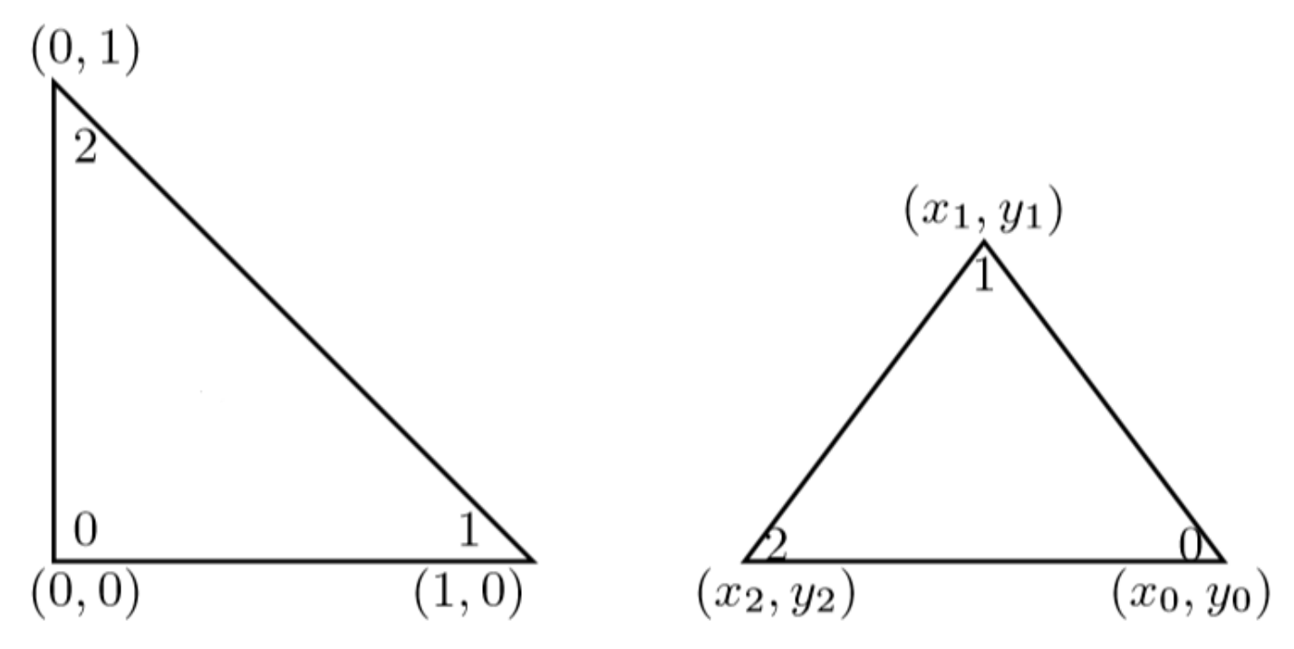
The quantities $\mathbf{K}$ and $\mathbf{b}$ are computed using the reference element concept, as shown in Figure 10.

The following equation describes how the reference element coordinates $(x_r,y_r)$ are transformed into the coordinates $(x,y)$ of an arbitrary element using the mesh nodes ($x_0$, $x_1$, $x_2$, $y_0$, $y_1$, $y_2$) defining this element:

$$(x,y)=(x_0,y_0)+(x_r,y_r){\mathbf{J}}_T,$$

(50)

with:

$${\mathbf{J}}_T=\left(\begin{array}{cc}{x}_1-x_0& y_1-y_0\\ x_2-x_0& y_2-y_0\end{array}\right).$$

The derivative of the mapping with respect to $x_0$, $x_1$, $x_2$, $y_0$, $y_1$, and $y_2$ is easy to compute; hence, ${\partial }_{x_i}\tilde{g}$ and ${\partial }_{y_i}\tilde{g}$ can be assembled as for $\tilde{g}$.

Now, let us go up to the other part of Equations (46) and (): $d_{\mathbf{p}}{x}_i$ and $d_{\mathbf{p}}{y}_i$. These quantities somewhat link the variation in the node coordinates versus the change in geometry. Hence, they represent the real link to the CAD model after the latter has been meshed. In this paper, we show how to compute these quantities without intrusive manipulation, neither in the CAD software nor in the mesh tool.

Geometric parameters are related to one or many edges that separate different regions (faces), as shown in Figure 11. This numbering is very useful for FEA since it enables imposing external conditions. For example, we used $E2$ to impose a Dirichlet boundary condition, and the face $F3$ was used for imposing a current density J.

We used this numbering for calculating the desired quantities. In this example, we have two geometric design variables R and d, as shown in Figure 11. These variables enable the positioning and sizing of the coil modeled by the face $F3$; thus, they mainly act on edges surrounding the coil, namely $E3$, $E4$, $E6$, and $E9$. Hence, $d_{\mathbf{p}}{x}_i$ and $d_{\mathbf{p}}{y}_i$ are computed only for the mesh nodes that lie on these edges and not on all the other nodes. Therefore, we write:

$$\begin{array}{cc}\hfill d_{\mathbf{p}}{x}_i& =\left\{\begin{array}{cc}{d}_{\mathbf{p}}{x}_i,\hfill & \mathrm{if}\mathrm{node}i\mathrm{is}\mathrm{on}E3,E4,E6\mathrm{or}E9.\hfill \\ 0,\hfill & \mathrm{otherwise}.\hfill \end{array}\right.\hfill \end{array}$$

(51)

$$\begin{array}{cc}\hfill d_{\mathbf{p}}{y}_i& =\left\{\begin{array}{cc}{d}_{\mathbf{p}}{y}_i,\hfill & \mathrm{if}\mathrm{node}i\mathrm{is}\mathrm{on}E3,E4,E6\mathrm{or}E9.\hfill \\ 0,\hfill & \mathrm{otherwise}.\hfill \end{array}\right.\hfill \end{array}$$

(52)

The edges $E3$, $E4$, $E6$, and $E9$ define a rectangle. The objective is to define the rectangle contour using a parametric equation as follows:

$$P\left(t\right)=\left(x\right(t),y(t\left)\right).$$

(53)

In general, one could propose many ways to parameterize a shape. For the rectangle, we could parameterize each edge independently and compute the derivative or use a single parametrization for the whole rectangle as below:

$${\displaystyle x\left(t\right)=R+\frac{d}{2}\left[1+\mathrm{sign}\left(\cos \right(t\left)\right)\right]}$$

$$y\left(t\right)=\frac{h}{2}\left[1+\mathrm{sign}\left(\sin \right(t\left)\right)\right],$$

and $t\in [0,2\pi [$.

The derivatives of $x\left(t\right)$ and $y\left(t\right)$ with respect to the design variables are computed with ease:

$$\begin{array}{cc}\hfill d_{R}x& =1\hfill \end{array}$$

(54)

$$\begin{array}{cc}\hfill d_{R}y& =0\hfill \end{array}$$

(55)

$$\begin{array}{cc}\hfill d_{d}x& =\frac{1}{2}\left[1+\mathrm{sign}\left(\cos \right(t\left)\right)\right]=\frac{x-R}{d}\hfill \end{array}$$

(56)

$$\begin{array}{cc}\hfill d_{d}y& =0.\hfill \end{array}$$

(57)

Equations (54)–() were evaluated using the node coordinates previously identified, then were used in Equations (46) and () to compute ${\partial }_{\mathbf{p}}\tilde{f}$ and ${\partial }_{\mathbf{p}}\tilde{g}$.

Now, we have everything for the computation of the gradient of a quantity of interest with respect to geometry variables using the adjoint variable method.

In this section, we computed the shape sensitivities $d_{\mathbf{p}}{x}_i$ and $d_{\mathbf{p}}{y}_i$ for a rectangular shape using a parametric equation. This framework is extendable to different types of geometry and design variables. In Appendix A, we derive the shape sensitivities for some recurrent types of geometries.

4.6.2. Physical Variable

The physical variables that can be considered in electromagnetic modeling are the permeability of ferromagnetic materials, the coercive field of magnets, and the imposed current density. This kind of modeling is commonly used in the context of topology optimization, where the objective, in general, is to reduce the volume of material present in a device. Topology optimization was first introduced in the context of structural optimization before being extended to other physical fields such as heat transfer, fluid dynamics, and electromagnetism.

In this paper, the objective was to derive the formula that enables computing the gradient for parameters that act on the physical properties of electromagnetic devices.

Permeability

If a parameter $\mathbf{p}$ controls how the permeability $\mu$ varies, the derivatives ${\partial }_{\mathbf{p}}\tilde{f}$, ${\partial }_{\mathbf{p}}\tilde{g}$ can be computed:

$$\begin{array}{c}\hfill {\partial }_{\mathbf{p}}\tilde{g}={\partial }_{\mathbf{p}}\left[\mathbf{K}\mathbf{u}-\mathbf{b}\right]={\partial }_{\mu }\left[\mathbf{K}\mathbf{u}\right]d_{\mathbf{p}}\mu .\end{array}$$

(58)

The quantity $d_{\mathbf{p}}\mu$ highlights the sensitivity of $\mu$ with respect to the design variable $\mathbf{p}$.

In the literature, we can find multiple ways of modeling. For example, the density method uses a polynomial mapping for the parameterization [24].

$$\mu ={\mu }_{air}+({\mu }_{iron}-{\mu }_{air}){\mathbf{p}}^n,$$

(59)

with ${\mu }_{air}$ and ${\mu }_{iron}$ respectively the air and iron permeabilities. This method enabled us to choose where in the studied domain to put iron or air. In this case, ${\partial }_{\mathbf{p}}\mu$ is written as:

$$d_{\mathbf{p}}\mu =n({\mu }_{iron}-{\mu }_{air}){\mathbf{p}}^{n-1}.$$

(60)

Coercive Field

As for the permeability, if $\mathbf{p}$ controls the magnetization $\mathbf{M}$ of a permanent magnet, one could, similarly, deduce the derivatives:

$$\begin{array}{c}\hfill {\partial }_{\mathbf{p}}\tilde{g}={\partial }_{\mathbf{p}}\left[\mathbf{K}\mathbf{u}-\mathbf{b}\right]=-{\partial }_{\mathbf{M}}\mathbf{b}{d}_{\mathbf{p}}\mathbf{M}.\end{array}$$

(61)

The quantity $d_{\mathbf{p}}\mathbf{M}$ was computed based on the design variable; $\mathbf{p}$ can be the magnitude, the direction of the coercive field, etc.

Imposed Current Density

Following the same principle, the derivative with respect to a variable that controls the current density J is:

$$\begin{array}{c}\hfill {\partial }_{\mathbf{p}}\tilde{g}={\partial }_{\mathbf{p}}\left[\mathbf{K}\mathbf{u}-\mathbf{b}\right]=-{\partial }_J\mathbf{b}{d}_{\mathbf{p}}J.\end{array}$$

(62)

4.7. Discussion

In the previous section, we showed the derivation of the gradient of a quantity of interest from a finite element code using the adjoint variable method.

The discrete adjoint approach can be implemented in a modular fashion using the same data structures/solution strategy as the analysis, as shown in Figure 12.

To summarize, the adjoint is composed of three main steps; at the parameter setting, one should compute the sensitivities with respect to the design variables (geometric and physical), then assemble of the quantities ${\partial }_{\alpha }\tilde{f}$, ${\partial }_{\alpha }\tilde{g}$ where $\alpha \in \{\mathbf{u},x_i,y_i,\mu ,\mathbf{M},J\}$; afterwards, the adjoint problem is solved, and finally, the gradient of the quantity of interest is computed as:

$$\begin{array}{cc}\hfill \nabla f& =\left[{\partial }_{x_i}\tilde{f}+\lambda {\partial }_{x_i}\tilde{g}\right]d_{\mathbf{p}}{x}_i\hfill \\ \hfill & +\left[{\partial }_{y_i}\tilde{f}+\lambda {\partial }_{y_i}\tilde{g}\right]d_{\mathbf{p}}{y}_i\hfill \\ \hfill & +\left[{\partial }_{\mu }\tilde{f}+\lambda {\partial }_{\mu }\tilde{g}\right]d_{\mathbf{p}}\mu \hfill \\ \hfill & +\left[{\partial }_{\mathbf{M}}\tilde{f}+\lambda {\partial }_{\mathbf{M}}\tilde{g}\right]d_{\mathbf{p}}\mathbf{M}\hfill \\ \hfill & +\left[{\partial }_J\tilde{f}+\lambda {\partial }_J\tilde{g}\right]d_{\mathbf{p}}J.\hfill \end{array}$$

In this equation, one can see that all the dependencies on the design variables $\mathbf{p}$ are outside the most computationally expensive operations, namely the solution of the adjoint problem and the assembling of the different quantities. The independence of the number of design variables makes the adjoint variable method very attractive for treating problems with large numbers of design variables and few objectives.

The formulation, presented in this paper, can be applied to any problem that is formulated as a single state equation $\mathbf{Ku}=\mathbf{b}$. However, in the case of multiple state equations, multiple adjoint problems need to be solved. This can be the case in magnetodynamics where an Euler scheme is applied to decompose the time domain into multiple time steps. Then, for each step, there is a system of the form $\mathbf{Ku}=\mathbf{b}$ to solve and an equivalent adjoint system that is solved. In this case, one would need to store all the adjoints computed at each time step to be able to compute the gradient of a quantity of interest. This aspect was not considered in the present paper, but the major ideas presented in this paper can be extended to this aspect.

To show the usefulness and effectiveness of the adjoint variable method, in the next section, we treat some examples to highlight the advantages of the adjoint variable approach.

5. Examples

This section is dedicated to numerical tests of the adjoint variable method. First, we conducted two comparisons of the gradient computed using the adjoint variable to the ones computed either analytically or using the finite-difference method; this step enabled us to show the precision and the computational gain.

Then, we used the adjoint variable method in the context of optimization. For this task, we addressed two well-known benchmarks treated by electromagnetic community researchers called Testing Electromagnetic Analysis Methods (TEAM) Workshops [25,26] to perform parametric optimization and one additional test case for topology optimization [27].

To obtain an overview of the benefits obtained with the adjoint variable method, we solved these problems using two methods: the SQP algorithm from the MATLAB Optimization toolbox with the gradient of the quantities of interest that is computed using the adjoint variable method, as well as by the genetic algorithm (GA) (from the MATLAB Global Optimization toolbox [28]). To handle the local search of the SQP algorithm, we used a multi-start strategy. We ran multiple executions with different initial points; the initial points were sampled using the Latin hypercube sampling (LHS) technique to obtain a uniform distribution over the entire design space. We chose GA because of its simplicity of coupling with an FEA and its extensive use to address this type of problem.

5.1. Solenoid Model

We considered the example treated in Section 2 of the paper, where we made a comparison between the analytic and FEA computation of the quantities of interest. We conducted the same comparison on the gradient of these quantities, as shown in

Table 2. Comparison of analytic and adjoint variable gradients.

	${\mathit{B}}_{\mathit{c}}$	${\mathit{\partial }}_{\mathit{R}}{\mathit{B}}_{\mathit{c}}$	${\mathit{\partial }}_{\mathit{d}}{\mathit{B}}_{\mathit{c}}$	${\mathit{\partial }}_{\mathit{J}}{\mathit{B}}_{\mathit{c}}$	W	${\mathit{\partial }}_{\mathit{R}}\mathit{W}$	${\mathit{\partial }}_{\mathit{d}}\mathit{W}$	${\mathit{\partial }}_{\mathit{J}}\mathit{W}$
Analytic	3.757	0	0.0126	0.376	4.5239	5.655	32.044	904.78
FEA + Adjoint	3.592	0.006	0.0125	0.359	4.5225	5.655	32.032	904.50
Rel. error %	4.39	0.60	0.38	4.39	0.03	0.00	0.04	0.03

.

One can notice that the gradients of $B_c$ and W computed by the adjoint variable method correspond to the ones computed analytically with a relative error of the same magnitude as for the quantities $B_c$ and W. This check enabled us to validate the reliability of the method for the computation of the gradient. In the next section, we focus on more challenging problems with more variables and more complexity.

5.2. TEAM Workshop 22

5.2.1. Problem Statement

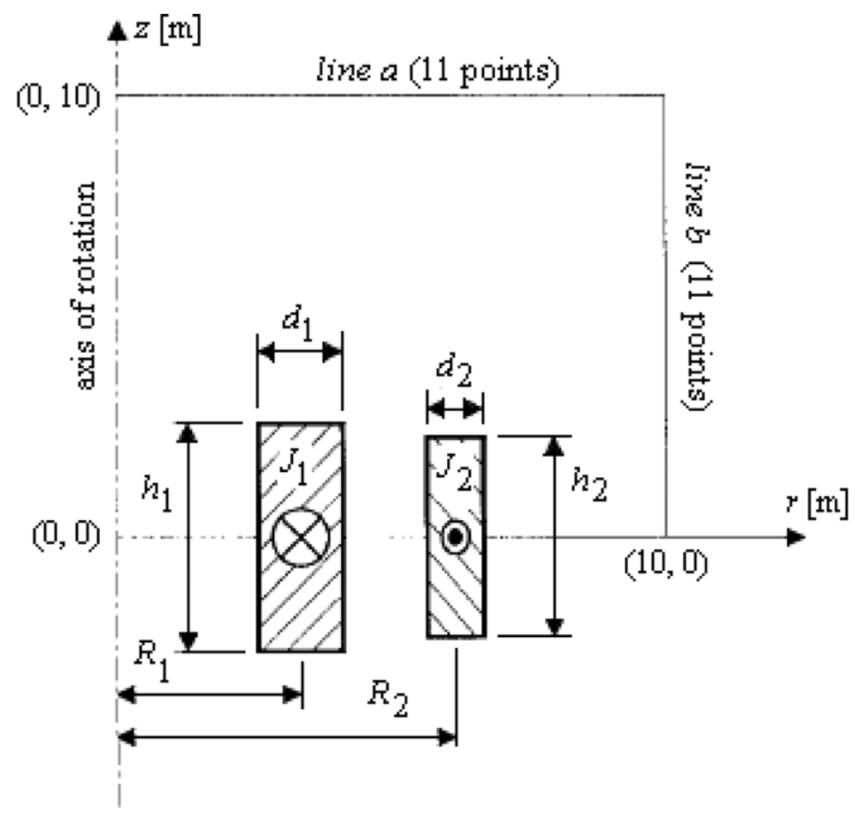
We studied a classical test case of electromagnetism: the storage of magnetic energy by two coils. The details of the device were detailed in [25], and its geometry is shown in Figure 13: one coil to store energy, the other to reduce the leakage flux. This flux was calculated along Line a and Line b.

The benchmark model was axisymmetric, so we only built one half. In this part, we discuss some aspects of the model, mainly related to the parameterization and the FEA.

Parameterization

The geometry of the device was simple; it was composed of three rectangles, as shown in Figure 14: two for the coils and one limiting the studied domain ($[0,15]\times [0,15]$), which holds the two coils.

The variables considered in the optimization problem were the ones related to the coils (position, size, current density imposed). The variables $(R_1,R_2,h_1/2,h_2/2,d_1,d_2)$ were used for the parameterization of the geometry (see Appendix A.1 for the shape sensitivities), while the current densities $(J_1,J_2)$ are physical variables that were parameterized in the FE model.

Simulation

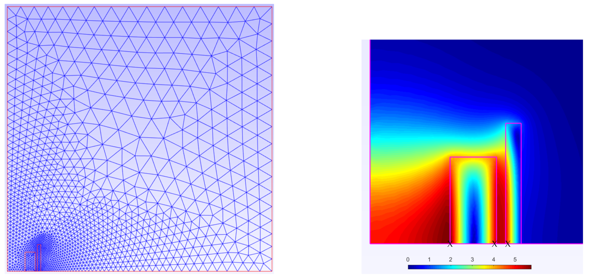
In the FEA, the geometry was meshed as shown in Figure 15 on the left. A fine mesh was imposed around the coils and a coarse one far from them. On the right of Figure 15, the distribution of the flux density around the coils is shown.

Optimization Problem

This problem is described by eight variables that must be optimized to find the design configuration that gives a given magnetic energy for a minimal leakage flux. This is formulated as:

$$\begin{array}{c}\hfill \underset{\mathbf{p}}{\min }OF\left(\mathbf{p}\right)=B_{stray}^2\left(\mathbf{p}\right)/B_{norm}^2+|E\left(\mathbf{p}\right)-E_{ref}|/E_{ref}\end{array}$$

(63a)

$$\begin{array}{c}\hfill \mathrm{s}.\mathrm{t}.(J_1-54)/6.4+\left|B(\mathbf{p},P_1)\right|\le 0\end{array}$$

(63b)

$$\begin{array}{c}\hfill (J_1-54)/6.4+\left|B(\mathbf{p},P_2)\right|\le 0\end{array}$$

(63c)

$$\begin{array}{c}\hfill (J_2-54)/6.4+\left|B(\mathbf{p},P_3)\right|\le 0\end{array}$$

(63d)

$$\begin{array}{c}\hfill 1.8\le R_1+A_2+(d_1+d_2)/2\le 5\end{array}$$

(63e)

where $E_{ref}=180MJ$, $B_{norm}=200\mathsf{\mu }T$, and $p=(R_1,A_2,h_1/2,h_2/2,d_1,d_2,J_1,J_2)$ are the design variables, and their bounds are shown in

Table 3. Bounds of the design variables for TEAM Problem 22.

p	${\mathit{R}}_1$	${\mathit{A}}_2$	${\mathit{h}}_1/2$	${\mathit{h}}_2/2$	${\mathit{d}}_1$	${\mathit{d}}_1$	${\mathit{J}}_1$	${\mathit{J}}_2$
min	1.0	0.001	0.1	0.1	0.1	0.1	10	−30
max	4.0	3.9	1.8	1.8	0.8	0.8	30	−10

.

The variable $A_2$ was introduced by replacing the variable $R_2$, which can be calculated by $R_2=R_1+A_2+(d_1+d_2)/2$. For more details about the optimization problem, the reader may refer to [29].

5.2.2. Gradient Check

The objective here was to compare the gradient computed using the finite-difference to the one computed using the adjoint variable method. To validate the effectiveness of the adjoint variable method, the approach was tested against the gradient computed using the centered finite-difference (CD) (${\partial }_{p_i}OF\left(\mathbf{p}\right)\approx \frac{OF(p_1,\cdots ,p_i+\epsilon ,\cdots )-OF(p_1,\cdots ,p_i-\epsilon ,\cdots )}{2\epsilon }$) and the mesh morphing technique or remeshing technique. The mesh morphing (MM) technique enables “small” changes of the shape while maintaining the topology (node connectivity) of the mesh. The aim of using such a technique is to reduce the errors due to re-meshing that was shown in the illustrative example treated in Section 3.

The results of the comparison are summarized in

Table 4. Gradient comparison for TEAM Workshop 22.

Method	${\mathit{\partial }}_{{\mathit{R}}_1}\mathit{OF}$	${\mathit{\partial }}_{{\mathit{R}}_2}\mathit{OF}$	${\mathit{\partial }}_{{\mathit{h}}_1/2}\mathit{OF}$	${\mathit{\partial }}_{{\mathit{h}}_2/2}\mathit{OF}$	${\mathit{\partial }}_{{\mathit{d}}_1}\mathit{OF}$	${\mathit{\partial }}_{{\mathit{d}}_2}\mathit{OF}$	${\mathit{\partial }}_{{\mathit{J}}_1}\mathit{OF}$	${\mathit{\partial }}_{{\mathit{J}}_2}\mathit{OF}$	Time (s)
CD w/o MM	36.497	−23.592	15.756	−19.098	35.757	−93.534	8.418 × 10${}^{-7}$	8.444 × 10${}^{-7}$	7.02
CD w/ MM	24.803	−19.212	13.726	−10.616	25.855	−81.817	8.418 × 10${}^{-7}$	8.444 × 10${}^{-7}$	4.06
Adjoint	24.827	−19.222	13.725	−10.619	25.852	−81.824	8.418 × 10${}^{-7}$	8.444 × 10${}^{-7}$	1.27

. It shows the gradient of the problem’s objective function in the optimum. For more details, the reader may refer [25].

For finite-difference schemes, we tried different values of $\epsilon$, ranging from ${10}^{-10}$ to ${10}^{-2}$. In the table, only the values that correspond to the best results in terms of relative error are shown.

When using mesh morphing (CD w/ MM), the gradients were coherent in less than $1\%$ error relative to the gradient computed with the adjoint, with a speedup of 3.2. This speedup was attained thanks to the main property of the adjoint variable method that solves fewer equations. However, when not using mesh morphing (CD w/o MM), which means generating a new mesh for each geometry change, re-meshing errors appeared to perturb the gradient information highly (relative error higher than 150%).

It is worth noting that the difference in time for CD w/ MM and CD w/o MM was related to the overhead of regenerating a new mesh for all geometry variations.

In general, mesh morphing is not always a simple task; in this example, it was possible to morph the mesh nodes to correspond to the geometry change thanks to the simple shapes involved in the modeled device (rectangular regions). Thus, without using mesh morphing, the finite-difference method may lead to significant errors when compared to the adjoint variable method even with fine-tuning the step size $\epsilon$. Furthermore, a speedup of $5.5$ was attained for the computation of the gradient, which confirmed the efficiency of the adjoint variable method.

5.2.3. Optimization Results

After running the optimization, the obtained results from SQP and GA are shown in

Table 5. TEAM Workshop Problem 22 optimization results.

Algorithm	SQP	GA
Individuals	100	200
$R_1$	1.336	1.457
$A_2$	0.027	0.481
$h_1/2$	1.011	1.209
$h_2/2$	1.452	1.800
$d_1$	0.677	0.347
$d_2$	0.269	0.121
$J_1$	15.579	19.834
$J_2$	−15.069	−17.305
$OF$	0.00197	0.03502
# evals	73,254	16,0201

For GA, “Individuals” indicates the population size, while for SQP, it indicates the number of multi-start runs. “# evals” indicates the number of evaluations of the finite element simulation.

.

We noticed that SQP significantly outperformed GA in terms of the quality of the solution. Indeed, 17% of the solutions obtained from different runs of SQP had an objective function value lower than 0.05 while being distinct in terms of variables; this fact justified the high multi-modality of this problem. In terms of cost, SQP assisted by the adjoint variable method was better than GA; SQP reduced the cost by more than half.

5.2.4. Discussion

For this test case, we detailed the steps to use the adjoint variable method for the parametric design of an electromagnetic device. First, we showed a comparison of the gradient for the finite-difference method. The adjoint variable method showed highly satisfactory results; it enabled speeding up the computation by more than 5.5-times. Then, we showed the result of an optimization using SQP and compared it to the performances of GA. The adjoint variable showed its effectiveness both in terms of the solution quality and computational cost.

5.3. TEAM Workshop 25

5.3.1. Problem Statement

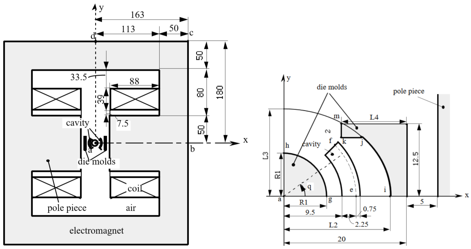
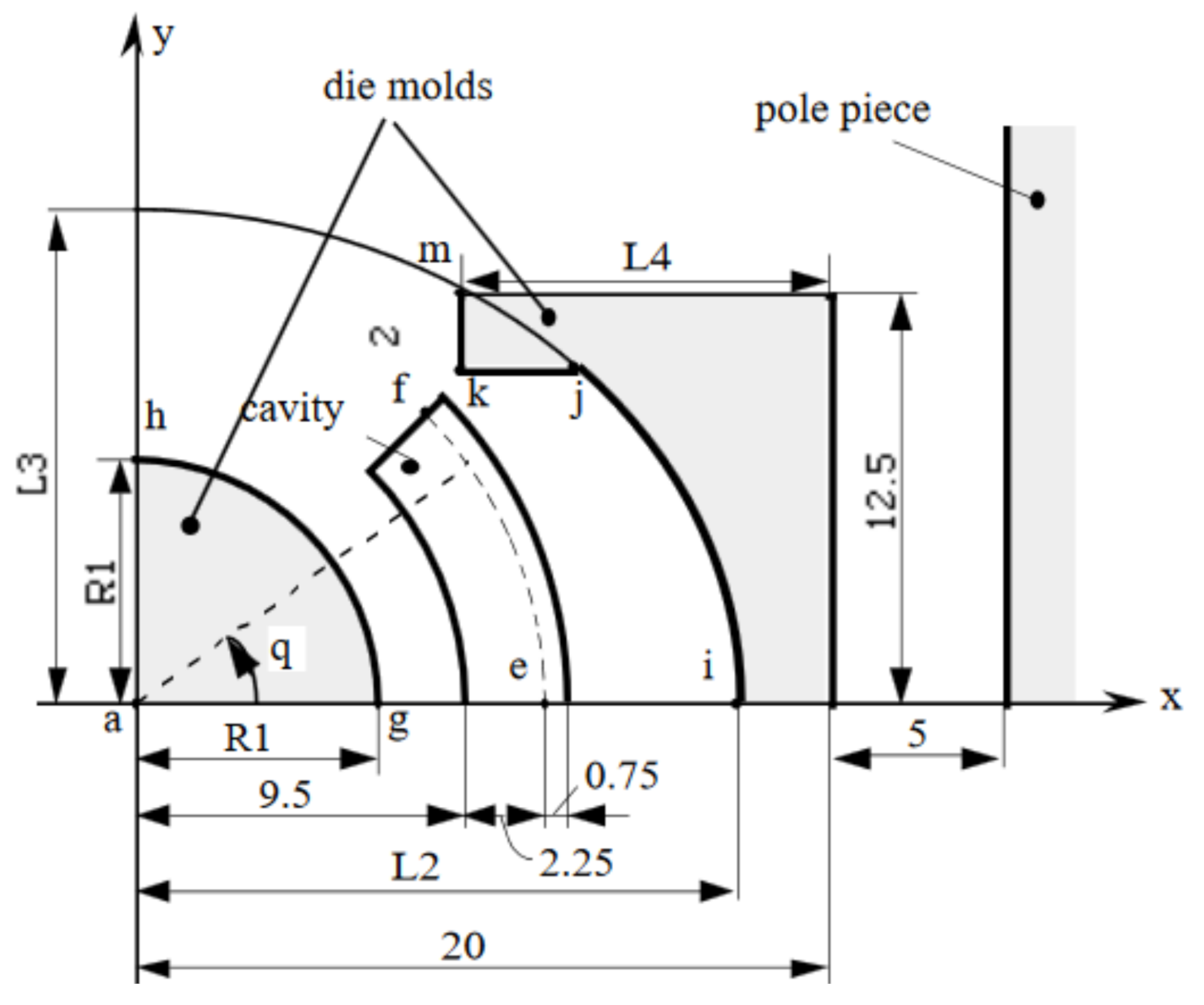
The device used in this test case was used to orient the magnetic powder and make anisotropic permanent magnets [26]. The magnetic powder was placed in the cavity. The direction and strength of the magnetic field must be controlled to obtain the required magnetization. One coil creates this magnetic field. The current density was set to $1.239219{\mathrm{A}/\mathrm{mm}}^2$. The die assembly and the electromagnet were made of nonlinear permeability steel. The geometry of the whole device is shown in Figure 16 where the dimensions are in meters.

A model of the device was created. By exploiting the symmetries, only a quarter of the device was sufficient for the FEA.

Parameterization

The geometry of the device was created and parametrized as shown in Figure 17. The geometry was composed of six regions ($F1$–$F6$). The region $F2$ was used for imposing the current density, while regions $F1$, $F4$ and $F5$ were used for the ferromagnetic material. Other regions were considered as air.

The variables considered in the optimization were related to the mold shape of the die press. The inner mold was controlled by the variable $R1$, while the outer mold was controlled by the variables $(L2,L3,L4)$. The parameterization was somewhat more challenging than the previous test case because of the elliptical shape of the outer mold (see Appendix A.2).

Simulation

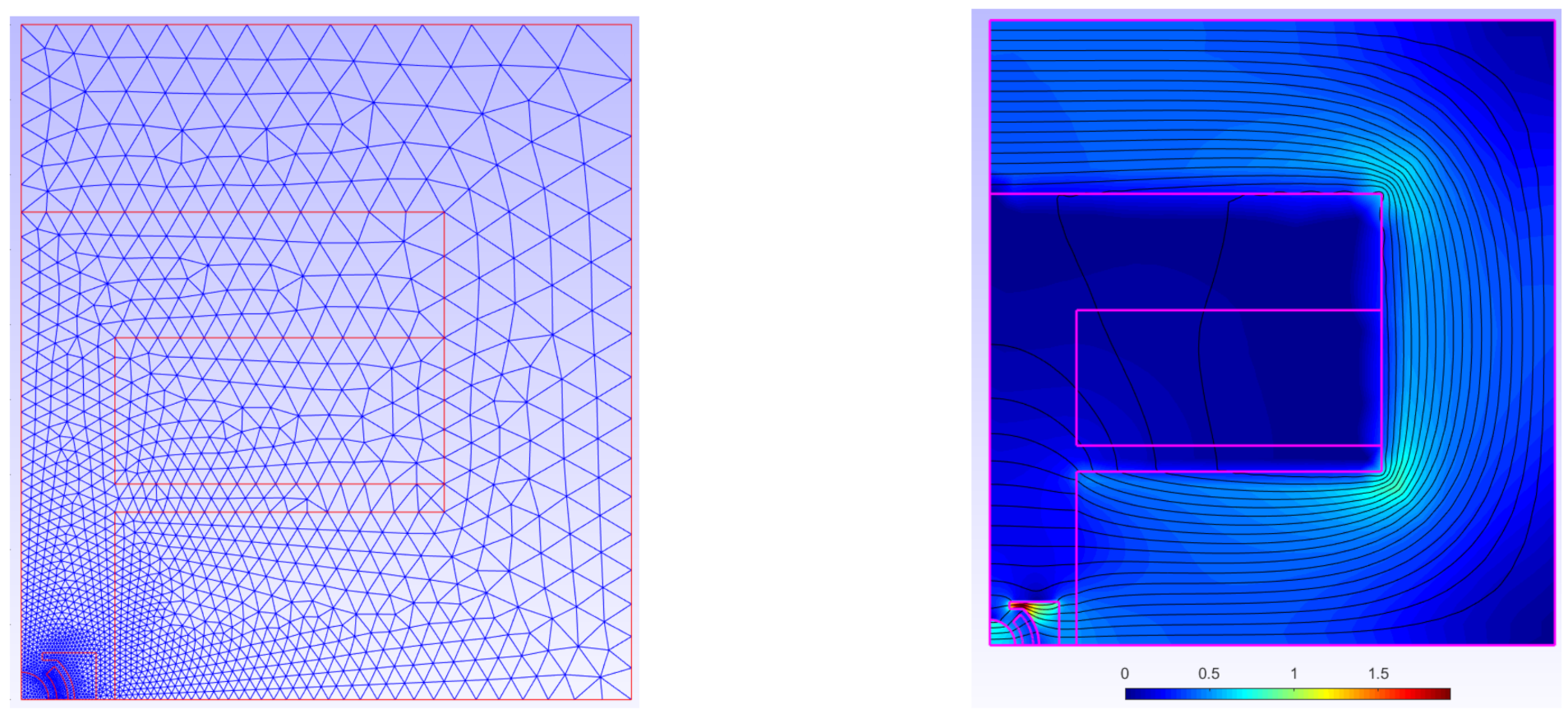
In the FEA, the geometry was meshed as shown in Figure 18 on the left. A fine mesh was imposed around the molds and a coarse mesh far from them. At the right, in the same figure, the distribution of the flux density is shown.

Optimization Problem

This optimization of shape had the objective of obtaining a radial flux density in the cavity space and of the same constant magnitude as 0.35 T. The objective function W was the squared error between the values $Bx$ and $By$ sampled at 10 positions along the arc of e–f, shown in Figure 16.

$$\underset{p}{\min }W\left(p\right)=\sum _{i=1}^{10}{(B_{xip}-B_{xio})}^2+{(B_{yip}-B_{yio})}^2$$

(64)

where $p=(R1,L2,L3,L4)$ are the design variables (their bounds are shown in

Table 6. Bounds of the design variables for TEAM Problem 25.

p	$\mathit{R}1$	$\mathit{L}2$	$\mathit{L}3$	$\mathit{L}4$
min	5.0	12.6	14	4
max	9.4	18	45	19

), $B_{xio}=0.35\cos \left(\frac{\pi }{40}i\right)$, $B_{yio}=0.35\sin \left(\frac{\pi }{40}i\right)$, and $B_{xip}$ and $B_{yip}$ were computed by the FEA of the device [29].

5.3.2. Optimization Results

The results are summarized in

Table 7. TEAM Workshop Problem 25 optimization results.

Algorithm	SQP	GA
Individuals	100	100
R1	7.31	7.51
L2	14.21	14.64
L3	14.11	14.39
L4	14.37	14.44
W	7.62 × 10${}^{-\mathbf{5}}$	12.44 × 10${}^{-5}$
# evals	954	10,100

.

The SQP gave the best results in terms of the solution quality (smaller value of W) and computational cost (smaller value of # evals).

5.3.3. Discussion

For this test case, the adjoint variable method was applied to a nonlinear problem. The method showed its superiority when compared to a conventional approach.

5.4. Electromagnet

5.4.1. Problem Statement

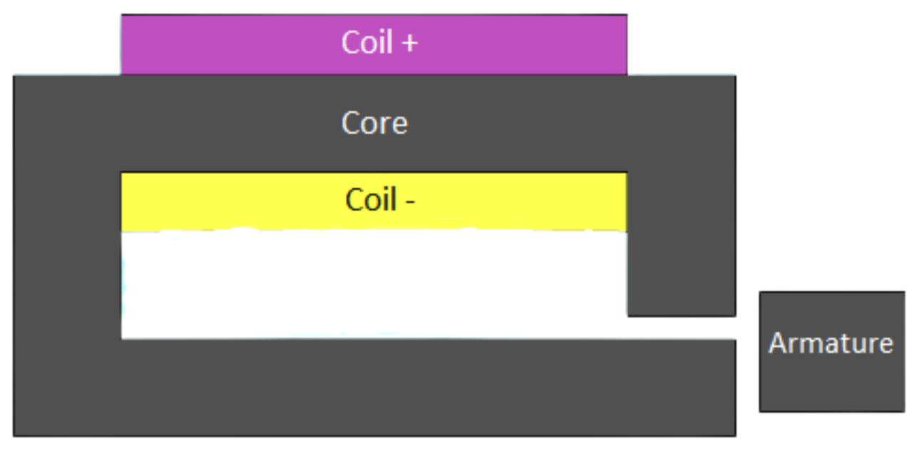
The device we deal with in this part was the electromagnet shown in Figure 19. It utilized an iron core surrounded by electrified coils to attract the armature. The armature and the core were a ferromagnetic material, and the relative magnetic permeability of the armature was 2000, while that of the core was 1000. A coil of 1A current would the core with 420 turns. The air gap between the armature and the right end of the core was fixed at 2 mm [27].

The objective here was to find the optimal shape of the core that maximized the force applied on the armature using topology optimization.

5.4.2. Topology Optimization

To carry out topology optimization in general, we needed a material distribution method, an optimization algorithm, and a numerical model.

Among the existing material distribution methods in the literature, we can count the homogenization methods, the density methods, and the boundary methods [30]. For this paper, we used the density method for its ease of application. This method consists of discretizing the domain to be optimized and using each cell as an optimization variable. Each cell takes an artificial density, which is assimilated to the presence or absence of materials at this spatial position. The link between the properties to be varied in the model and the artificial density is governed by an interpolation equation, commonly called mapping. The mappings used here were the ones from the solid isotropic material with penalization (SIMP) method [30,31].

The mapping of the relative permeability ${\mu }_r$ is written as:

$${\mu }_r=({\overline{\mu }}_r-1)p_1+1,$$

(65)

where ${\overline{\mu }}_r$ is the relative permeability of iron and $p_1$ is the density variable for iron $p_1\in [0,1]$.

The mapping of the current density J is written as:

$$J=\overline{J}(p_2-p_3),$$

(66)

where $\overline{J}>0$ is the current density imposed in copper and $p_2$, $p_3$ are the density variables for positive current density and negative current density, respectively $p_2,p_3\in [0,1]$.

It is worth noting that different mappings have been proposed in the literature. We considered this basic mapping for its simplicity, since the purpose of this paper was not to compare the different mappings, but to demonstrate the benefits of the adjoint variable method in the context of topology optimization.

Optimization Problems

The objective was to optimize the material distribution in this device to maximize the force applied by the core on the armature. Therefore, we considered two optimization problems:

1.

The mono-material problem as shown on the left of Figure 20;

• Only the right part of the core was considered for optimization;
• Only the distribution of iron was considered;

2.

The multi-material problem as shown on the right of Figure 20;

• The whole core and the coil were considered for optimization;
• In addition to iron, the distribution of copper was also considered.

The mono-material optimization problem is written as follows:

$$\begin{array}{c}\hfill \underset{\mathbf{p}}{\min }-F\left(\mathbf{p}\right)\\ \hfill \mathrm{s}.\mathrm{t}.\sum _{i=1}^{270}{p}_{1i}\le 252\\ \hfill 0\le p_{1i}\le 1,i=1,\dots ,270,\end{array}$$

(67)

where F is the force and $p_i$ are the density variables at each cell. The first constraint aimed to limit the maximum volume of iron to be less than the initial design.

On the other hand, the multi-material problem considers the distributions of iron and copper on a more significant design space. This problem is more challenging to tackle; it treats two materials (iron and copper) represented by three artificial densities, one for iron, one for positive current density, and the last for negative current density. The corresponding optimization problem is written as follows.

$$\begin{array}{c}\hfill \underset{\mathbf{p}}{\min }-F\left(\mathbf{p}\right)\\ \hfill \mathrm{s}.\mathrm{t}.\sum _{i=1}^{2100}{p}_{1i}\le 1197\\ \hfill \sum _{i=1}^{2100}{p}_{2i}\le 210\\ \hfill \sum _{i=1}^{2100}{p}_{2i}=\sum _{i=1}^{2100}{p}_{3i}\\ \hfill p_{1i}+p_{2i}+p_{3i}\le 1,i=1,\dots ,2100\\ \hfill p_{1i},p_{2i},p_{3i}\ge 0,i=1,\dots ,2100,\end{array}$$

(68)

where $p_{1i}$, $p_{2i}$, and $p_{3i}$ are the densities of iron, positive current density, and negative current density, respectively. The first two constraints limited the maximum volume of iron and copper to be less than the initial design. The third constraint imposed current conservation. The fourth constraint aimed to impose that each cell contains a single material.

5.4.3. Results and Discussion

Mono-Material Problem

To solve the optimization problem, we performed 31 optimizations using SQP and the adjoint variable method with different random initial points.

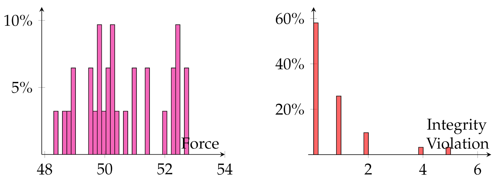
Figure 21 shows the obtained results; the histogram in the left show the distribution of the values of the force obtained from the solution of each of the 31 runs, and the histogram on the right highlights the number of variables that were neither zero nor one, but a value between the two (an intermediate material that satisfies the following formula $p(1-p)>{10}^{-4}$ where p is the density variable).

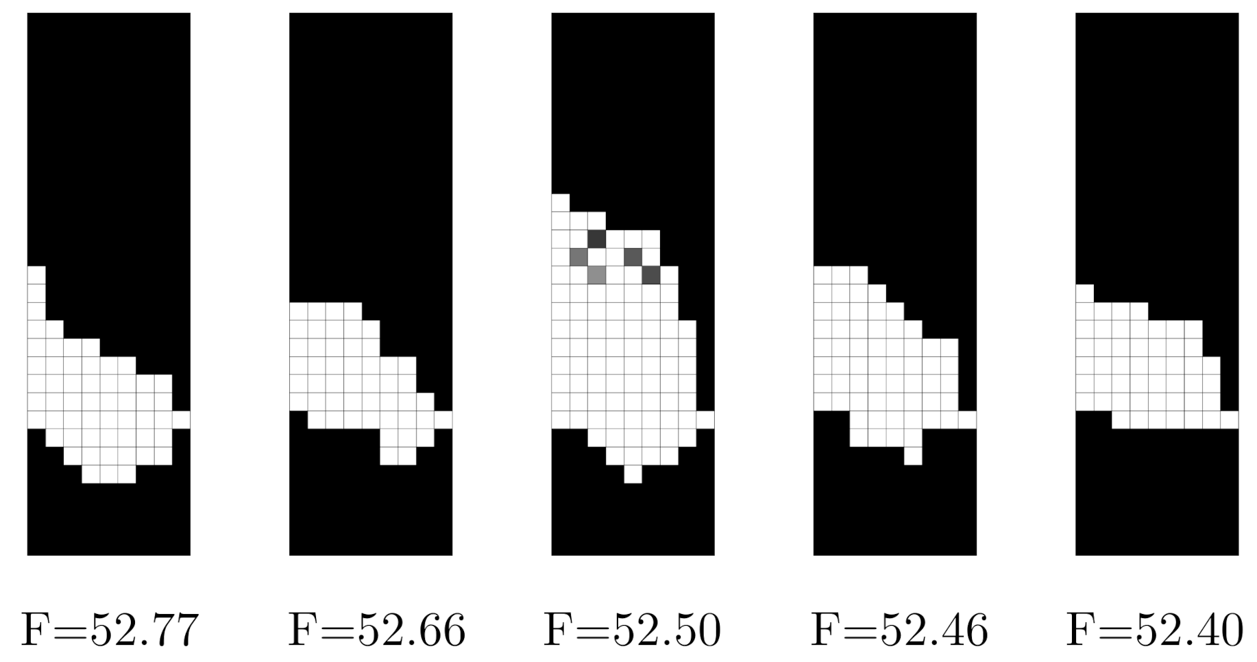
Figure 22 shows the topologies of the five best solutions obtained (the first two bars on the right of the histogram on the left of Figure 21) with the corresponding values of the force.

On the one hand, Figure 21 and Figure 22 highlight the multimodality of the problem, since there were various solutions for different initial points. The choice of the initial point highly impacted the final solution; nevertheless, all the solutions had force values that were higher than the initial electromagnet shown in Figure 19.

On the other hand, some solutions presented an intermediate material and a checkerboard pattern, as shown for the middle topology of Figure 22 and the integrity violation histogram of Figure 21; these problems require special treatment. In the literature, many filters were introduced to cope with these numerical instabilities [32,33,34]. The usage of these filters was not considered for these solutions, since the best one was satisfactory.

The cost of the optimization was estimated by the number of evaluations of the finite element code and the adjoint variable code, which were the most time consuming since the overhead introduced by the algorithm was negligible. The number of evaluations performed for the 31 optimization was 8504, which corresponds to around 275 evaluations for each optimization.

It is worth noting that the problem was solved using GA while considering the variables as integers; the solution obtained had a force value equal to 52.73 N/m and the number of evaluations 15,489.

Multi-Material Problem

As for the multi-material, to solve the optimization problem, we used a multistart SQP assisted by the adjoint variable method and GA.

The results of the multi-start SQP are shown in Figure 23 and Figure 24. The same observations were present as the previous problems except for the high number of cells that were in the intermediate material, as seen on the right; almost all the solutions had between 500 and 700 cells that had an intermediate material. Hence, all the solutions were not satisfactory, and new methodologies need to be considered.

As for GA, the algorithm was not able to converge even after more than 500,000 evaluations, and the returned value of the objective function was 0.01 N/m. The cause of this failure can be related to many aspects, such as the variables that were considered as binary or the large number of variables (6300) or the equality constraint in the problem. In the authors’ opinion, the most probable cause is the last one, since GA adopts a penalty constraint handling method, which is not well suited for equality constraints.

A simple filter was applied to the solutions obtained by SQP. It is somewhat similar to the rounding for unconstrained problems. Indeed, we formulated an integer linear problem from the initial problems. As the constraints were already linear, no special treatment was needed; however, for the objective function, we considered the solution of the optimization using SQP denoted $p_{ij}^{*}$, and we looked for the closest solution p that satisfied the constraints. Mathematically, the integer linear optimization problem is formulated as follows:

$$\begin{array}{c}\hfill \underset{\mathbf{p}}{\min }\sum _{j=1}^3\sum _{i=1}^{2100}(1-2p_{ji}^{*})p_{ji}\\ \hfill \mathrm{s}.\mathrm{t}.\sum _{i=1}^{2100}{p}_{1i}\le 1197\\ \hfill \sum _{i=1}^{2100}{p}_{2i}\le 210\\ \hfill \sum _{i=1}^{2100}{p}_{2i}=\sum _{i=1}^{2100}{p}_{3i}\\ \hfill p_{1i}+p_{2i}+p_{3i}\le 1,i=1,\dots ,2100\\ \hfill p_{1i},p_{2i},p_{3i}\in \{0,1\},i=1,\dots ,2100.\end{array}$$

(69)

Solving this problem did not require any expensive evaluation of the FEA. It generally converged only after one iteration using intlinprog (Mathworks Optimization Toolbox).

The solutions are shown in Figure 25. As can be seen on the right histogram, no solution violated the integrity constraints, while the values of the forces were almost the same as for Figure 23.

In Figure 26, we show the same topologies from Figure 24 after filtering.

5.4.4. Discussion

Multi-material optimization improved the design by a 39% increase in force compared to the original design and only 23% for the mono-material optimized device. Hence, multi-material device offered more gains for the optimization with many more degrees of freedom.

As for the algorithms’ comparison, although both topologies were different for the mono-material problem, they resulted in almost the same value of the force F. However, GA needed more evaluations. For the multi-material device, SQP with the filter outperformed GA thanks to the gradient computed using the adjoint variable method and the constraint handling technique used in SQP. On the other hand, GA performed poorly because of the additional constraints, essentially the one that imposed current conservation.

The multi-material optimized device was more prone to have intermediate materials than mono-material when no filter was considered. Therefore, further analysis needs to be conducted in this direction to exploit different filters mostly used in structural mechanics and adapt them to electromagnetic simulation.

6. Summary and Future Work

This paper presented a general verified adjoint variable method and how it can be applied to electromagnetic modeling. The formulation is valid for linear and nonlinear problems and can be extended to transient analysis with ease.

We developed an efficient way to compute the derivatives of the shape sensitivities, which are vital for the computation of the gradient. Sometimes, the finite-difference could be used with a mesh morphing strategy for computing the gradient. However, it can have an inhibitory effect since the mesh displacement is not always straightforward and can lead to a non-conforming mesh. The adjoint variable method was compared to the finite-difference to validate and highlight its precision and computational time effectiveness. Moreover, additional testing was performed in the context of optimization; the method showed its superiority compared to conventional approaches.

However, the gradient calculation with respect to geometrical variables using the adjoint variable method relied mainly on shape sensitivities. The geometric parameterization of shape variables is still one of the shortcomings of the method. We presented an approach based on the parametric equation of the geometric shapes; however, for very complex shapes, this can be very cumbersome. Some researchers use dedicated tools that couple the CAD software with the optimizer [35,36], such as The Computational Analysis PRogramming Interface (CAPRI) [37]. CAPRI serves the purpose of providing custom communications from a computational software suite to the preferred CAD system. This formalism allows the designer access to the CAD system’s geometry definitions and functionalities, providing the ability to query the CAD system whenever needed. Using this tool will enable us to automatically compute the shape sensitivities related to variables from the CAD software.

As regards the perspective of this work, we aim at applying this to the optimization of an electrical machine that has more geometric details than the test cases. Then, we have to add more realistic constraints on the geometry and the performances.