A Neural Controller for Induction Motors: Fractional-Order Stability Analysis and Online Learning Algorithm

Abstract

In this study, an intelligent control scheme is developed for induction motors (IMs). The dynamics of IMs are unknown and are perturbed by the variation of rotor resistance and load changes. The control system has two stages. In the identification stage, the group method of data-handling (GMDH) neural network (NN) was designed for online modeling of the IM. In the control stage, the GMDH-NN was applied to compensate for the impacts of disturbances and uncertainties. The stability is shown by the Lyapunov approach. Simulations demonstrated the good accuracy of the suggested new control approach under disturbances and unknown dynamics.

1. Introduction

The use of IMs has been a routine practice in industrial applications.The main reason is their simplicity, acceptable efficiency, good reliability, and low cost [1]. Various techniques have been developed to control the IMs in the past few decades. One of the important controllers is the field-oriented approach [2,3]. The other basic controller that is frequently applied for IMs is the PI controller [4]. The model predictive control technique was studied in [5], to investigate the performance of IMs at high and low speed. The other simple technique that is used for IMs is the vector control approach [6]. These methods are not robust under external disturbances and IM uncertainties and also depend on the mathematical dynamics.

To tackle the uncertainties in the dynamics of IMs, the sliding-mode controller (SMC) has been suggested in most studies [7]. The SMC is simple and robust. However, the switching term leads to the chattering phenomena in the control signal. In [8], the robust vector control method was designed for induction motors. In [9], the control method based on the high-order SMC was suggested. In order to resolve the chattering issue, a boundary layer scheme was developed in [10]. The vector control of the IM by the sliding mode method was studied in [11]. The nonsingular terminal SMC by means of a mathematical model of the IM and the principles of field orientation control was studied in [12]. To enhance the robustness, a disturbance rejection method on the basis of $H_{\infty }$ criteria was studied in [13,14]. In [15], an adaptive controller was formulated for the speed control of an IM, and its accuracy was studied in using the feedback linearization technique.

In most IM control schemes, it is presumed that the mathematical information of the IM is known, and only the impact of the parametric uncertainties is investigated. To cope with the perturbations of IMs, some NN-based controllers have been presented [16,17]. For example, in [18], the neural-network (NN)-based control method was applied to an IM where the parameters of the NN were trained by the Levenberg–Marquardt algorithm such that the accuracy of the vector method was increased. In [19], the speed controller was constructed by a TSK-based fuzzy system. In [20], based on fuzzy systems (FSs), a state feedback linearization technique was developed. An FS-based speed controller was designed in [21], in which the suitable rules were extracted by NNs and a backpropagation algorithm. In [22], an FS-based speed control scheme was constructed on the basis of the backtracking search method. A controller based on the fuzzy SMC was presented in [23], in which a fuzzy NN was suggested for the estimation of the nonlinearities. In [24], the speed control of an IM was investigated with respect to a particle swarm optimization algorithm. The fuzzy indirect control of an IM was studied in [25].

When standardized form regressions reached a dead end due to the complexity of the computations and the problem of linear dependence, in 1996, Ivakhnenko introduced a technique for constructing a highly simple polynomial called the GMDH algorithm or data organization method. This method is ideal for complex systems with an uncertain structure. Ivakhnenko’s algorithm is an exploratory method that extracts knowledge from the nature of the data and, as in regression analysis, is not based on a fixed theoretical foundation. A major problem in modeling complex systems in which the behavioral process and data structure are unclear is the issue of bias about the model structure. The main idea of the GMDH algorithm is to design a complex optimal model that only designs the model based on data and information and does not have any theoretical background on how the data work. This is done only on the basis of discovering a relationship between the input and output data of the system. Therefore, the GMDH algorithm builds a self-regulating model that has the ability to solve problems such as modeling, prediction, diagnosis, and control problems [26].

GMDH-NNs have been widely used in various applications. For example, in [27], a new voltage regulation system was designed, and a GMDH-NN was used for the estimation of the dynamics of the converters. In [28], a landslide mapping technique was presented by the use of GMDH-NNs, and it was shown that the GMDH-NNs resulted in better accuracy than the conventional approaches. In [29], a GMDH-NN was used to forecast the penetration rate in tunnel-boring machines, and by comparison with various regression methods, the capability of the GMDH-NN was studied. In [30], GMDH-NNs were used in a modeling problem, and their accuracy was examined with respect to other NNs. Furthermore, GMDH-NNs have been used in estimation problems such as the estimation of the wear rate of diamond wire [31], the capacity approximation of ferrocement members [32], blood pressure estimation [33], flood flow estimation [34], and the estimation of the compressibility of natural gas [35], among many others. In the most of the above applications, GMDH-NNs were used in an off-line optimization scheme, and the online control applications of GMDH-NNs have been seldom studied. In this study, some online learning rules are presented for GMDH-NNs in an online control application.

In the past few decades, fractional-order controllers have attracted increasing attention. It has been revealed that the fractional-order controllers result in a good performance in contrast to the integer-order ones [36]. However, the fractional-order controllers for IMs have rarely been studied. For instance, in [37], an observer was constructed using the integral SMC for the IMs. The fractional SMC was also investigated in [38]. The fractional-order PI control method was investigated in [39], and its efficiency was analyzed with respect to the traditional PI controller. In [40], it was practically proven that the fractional-order PID gives better accuracy with respect to the integer-order one. In [41], the rotor skin effect was modeled by fractional-order calculus. In [42], the application of IMs in robotic systems was investigated, and a fractional controller tuned by the particle swarm optimization method was proposed. In [43], the performance of the fractional- and integer-order proportional/integral controllers was compared by applying them to an IM. In [44], the fractional sliding mode strategy was studied for IMs, and its effectiveness was shown by a practical implementation. A fractional PI control system was designed in [45] for IMs on the basis of the Pareto-based optimization algorithm. The vibration of IMs with fractional PID control systems was studied in [46]. The robust neural-based control of IMs was investigated in [47].

The main contributions of the designed controller are as follows:

• A new fractional-order intelligent control approach is introduced using the proposed GMDH-NN;
• The IM dynamics are unknown and are disturbed by different faults, such as the variation of the unknown load torque and uncertain rotor resistance;
• The closed-loop stability was investigated, and a compensator was constructed to eradicate the impacts of IM perturbations;
• Adaptive learning rules are presented for GMDH-NNs.

2. Problem Formulation

2.1. System Dynamics

The IM dynamics are [48]:

$$\left\{\begin{array}{c}\frac{d\omega }{dt}=\mu {\varphi }_r{i}_{sq}-\frac{n_p{T}_r}{J}\hfill \\ \frac{d{\varphi }_r}{dt}=-\frac{1}{{\tau }_r}{\varphi }_r+\frac{M_{sr}}{{\tau }_r}{i}_{sq}\hfill \\ \frac{d{i}_{sd}}{dt}=\frac{\beta }{{\tau }_r}{\varphi }_{rd}+\beta \omega {\varphi }_{rq}-\frac{1}{{\tau }_1}{i}_{sd}+{\omega }_s{i}_{sd}\hfill \\ \frac{d{i}_{sq}}{dt}=\frac{\beta }{{\tau }_r}{\varphi }_{rq}-\beta \omega {\varphi }_{rd}-\frac{1}{{\tau }_1}{i}_{sq}-{\omega }_s{i}_{sd}+\frac{1}{L_1}{V}_{sq}\hfill \end{array}\right.$$

(1)

where ${\varphi }_r$ represents the rotor flux, (${\varphi }_{rd}$/${\varphi }_{rq}$) is the rotor flux, ($i_{rq}$/$i_{sq}$) is the stator current, and $V_{sq}$ indicates the stator voltage. ${\omega }_s$/$\omega$ denotes the angular frequency/rotor speed. $T_r$ shows is load torque. Other parameters are as follows:

$$\begin{array}{c}{\tau }_r=\frac{L_r}{R_r};L_1=L_s-\frac{{M_{sr}}^2}{L_r};R_1=R_s+R_r{\left(\frac{M_{sr}}{L_r}\right)}^2;\hfill \\ \beta =\frac{M_{sr}}{L_r{L}_1};\mu ={n^2}_p\left(\frac{M_{sr}}{J{L}_r}\right);{\tau }_1=\frac{L_1}{R_1}\hfill \end{array}$$

(2)

where J denotes the moment of inertia, $M_{sr}$ shows the mutual inductance, $n_p$ indicates the quantity of pole pairs, and $(R_s,R_r)/(L_s,L_r)$ are the resistances/inductances.

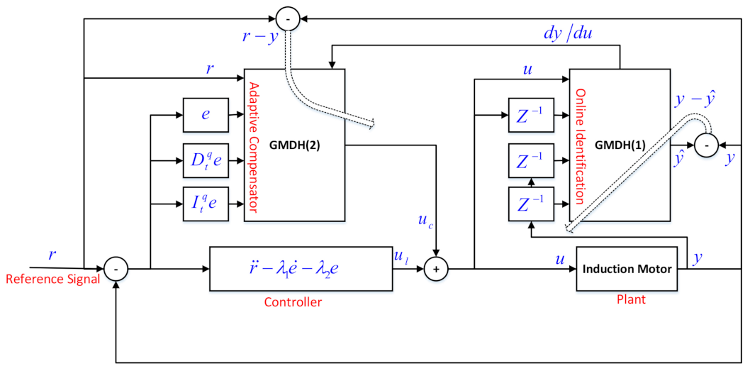
2.2. A General View of the Proposed Controller

The problem was to design a speed controller for IMs. The dynamics of IMs are considered completely uncertain. GMDH-NNs were used to estimate the dynamics of IMs, and based on the estimated model, a new fractional-order controller was designed. From (1), we can write:

$$\begin{array}{c}{\dot{x}}_1=f_1(\underset{\overline{}}{x})\hfill \\ {\dot{x}}_2=f_2(\underset{\overline{}}{x})\hfill \\ {\dot{x}}_3=f_3(\underset{\overline{}}{x})\hfill \\ {\dot{x}}_4=f_4(\underset{\overline{}}{x})+\frac{1}{L_1}u\hfill \end{array}$$

(3)

where,

$$\begin{array}{c}{f}_1(\underset{\overline{}}{x})=\mu {\varphi }_r{i}_{sq}-\frac{n_p{T}_r}{J},\hfill \\ f_2(\underset{\overline{}}{x})=-\frac{1}{{\tau }_r}{\varphi }_r+\frac{M_{sr}}{{\tau }_r}{i}_{sd}\hfill \\ f_3(\underset{\overline{}}{x})=\frac{\beta }{{\tau }_r}{\varphi }_r-\frac{1}{{\tau }_1}{i}_{sd}+{\omega }_s{i}_{sq},\hfill \\ f_4(\underset{\overline{}}{x})=-\beta \omega {\varphi }_r-\frac{1}{{\tau }_1}{i}_{sq}-{\omega }_s{i}_{sd}\hfill \\ u=V_{sq},x_1=\omega ,x_2={\varphi }_r,x_3=i_{sd},\hfill \\ x_4=i_{sq},\underset{\overline{}}{x}={\left[x_1,...,x_4\right]}^T\hfill \end{array}$$

(4)

The control aim was to plan a signal u in such a way that the output $y=x_1$ tracks the reference signal r. The suggested diagram is given in Figure 1. The term $D_t^{q}e$/$I_t^{q}e$ denotes the fractional-order derivative/integral based on the Caputo approach [49]:

$$D_t^{q}e\left(t\right)=\frac{1}{\Gamma (m-q)}{\int }_0^t{(t-\tau )}^{m-q-1}\frac{d^m}{d{\tau }^m}e\left(\tau \right)d\tau$$

(5)

$$I_t^q\Delta e\left(t\right)=\frac{1}{\Gamma \left(q\right)}{\int }_0^t{(t-\tau )}^{q-1}e\left(\tau \right)d\tau$$

(6)

where $m=1$ and $0<q<1$.

The time derivative of $\dot{w}$ in (1) yields:

$$\ddot{y}=\mu x_4{f}_2\left(\underline{x}\right)+\mu x_2{f}_4\left(\underline{x}\right)+\frac{\mu x_2}{L_1}u$$

(7)

where y denotes the output (see $\omega$ in (1)) and the other parameters are defined in (2) and (4). By considering (7), the control signal u based on the feedback linearization method can be designed as follows:

$$u=\frac{L_1}{\mu x_2}\left(-\mu x_4{f}_2\left(\underline{x}\right)-\mu x_2{f}_4\left(\underline{x}\right)+\ddot{r}-{\lambda }_1\dot{e}-{\lambda }_{2}e\right)$$

(8)

where ${\lambda }_i,i=1,2$ are constants and $e=r-y$. Considering Equation (8) and by the use of a learnable GMDH-NN, to achieve a stable controller, the control signal is suggested as follows:

$$u=\ddot{r}-{\lambda }_1\dot{e}-{\lambda }_{2}e-u_c$$

(9)

where $u_c$ is the output of the GMDH(2). The parameters of the compensator GMDH(2) were tuned in such a way that $e=r-y$ was minimized. To tune the parameters of the GMDH(2) based on the error e, the output derivative regarding the control signal is required ($dy/\phantom{dydu}du$). The term $dy/\phantom{dydu}du$ is obtained from online modeling of the system by the GMDH(1).

3. Proposed GMDH Neural Network

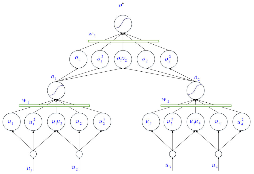
3.1. Structure

In this section, the proposed neural networks structure is illustrated. It has been shown that GMDH-NNs result in better accuracy in contrast to other conventional NNs such as multi-layer perceptrons [50]. GMDH neural networks have a better nonlinear nature and are more proper for the estimation of the complicated nonlinear functions. The structure of the proposed GMDH neural network with four inputs is shown in Figure 2. The vector of the parameters in the GMDH(1) and GMDH(2) are denoted by $w{1}_j$ and $w{2}_j$, $j=1,2,3$, respectively. The outputs of the GMDH(1) and GMDH(2) are obtained as follows:

Step 1:

The vectors of the inputs for the GMDH(1) and GMDH(2) are $[u\left(t\right),u\left(t-1\right),y\left(t\right),$$y\left(t-1\right){]}^T$ and $[r\left(t\right),e\left(t\right),D_t^{q}e\left(t\right),I_t^{q}e\left(t\right){]}^T$, respectively. One of the characteristics of the suggested controller is that it uses the minimum information of the system. To identify the dynamics of the IM, only the input–output datasets are used. It should be noted that by the use of the GMDH(1), we wanted to obtain the control direction;

Step 2:

Compute the outputs of the hidden layers for the GMDH(1) and GMDH(2) as follows:

$$\begin{array}{c}o{1}_1=f{1}_1\left(h{1}_1\right),o{1}_2=f{1}_1\left(h{1}_2\right)\hfill \\ o{2}_1=f{2}_1\left(h{2}_1\right),o{2}_2=f{2}_1\left(h{2}_2\right)\hfill \end{array}$$

(10)

where $f{1}_1$/$f{2}_1$ denotes the activation function in the first layer for the GMDH(1)/GMDH(2), which is defined as follows:

$$f{1}_1\left(h\right)=f{2}_1\left(h\right)=\frac{1-exp\left(-h\right)}{1+exp\left(-h\right)}$$

(11)

The other parameters $h{1}_1$, $h{1}_2$, $h{2}_1$, and $h{2}_2$ are computed as follows:

$$\begin{array}{c}h{1}_1=w{1}_1^T\zeta 1_1,h{1}_1=w{1}_2^T\zeta 1_2\hfill \\ h{2}_1=w{2}_1^T\zeta 2_1,h{2}_1=w{2}_2^T\zeta 2_2\hfill \end{array}$$

(12)

where,

$$\begin{array}{c}\zeta 1_1=\hfill \\ {\left[u\left(t\right),u^2\left(t\right),u\left(t\right)u\left(t-1\right),u\left(t-1\right),u^2\left(t-1\right)\right]}^T,\hfill \\ \zeta 1_2=\hfill \\ {\left[y\left(t-1\right),y^2\left(t-1\right),y\left(t-1\right)y\left(t-2\right),y\left(t-2\right),y^2\left(t-2\right)\right]}^T\hfill \end{array}$$

(13)

$$\begin{array}{c}\zeta 2_1=\hfill \\ {\left[r\left(t\right),r^2\left(t\right),r\left(t\right)e\left(t\right),e\left(t\right),e^2\left(t\right)\right]}^T,\hfill \\ \zeta 2_2=\hfill \\ {\left[D_t^{q}e\left(t\right),{\left(D_t^{q}e\left(t\right)\right)}^2,D_t^{q}e\left(t\right)I_t^{q}e\left(t\right),I_t^{q}e\left(t\right),{\left(I_t^{q}e\left(t\right)\right)}^2\right]}^T;\hfill \end{array}$$

(14)

Step 3:

Compute the outputs of the GMDH(1) and GMDH(2) as follows:

$$\begin{array}{c}{Y}_1=f{1}_2\left(h{1}_3\right),\hfill \\ Y_2=f{2}_2\left(h{2}_3\right)\hfill \end{array}$$

(15)

where $Y_1$ and $Y_2$ are the output of the GMDH(1) and GMDH(2), respectively, and:

$$\begin{array}{c}f{1}_2\left(h{1}_3\right)=h{1}_3\hfill \\ f{2}_2\left(h{2}_3\right)=\overline{E}\mathrm{sign}\left({\underline{e}}^{T}Pb\right)\left[1+exp\left(h{2}_3\right)\right]\hfill \end{array}$$

(16)

$$h{1}_3=w{1}_3^T\zeta 1_3,h{2}_3=w{2}_3^T\zeta 2_3$$

(17)

$$\begin{array}{c}\zeta 1_3={\left[o{1}_1,o{1}_1^2,o{1}_{1}o{1}_2,o{1}_2,o{1}_2^2\right]}^T\hfill \\ \zeta 2_3={\left[o{2}_1,o{2}_1^2,o{2}_{1}o{2}_2,o{2}_2,o{2}_2^2\right]}^T\hfill \end{array}$$

(18)

where $\overline{E}$ is the designable constant parameter. The value of $\overline{E}$ is determined considering the above bound of the uncertainties. ${\underline{e}}^{T}Pb$ is defined in (44)–(46).

3.2. Learning of the GMDH(1)

The parameters of the GMDH(1) are updated such that (19) is minimized:

$${\displaystyle J_1=\frac{1}{2}{\left(y-Y_1\right)}^2}$$

(19)

where y is the system output and $Y_1$ represents the output of the GMDH(1). The adaptation laws are as follows:

$$\begin{array}{c}{\displaystyle w{1}_1\left(t+1\right)=w{1}_1\left(t\right)-\eta \frac{\partial J_1}{\partial w{1}_1}}\hfill \\ {\displaystyle w{1}_2\left(t+1\right)=w{1}_2\left(t\right)-\eta \frac{\partial J_1}{\partial w{1}_2}}\hfill \\ {\displaystyle w{1}_3\left(t+1\right)=w{1}_3\left(t\right)-\eta \frac{\partial J_1}{\partial w{1}_3}}\hfill \end{array}$$

(20)

where $\eta$ is the adaptation rate. $\frac{\partial J_1}{\partial w{1}_i},i=1,2,3$ is computed as follows:

$$\begin{array}{c}{\displaystyle \frac{\partial J_1}{\partial w{1}_3}=\frac{\partial J_1}{\partial Y_1}\frac{\partial Y_1}{\partial h{1}_3}\frac{\partial h{1}_3}{\partial w{1}_3}}\hfill \\ =-\left(y-Y_1\right)\zeta 1_3\hfill \end{array}$$

(21)

$$\begin{array}{c}\frac{\partial J_1}{\partial w{1}_2}=\frac{\partial J_1}{\partial Y_1}\frac{\partial Y_1}{\partial o{1}_2}\frac{\partial o{1}_2}{\partial h{1}_2}\frac{\partial h{1}_2}{\partial w{1}_2}\hfill \\ \begin{array}{c}=-\left(y-Y_1\right)\times \hfill \\ \left(w{1}_{33}o{1}_1+w{1}_{34}+2w{1}_{35}o{1}_2\right)\frac{\partial f{1}_1}{\partial h{1}_2}\zeta 1_2\hfill \end{array}\hfill \end{array}$$

(22)

$$\begin{array}{c}\frac{\partial J_1}{\partial w{1}_1}=\frac{\partial J_1}{\partial Y_1}\frac{\partial Y_1}{\partial o{1}_1}\frac{\partial o{1}_1}{\partial h{1}_1}\frac{\partial h{1}_1}{\partial w{1}_1}\hfill \\ \begin{array}{c}=-\left(y-Y_1\right)\times \hfill \\ \left(w{1}_{31}+2w{1}_{32}o{1}_1+w{1}_{33}o{1}_2\right)\frac{\partial f{1}_1}{\partial h{1}_1}\zeta 1_1\hfill \end{array}\hfill \end{array}$$

(23)

where $w{1}_{3j},j=1,\dots ,5$ denotes the $j-th$ element of the vector $w{1}_3$ and $\frac{\partial f{1}_1}{\partial h{1}_i},i=1,2$ is:

$${\displaystyle \frac{\partial f{1}_1}{\partial h{1}_i}=\frac{2exp\left(-h{1}_i\right)}{1+exp\left(-h{1}_i\right)},i=1,2}$$

(24)

To show the fact that the tuning rules (20) minimize the cost function (19), it is proven that the difference of (19) is negative. Then,

$$\Delta J_1\left(t\right)=J_1\left(t+1\right)-J_1\left(t\right)$$

(25)

Consider the following definition:

$$\begin{array}{c}e\left(t+1\right)=e\left(t\right)+\Delta e\left(t\right)\cong e\left(t\right)\hfill \\ +{\left[\frac{\partial e}{\partial w{1}_1}\right]}^T\Delta w{1}_1+{\left[\frac{\partial e}{\partial w{1}_2}\right]}^T\Delta w{1}_2+{\left[\frac{\partial e}{\partial w{1}_3}\right]}^T\Delta w{1}_3\hfill \end{array}$$

(26)

where,

$$e=y-Y_1$$

(27)

From (20), it can be concluded that:

$$\Delta w{1}_i\left(t\right)=-\eta \frac{\partial e}{\partial w{1}_i}e\left(t\right),i=1,2,3$$

(28)

$\Delta J_1\left(t\right)$ in (25) can be rewritten as:

$$\begin{array}{c}\Delta J_1\left(t\right)=\frac{1}{2}\left(e\left(t+1\right)-e\left(t\right)\right)\left(e\left(t+1\right)+e\left(t\right)\right)\hfill \\ =\frac{1}{2}\Delta e\left(t\right)\left(2e\left(t\right)+\Delta e\left(t\right)\right)\hfill \end{array}$$

(29)

By substituting $\Delta e\left(t\right)$ from (26), we have:

$$\begin{array}{c}\Delta J_1\left(t\right)=\frac{1}{2}\left({\left[\frac{\partial e}{\partial w{1}_1}\right]}^T\Delta w{1}_1+{\left[\frac{\partial e}{\partial w{1}_2}\right]}^T\Delta w{1}_2+{\left[\frac{\partial e}{\partial w{1}_3}\right]}^T\Delta w{1}_3\right)·\hfill \\ \left(2e\left(t\right)+{\left[\frac{\partial e}{\partial w{1}_1}\right]}^T\Delta w{1}_1+{\left[\frac{\partial e}{\partial w{1}_2}\right]}^T\Delta w{1}_2+{\left[\frac{\partial e}{\partial w{1}_3}\right]}^T\Delta w{1}_3\right)\hfill \end{array}$$

(30)

Equation (30) is rewritten as:

$$\Delta J_1\left(t\right)=-\frac{1}{2}{e}^2\left(t\right)\left(\eta \sum _{i=1}^3{\left[\frac{\partial e}{\partial w{1}_i}\right]}^T\frac{\partial e}{\partial w{1}_i}\right)·\left(-2+\eta \sum _{i=1}^3{\left[\frac{\partial e}{\partial w{1}_i}\right]}^T\frac{\partial e}{\partial w{1}_i}\right)$$

(31)

Then, $\Delta J_1\left(t\right)<0$, if:

$$\eta <\frac{2}{{\displaystyle \sum _{i=1}^3}{\left[\frac{\partial e}{\partial w{1}_i}\right]}^T\frac{\partial e}{\partial w{1}_i}}$$

(32)

3.3. Learning of the GMDH(2)

The parameters of the GMDH(2) are adjusted such that (33) is minimized.

$$J_2=\frac{1}{2}{\left(r-y\right)}^2$$

(33)

where r indicates the reference and y shows the output. The adaptation laws for the parameters $w{2}_1$, $w{2}_2$, and $w{2}_3$ are obtained as follows:

$$\begin{array}{c}{\displaystyle w{2}_1\left(t+1\right)=w{2}_1\left(t\right)-\eta \frac{\partial J_2}{\partial w{2}_1}}\hfill \\ {\displaystyle w{2}_2\left(t+1\right)=w{2}_2\left(t\right)-\eta \frac{\partial J_2}{\partial w{2}_2}}\hfill \\ {\displaystyle w{2}_3\left(t+1\right)=w{2}_3\left(t\right)-\eta \frac{\partial J_2}{\partial w{2}_3}}\hfill \end{array}$$

(34)

where $\eta$ is the adaptation rate. The term $\frac{\partial J_2}{\partial w{2}_3}$ is determined as follows:

$$\begin{array}{c}\frac{\partial J_2}{\partial w{2}_3}=\frac{\partial J_2}{\partial y}\frac{\partial y}{\partial u}\frac{\partial u}{\partial Y_2}\frac{\partial Y_2}{\partial h{2}_3}\frac{\partial h{2}_3}{\partial w{2}_3}\hfill \\ =-\left(r-y\right)\frac{\partial y}{\partial u}\frac{\partial f{2}_3}{\partial h{2}_3}\zeta 2_3\hfill \end{array}$$

(35)

where,

$$\frac{\partial f{2}_3}{\partial h{2}_3}=\overline{E}\mathrm{sign}\left({\underline{e}}^{T}Pb\right)exp\left(h{2}_3\right)$$

(36)

The term $\frac{\partial y}{\partial u}$ in (35) is estimated by $\frac{\partial Y_1}{\partial u}$, where:

$$\begin{array}{c}\frac{\partial Y_1}{\partial u}=\frac{\partial Y_1}{\partial h{1}_3}\frac{\partial h{1}_3}{\partial o_1}\frac{\partial o_1}{\partial h{1}_1}\frac{\partial h{1}_1}{\partial u}\hfill \\ \begin{array}{c}=\left(w{1}_{31}+2w{1}_{32}o{1}_1+w{1}_{33}o{1}_2\right)\times \hfill \\ \frac{\partial f{1}_1}{\partial h{1}_1}\left(w{1}_{11}+2w{1}_{12}u\left(t\right)+w{1}_{13}o{1}_{2}u\left(t-1\right)\right)\hfill \end{array}\hfill \end{array}$$

(37)

where $w{1}_{3j}$ and $w{1}_{1j},j=1,\dots ,5$, represent the $j-th$ element in the vectors $w{1}_3$ and $w{1}_1$, respectively. $w{1}_3$ and $w{1}_1$ in (37) are the parameters of the GMDH(1). Similar to (35), the terms $\frac{\partial J_2}{\partial w{2}_2}$ and $\frac{\partial J_2}{\partial w{2}_1}$ are determined as follows:

$$\begin{array}{c}\frac{\partial J_2}{\partial w{2}_2}=\frac{\partial J_2}{\partial y}\frac{\partial y}{\partial u}\frac{\partial u}{\partial Y_2}\frac{\partial Y_2}{\partial o{2}_2}\frac{\partial o{2}_2}{\partial w{2}_2}\hfill \\ \begin{array}{c}=-\left(r-y\right)\frac{\partial y}{\partial u}\frac{\partial f{2}_3}{\partial h{2}_3}\times \hfill \\ \left(w{2}_{33}o{2}_1+w{2}_{34}+2w{2}_{35}o{2}_2\right)\frac{\partial f{2}_1}{\partial h{2}_2}\zeta 2_2\hfill \end{array}\hfill \end{array}$$

(38)

$$\begin{array}{c}\frac{\partial J_2}{\partial w{2}_1}=\frac{\partial J_2}{\partial y}\frac{\partial y}{\partial u}\frac{\partial u}{\partial Y_2}\frac{\partial Y_2}{\partial o{2}_1}\frac{\partial o{2}_1}{\partial w{2}_1}\hfill \\ \begin{array}{c}=-\left(r-y\right)\frac{\partial y}{\partial u}\frac{\partial f{2}_3}{\partial h{2}_3}\times \hfill \\ \left(w{2}_{31}+2w{2}_{32}o{2}_1+w{2}_{33}o{2}_2\right)\frac{\partial f{2}_1}{\partial h{2}_1}\zeta 2_1\hfill \end{array}\hfill \end{array}$$

(39)

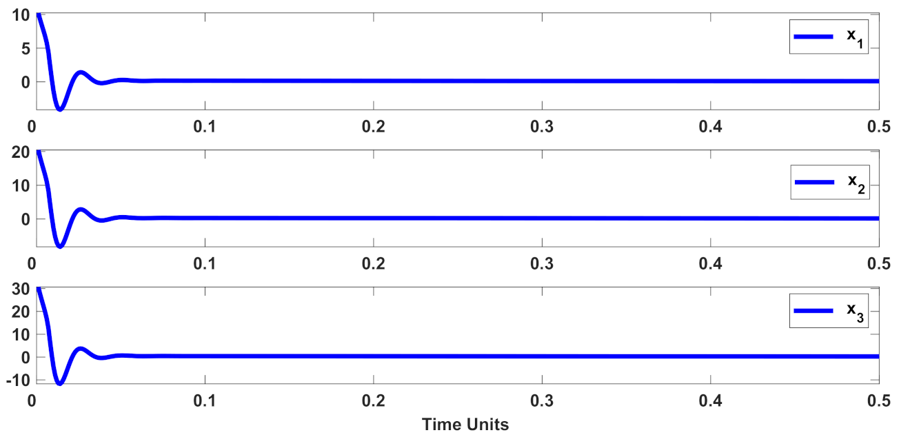
4. Stability Analysis

The dynamics in (7) is rewritten as:

$$\ddot{y}=F+Gu$$

(40)

where,

$$F=\mu x_4{f}_2\left(\underline{x}\right)+\mu x_2{f}_4\left(\underline{x}\right),G=\frac{\mu x_2}{L_1}$$

(41)

Then, by considering the proposed control signal, the error becomes:

$$\ddot{e}=F+\left(G-1\right)u-{\lambda }_1\dot{e}-{\lambda }_{2}e-Y_2$$

(42)

From (42), we have:

$$\underline{\dot{e}}=A\underline{e}+bE-b{Y}_2$$

(43)

where,

$$\begin{gathered} ={\left[\begin{array}{cc}\dot{e}& e\end{array}\right]}^T,A=\left[\begin{array}{cc}1& 0\\ -{\lambda }_1& -{\lambda }_2\end{array}\right] \\ b=\left[\begin{array}{c}0\\ 1\end{array}\right],E=F+\left(G-1\right)u \end{gathered}$$

(44)

For the stability investigation, the Lyapunov function (45) is considered:

$$V=\frac{1}{2}{\underline{e}}^{T}P\underline{e}$$

(45)

where P satisfies:

$$A^{T}P+PA=-Q$$

(46)

where Q is the arbitrary positive-definite function. The time derivative of V in (45) yields:

$$\dot{V}=-{\underline{e}}^{T}Q\underline{e}+{\underline{e}}^{T}PbE-{\underline{e}}^{T}Pb{Y}_2$$

(47)

From (47), we can write:

$$\dot{V}\le -{\underline{e}}^{T}Q\underline{e}+\left|{\underline{e}}^{T}Pb\right|\left|E\right|-\left|{\underline{e}}^{T}Pb\right|\mathrm{sign}\left({\underline{e}}^{T}Pb\right)Y_2$$

(48)

From (48), we have:

$$\dot{V}\le -{\underline{e}}^{T}Q\underline{e}+\left|{\underline{e}}^{T}Pb\right|\left(\left|E\right|-\mathrm{sign}\left({\underline{e}}^{T}Pb\right)Y_2\right)$$

(49)

From the fact that $Y_2=\overline{E}\mathrm{sign}\left({\underline{e}}^{T}Pb\right)\left[1+exp\left(h{2}_3\right)\right]>\left|E\right|$, $\dot{V}$ in (49) becomes:

$$\dot{V}\le -{\underline{e}}^{T}Q\underline{e}$$

(50)

Then, from (50), the closed-loop stability is proven.

Remark 1.

Although the upper bound of uncertainty can be conservatively considered big enough, by taking into account the characteristics of the controlled plant, the upper bound of uncertainty can be better specified. Furthermore, the upper bounds of the signals can be controlled by the use of saturation.

Remark 2.

In comparison with other conventional controllers such as PID [51], the SMC [52], and the model-based predictive controller [53], the suggested approach has a stability guarantee and robustness property against perturbations. It has an adaptive scheme, and it is also not dependent on the mathematical dynamics of IMs. It should be noted that, since the inputs of the GMDH(2) are the error, fractional derivative, and integral of the error, then it has also the property of conventional PIDs.

Remark 3.

The suggested controller is not dependent on the mathematical model of IMs. The required information is identified online (note that the GMDH(1) is used to extract the control direction). Furthermore, a compensator (GMDH(2)) is updated online to guarantee stability and robustness.

5. Simulation

To verify the efficiency, an IM was considered as 1.5 kW with a power supply of (380–220 V) for the cage rotor. Other mechanical constraints and conditions are described in

Table 1. The simulation parameters.

Parameter	Value	Units
$R_s$	1.20	$\Omega$
$L_r$	0.1569	H
$T_{rN}$	5	${\mathrm{N}}_{\mathrm{m}}$
-	1480	$\mathrm{r}\mathrm{p}\mathrm{m}$
$M_{sr}$	0.15	H
$L_s$	0.1555	H
$np$	2	-
J	0.013	$\mathrm{k}\mathrm{g}{\mathrm{m}}^2$
$R_r$	1.1	$\Omega$

and

Table 2. The control parameters.

${\mathit{\lambda }}_1$, ${\mathit{\lambda }}_2$	q	$\mathit{\eta }$	$\overline{\mathit{E}}$	$\underline{\mathit{E}}$
see (9)	see (Figure 1)	see (20) and (34)	see (16)	see (16)
50	0.9	0.1	100	−100

. The free parameters of GMDH-NNs were optimized online. The other parameters as mentioned in Table 2 were chosen based on the general information of the IM such as the upper/lower bounds of the uncertainties. The learning rate was selected small enough to have a smooth adaptation.

The tracking effectiveness and tracking error under the normal condition (unknown dynamics with nominal load torque (5 $N_m$) and normal rotor resistance) are displayed in Figure 3 and Figure 4. The quadrature and direct components of the stator current are shown in Figure 5 and Figure 6. Figure 7 gives the control signal. It is obvious that the presented control scenario gives the desired accuracy.

To examine the efficiency with respect to faulty conditions, the variation of the rotor resistance was considered as $R=R_N+R_N\left(-exp\left(-1.5t\right)+1\right)$, where $R_N$ indicates the nominal value of R. Furthermore, the load torque was also time variable, and it was changed at t = 20 s (see Figure 8). The rotor speed and tracking error are displayed in Figure 9 and Figure 10. Figure 11 and Figure 12 represent the stator currents. Figure 13 shows the control signal. The results showed that the designed control scenario had perfect accuracy under faulty conditions, as well as the dynamics’ perturbation. It is worth mentioning that, in addition to the aforementioned disturbances, the IM dynamics were presumed to be completely uncertain.

The tracking effectiveness of the suggested technique was analyzed with respect to other well-known techniques such as: the adaptive SMC (ASMC) [54], the fault-tolerant adaptive control (FTAC) approach [48], field-oriented control (FOC), as well as the adaptive type-2 fuzzy SMC (AST2FC) [55]. The output trajectories are shown in Figure 14.

Table 3. RMSE and ISE comparisons.

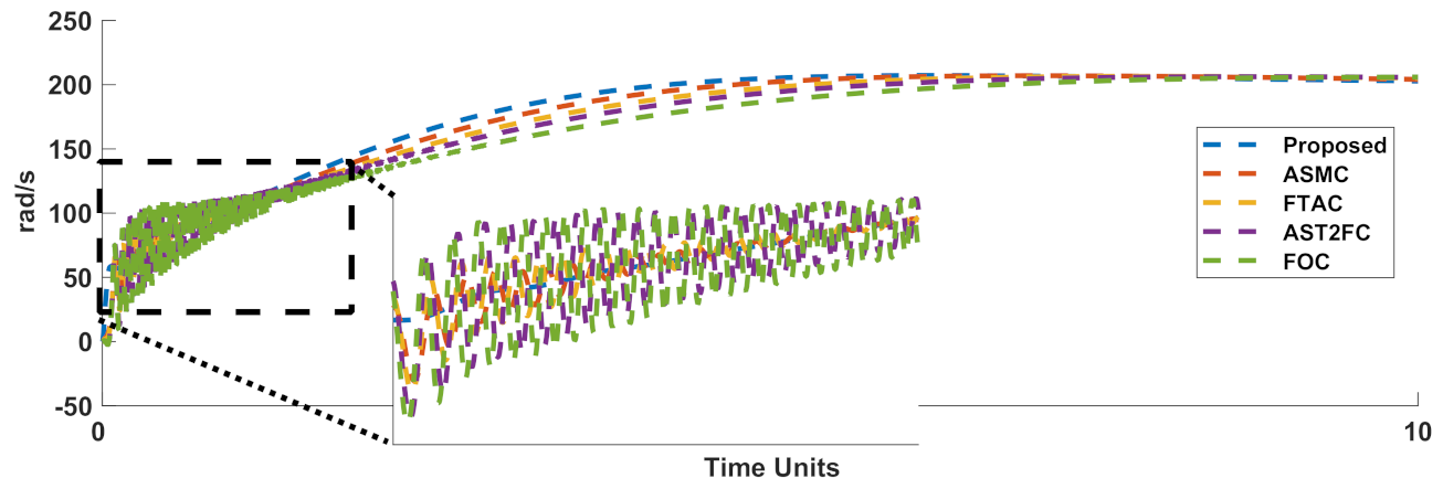
	FOC [48]	FTAC [48]	AST2FC [55]	ASMC [54]	Proposed Controller
RMSE	45.11	40.55	41.52	36.34	12.8085
ISE	4.5178 × 104	3.87124 × 104	3.78101 × 104	3.1427 × 104	1.1972 × 104

shows a comparison of the root-mean-squared errors (RMSEs) and the integral of the squared error (ISE). To compute the RMSE, the squares of the tracking error were saved, and at the end of the simulation, the root mean squareof the saved data was computed. The results indicated that the values of the RMSE and ISE for the suggested approach were meaningfully less than the other approaches. Furthermore, in

Table 4. Comparison of the RMSE for different values of the fractional orders.

q	0.5	0.7	0.8	0.9	0.95
RMSE	12.8284	12.8278	12.8217	12.8085	12.8203

, it is shown that the fractional-order controllerdid not strongly affect the accuracy. The results of Table 4, and the trajectories of the output regulation in Figure 3 and Figure 9 demonstrate the desired efficiency of the designed controller.

Furthermore, the effectiveness of the proposed compensator was examined in three cases. In Case 1, the compensator was eliminated. In Case 2, multi-layer perceptron (MLP) was used as the compensator. In Case 3, the proposed GMDH was employed as the compensator. In Case 4, the type-1 fuzzy system (T1FS) was used as the compensator.

Table 5. Comparison of the RMSE for different compensators.

	Without Compensator	MLP	T1FS	GMDH
w	696.8100	13.3709	13.10	12.8085

shows the values of the RMSE for different cases, which showed that the proposed compensator on the basis of the GMDH improved the tracking performance.

Remark 4.

The suggested control scenario was not dependent on the system’s mathematical information. Furthermore, the stability was ensured by the proposed compensator. Then, the designed controller could be used in many cases of nonlinear plants. To show this property, the designed control scheme was applied to nonlinear systems with the following unknown dynamics [56]:

$$\begin{array}{c}{D}^{\alpha }{x}_1=10\left(x_2-x_1\right)+u_1\hfill \\ D^{\alpha }{x}_2=40x_1-x_1{x}_3+u_2\hfill \\ D^{\alpha }{x}_3=-4x_1^2-2.5x_3+u_3\hfill \end{array}$$

(51)

where the initial states were $x_1\left(0\right)=11$, $x_2\left(0\right)=21$, and $x_3\left(0\right)=31$ and the control signals were considered as $u_i=\dot{r}-20e_i-u_{c_i}$, in which, $r=0$ and $e_i=x_i$. The performance is depicted in Figure 15. From Figure 15, we see that the suggested controller had the desired accuracy in spite of the unmown dynamics.

Remark 5.

The simulations were carried with MATLAB 2018a and an x64-based processor with CPU @2.60 GHz, RAM 8 GB Intel(R) Core(TM) i7-4720HQ. The fractional-order operator was simulated by the use of the Simulink block “nid”, presented by Duarter Valerio [57].

Remark 6.

The designed controller does not depend on the mathematical dynamics of the IM. However, an online scheme by the use of GMDH-NNs is suggested for modeling. Furthermore, the main perturbations in the practical application of IMs are supported by the designed compensator. The capability of the designed controller in a real environment was shown by various simulations, considering dynamic uncertainties and disturbances. The authors will implement the designed controller on a real IM in their future studies. The main drawbacks of the designed scheme are that the input delay and actuator faults are not considered. For future studies, the controller can be extended for other classes of nonlinear systems with more robustness against faults and disturbances.

6. Conclusions

In this study, an intelligent control method was introduced for the speed control of IMs. The IM dynamics were considered to be uncertain and also perturbed by changes in the rotor resistance and load torque. The stability was analyzed using the Lyapunov theorem. The designed controller was applied to an IM in both nominal and faulty scenarios. The simulation findings revealed that the suggested control scheme had perfect accuracy with respect to disturbances and perturbed dynamics. Furthermore, to examine the effectiveness in the other case of nonlinear systems, one more simulation was considered by controlling a chaotic system with unknown dynamics. The results demonstrated that the introduced approach had good accuracy in spite of its simplicity.

References

- Yin, H.; Yi, W.; Wu, J.; Wang, K.; Guan, J. Adaptive Fuzzy Neural Network PID Algorithm for BLDCM Speed Control System. Mathematics 2022, 10, 118. [Google Scholar] [CrossRef]
- Yin, H.; Yi, W.; Wang, K.; Guan, J.; Wu, J. Research on brushless DC motor control system based on fuzzy parameter adaptive PI algorithm. Aip Adv. 2020, 10, 105208. [Google Scholar] [CrossRef]
- Benbouhenni, H.; Bizon, N. Improved Rotor Flux and Torque Control Based on the Third-Order Sliding Mode Scheme Applied to the Asynchronous Generator for the Single-Rotor Wind Turbine. Mathematics 2021, 9, 2297. [Google Scholar] [CrossRef]
- Alvarez-Ramirez, J.; Fernandez, G.; Suarez, R. A PI controller configuration for robust control of a class of nonlinear systems. J. Frankl. Inst. 2002, 339, 29–41. [Google Scholar] [CrossRef]
- Sharma, D.; Nandanwar, V. Performance of induction motor at low and high speed using model predictive control method. Int. J. Res. Sci. Eng. 2016, 3, 779–785. [Google Scholar]
- Yu, X.; Dunnigan, M.W.; Williams, B.W. Comparative study of sliding mode speed and position control of a vector-controlled induction machine. Trans. Inst. Meas. Control 2001, 23, 83–101. [Google Scholar] [CrossRef]
- Benbouhenni, H.; Bizon, N. Third-Order Sliding Mode Applied to the Direct Field-Oriented Control of the Asynchronous Generator for Variable-Speed Contra-Rotating Wind Turbine Generation Systems. Energies 2021, 14, 5877. [Google Scholar] [CrossRef]
- Barambones, O.; Alkorta, P. A robust vector control for induction motor drives with an adaptive sliding-mode control law. J. Frankl. Inst. 2011, 348, 300–314. [Google Scholar] [CrossRef]
- Ammar, A.; Bourek, A.; Benakcha, A. Nonlinear SVM-DTC for induction motor drive using input–output feedback linearization and high order sliding mode control. ISA Trans. 2017, 67, 428–442. [Google Scholar] [CrossRef]
- Saghafinia, A.; Ping, H.W.; Uddin, M.N. Fuzzy sliding mode control based on boundary layer theory for chattering-free and robust induction motor drive. Int. J. Adv. Manuf. Technol. 2014, 71, 57–68. [Google Scholar] [CrossRef]
- Salih, Z.H.; Gaeid, K.S.; Saghafinia, A. Sliding Mode Control of Induction Motor with Vector Control in Field Weakening. Mod. Appl. Sci. 2015, 9, 276. [Google Scholar] [CrossRef] [Green Version]
- Feng, Y.; Zhou, M.; Zheng, X.; Han, F.; Yu, X. Terminal sliding-mode control of induction motor speed servo systems. In Proceedings of the 2016 14th International Workshop on Variable Structure Systems (VSS), Nanjing, China, 1–4 June 2016; pp. 351–355. [Google Scholar]
- Li, J.; Ren, H.P.; Zhong, Y.R. Robust speed control of induction motor drives using first-order auto-disturbance rejection controllers. IEEE Trans. Ind. Appl. 2015, 51, 712–720. [Google Scholar] [CrossRef]
- Pohl, L.; Vesely, I. Speed Control of Induction Motor Using H∞ Linear Parameter Varying Controller. IFAC-PapersOnLine 2016, 49, 74–79. [Google Scholar] [CrossRef]
- Talla, J.; Leu, V.Q.; Šmídl, V.; Peroutka, Z. Adaptive Speed Control of Induction Motor Drive With Inaccurate Model. IEEE Trans. Ind. Electron. 2018, 65. [Google Scholar] [CrossRef]
- Li, R.; Yang, L.; Chen, Y.; Lai, G. Adaptive Sliding Mode Control of Robot Manipulators with System Failures. Mathematics 2022, 10, 339. [Google Scholar] [CrossRef]
- Yang, L.; Lai, G.; Chen, Y.; Guo, Z. Online Control for Biped Robot with Incremental Learning Mechanism. Appl. Sci. 2021, 11, 8599. [Google Scholar] [CrossRef]
- Fu, X.; Li, S. A novel neural network vector control technique for induction motor drive. IEEE Trans. Energy Convers. 2015, 30, 1428–1437. [Google Scholar] [CrossRef]
- Wang, S.Y.; Tseng, C.L.; Chiu, C.J. Design of a novel adaptive TSK-fuzzy speed controller for use in direct torque control induction motor drives. Appl. Soft Comput. 2015, 31, 396–404. [Google Scholar] [CrossRef]
- Yousef, H.; Hamdy, M.; El-Madbouly, E.; Eteim, D. Adaptive fuzzy decentralized control for interconnected MIMO nonlinear subsystems. Automatica 2009, 45, 456–462. [Google Scholar] [CrossRef]
- Kusagur, A.; Fakirappa Kodad, S.; Ram, S. Modelling & Simulation of an ANFIS controller for an AC drive. World J. Model. Simul. 2012, 8, 36–49. [Google Scholar]
- Ali, J.A.; Hannan, M.; Mohamed, A.; Abdolrasol, M.G. Fuzzy logic speed controller optimization approach for induction motor drive using backtracking search algorithm. Measurement 2016, 78, 49–62. [Google Scholar] [CrossRef]
- Vahedi, M.; Hadad Zarif, M.; Akbarzadeh Kalat, A. Speed control of induction motors using neuro-fuzzy dynamic sliding mode control. J. Intell. Fuzzy Syst. 2015, 29, 365–376. [Google Scholar] [CrossRef]
- Mahapatra, S.; Daniel, R.; Dey, D.N.; Nayak, S.K. Induction motor control using PSO-ANFIS. Procedia Comput. Sci. 2015, 48, 753–768. [Google Scholar] [CrossRef] [Green Version]
- Uddin, M.N.; Radwan, T.S.; Rahman, M.A. Performances of fuzzy-logic-based indirect vector control for induction motor drive. IEEE Trans. Ind. Appl. 2002, 38, 1219–1225. [Google Scholar] [CrossRef]
- Ivakhnenko, A.; Ivakhnenko, G. The review of problems solvable by algorithms of the group method of data handling (GMDH). Pattern Recognit. Image Anal. C/C Raspoznavaniye Obraz. Anal. Izobr. 1995, 5, 527–535. [Google Scholar]
- Band, S.S.; Mohammadzadeh, A.; Csiba, P.; Mosavi, A.; Varkonyi-Koczy, A.R. Voltage regulation for photovoltaics-battery-fuel systems using adaptive group method of data handling neural networks (GMDH-NN). IEEE Access 2020, 8, 213748–213757. [Google Scholar] [CrossRef]
- Panahi, M.; Rahmati, O.; Rezaie, F.; Lee, S.; Mohammadi, F.; Conoscenti, C. Application of the group method of data handling (GMDH) approach for landslide susceptibility zonation using readily available spatial covariates. Catena 2022, 208, 105779. [Google Scholar] [CrossRef]
- Koopialipoor, M.; Nikouei, S.S.; Marto, A.; Fahimifar, A.; Jahed Armaghani, D.; Mohamad, E.T. Predicting tunnel boring machine performance through a new model based on the group method of data handling. Bull. Eng. Geol. Environ. 2019, 78, 3799–3813. [Google Scholar] [CrossRef]
- Mohammadi, M.R.; Hemmati-Sarapardeh, A.; Schaffie, M.; Husein, M.M.; Ranjbar, M. Application of cascade forward neural network and group method of data handling to modeling crude oil pyrolysis during thermal enhanced oil recovery. J. Pet. Sci. Eng. 2021, 205, 108836. [Google Scholar] [CrossRef]
- Mikaeil, R.; Haghshenas, S.S.; Ozcelik, Y.; Gharehgheshlagh, H.H. Performance evaluation of adaptive neuro-fuzzy inference system and group method of data handling-type neural network for estimating wear rate of diamond wire saw. Geotech. Geol. Eng. 2018, 36, 3779–3791. [Google Scholar] [CrossRef]
- Naderpour, H.; Eidgahee, D.R.; Fakharian, P.; Rafiean, A.H.; Kalantari, S.M. A new proposed approach for moment capacity estimation of ferrocement members using Group Method of Data Handling. Eng. Sci. Technol. Int. J. 2020, 23, 382–391. [Google Scholar] [CrossRef]
- Mohebbian, M.R.; Dinh, A.; Wahid, K.; Alam, M.S. Blind, cuff-less, calibration-free and continuous blood pressure estimation using optimized inductive group method of data handling. Biomed. Signal Process. Control. 2020, 57, 101682. [Google Scholar] [CrossRef]
- Walton, R.; Binns, A.; Bonakdari, H.; Ebtehaj, I.; Gharabaghi, B. Estimating 2-year flood flows using the generalized structure of the Group Method of Data Handling. J. Hydrol. 2019, 575, 671–689. [Google Scholar] [CrossRef]
- Hemmati-Sarapardeh, A.; Hajirezaie, S.; Soltanian, M.R.; Mosavi, A.; Nabipour, N.; Shamshirband, S.; Chau, K.W. Modeling natural gas compressibility factor using a hybrid group method of data handling. Eng. Appl. Comput. Fluid Mech. 2020, 14, 27–37. [Google Scholar] [CrossRef] [Green Version]
- Agarwal, A.; Mishra, P.; Goyal, V. A Novel Augmented Fractional-Order Fuzzy Controller for Enhanced Robustness in Nonlinear and Uncertain Systems with Optimal Actuator Exertion. Arab. J. Sci. Eng. 2021, 46, 10185–10204. [Google Scholar] [CrossRef]
- Chang, Y.H.; Wu, C.I.; Chen, H.C.; Chang, C.W.; Lin, H.W. Fractional-order integral sliding-mode flux observer for sensorless vector-controlled induction motors. In Proceedings of the 2011 American Control Conference, San Francisco, CA, USA, 29 June–1 July 2011; pp. 190–195. [Google Scholar]
- Ebrahimkhani, S. Robust fractional order sliding mode control of doubly-fed induction generator (DFIG)-based wind turbines. Isa Trans. 2016, 63, 343–354. [Google Scholar] [CrossRef]
- Duarte-Mermoud, M.A.; Mira, F.J.; Pelissier, I.S.; Travieso-Torres, J.C. Evaluation of a fractional order PI controller applied to induction motor speed control. In Proceedings of the IEEE ICCA 2010, Xiamen, China, 9–11 June 2010; pp. 573–577. [Google Scholar]
- Vahedpour, M.; Noei, A.R.; Kholerdi, H.A. Comparison between performance of conventional, fuzzy and fractional order PID controllers in practical speed control of induction motor. In Proceedings of the 2015 2nd International Conference on Knowledge-Based Engineering and Innovation (KBEI), Tehran, Iran, 5–6 November 2015; pp. 912–916. [Google Scholar]
- Jalloul, A.; Trigeassou, J.C.; Jelassi, K.; Melchior, P. Fractional order modeling of rotor skin effect in induction machines. Nonlinear Dyn. 2013, 73, 801–813. [Google Scholar] [CrossRef]
- Coronel-Escamilla, A.; Torres, F.; Gómez-Aguilar, J.; Escobar-Jiménez, R.; Guerrero-Ramírez, G. On the trajectory tracking control for an SCARA robot manipulator in a fractional model driven by induction motors with PSO tuning. Multibody Syst. Dyn. 2018, 43, 257–277. [Google Scholar] [CrossRef]
- Khurram, A.; Rehman, H.; Mukhopadhyay, S.; Ali, D. Comparative analysis of integer-order and fractional-order proportional integral speed controllers for induction motor drive systems. J. Power Electron. 2018, 18, 723–735. [Google Scholar]
- Zaihidee, F.M.; Mekhilef, S.; Mubin, M. Application of fractional order sliding mode control for speed control of permanent magnet synchronous motor. IEEE Access 2019, 7, 101765–101774. [Google Scholar] [CrossRef]
- Demirtas, M.; Ilten, E.; Calgan, H. Pareto-Based Multi-objective Optimization for Fractional Order PIλ Speed Control of Induction Motor by Using Elman Neural Network. Arab. J. Sci. Eng. 2019, 44, 2165–2175. [Google Scholar] [CrossRef]
- Hsu, C.H. Fractional Order PID Control for Reduction of Vibration and Noise on Induction Motor. IEEE Trans. Magn. 2019, 55, 1–7. [Google Scholar] [CrossRef]
- Sabzalian, M.H.; Mohammadzadeh, A.; Lin, S.; Zhang, W. A robust control of a class of induction motors using rough type-2 fuzzy neural networks. Soft Comput. 2019, 24, 9809–9819. [Google Scholar] [CrossRef]
- Fekih, A. Effective fault tolerant control design for nonlinear systems: Application to a class of motor control system. Iet Control. Theory Appl. 2008, 2, 762–772. [Google Scholar] [CrossRef]
- Monje, C.A.; Chen, Y.; Vinagre, B.M.; Xue, D.; Feliu-Batlle, V. Fractional-Order Systems and Controls: Fundamentals and Applications; Springer Science & Business Media: Berlin/Heidelberg, Germany, 2010. [Google Scholar]
- Shaghaghi, S.; Bonakdari, H.; Gholami, A.; Ebtehaj, I.; Zeinolabedini, M. Comparative analysis of GMDH neural network based on genetic algorithm and particle swarm optimization in stable channel design. Appl. Math. Comput. 2017, 313, 271–286. [Google Scholar] [CrossRef]
- Yeh, Y.L.; Yang, P.K. Design and Comparison of Reinforcement-Learning-Based Time-Varying PID Controllers with Gain-Scheduled Actions. Machines 2021, 9, 319. [Google Scholar] [CrossRef]
- Tian, Z.; Yu, L.; Ouyang, H.; Zhang, G. Sway and disturbance rejection control for varying rope tower cranes suffering from friction and unknown payload mass. Nonlinear Dyn. 2021, 105, 3149–3165. [Google Scholar] [CrossRef]
- Radac, M.B.; Precup, R.E. Three-level hierarchical model-free learning approach to trajectory tracking control. Eng. Appl. Artif. Intell. 2016, 55, 103–118. [Google Scholar] [CrossRef]
- Dong, C.; Brandstetter, P.; Vo, H.H.; Tran, T.C.; Vo, D.H. Adaptive Sliding Mode Controller for Induction Motor. In International Conference on Advanced Engineering Theory and Applications, Proceedings of the AETA 2016: AETA 2016: Recent Advances in Electrical Engineering and Related Sciences; Springer: Berlin/Heidelberg, Germany, 2016; pp. 543–553. [Google Scholar]
- Masumpoor, S.; Yaghobi, H.; Khanesar, M.A. Adaptive sliding-mode type-2 neuro-fuzzy control of an induction motor. Expert Syst. Appl. 2015, 42, 6635–6647. [Google Scholar] [CrossRef]
- Mohammadzadeh, A.; Ghaemi, S. Optimal synchronization of fractional-order chaotic systems subject to unknown fractional order, input nonlinearities and uncertain dynamic using type-2 fuzzy CMAC. Nonlinear Dyn. 2017, 88, 2993–3002. [Google Scholar] [CrossRef]
- Valerio, D. Toolbox ninteger for Matlab, v. 2.3. 2005. Available online: http://web.ist.utl.pt/duarte.valerio/ninteger/ninteger.htm (accessed on 6 February 2022).