Multifractality via Stochasticity in Atmospheric Dynamics Description Validated through Remote Sensing Data

Abstract

In the present paper, correlations between multifractality and stochasticity in atmospheric dynamics are investigated. Starting with two descriptions of atmospheric scenarios, one based on scale relativity theory and another based on stochastic theory, correspondences between parameters and variables belonging to both scenarios are found. In such a context, by replacing an atmospheric conservative passive additive with a non-differentiable component of the atmospheric multifractal velocity, stochastic evolution equations are found for this component, which reveal the multifractal variational transport coefficient and the multifractal molecular diffusion coefficient, along with the multifractal inhomogeneity variation. Furthermore, equations which describe a multifractal Reynolds number and singularity spectrum are also found. Finally, these theoretical results are validated through remote sensing data obtained with the aid of a ceilometer platform.

1. Introduction

Whenever an attempt to model atmospheric dynamics is initiated, the typical methods involve a mixture of various physical and mathematical theories and simulation [1,2,3,4,5]. In order to fully understand the nature of the atmosphere, such attempts are necessary, despite the difficulty involved in modelling systems that manifest non-linearity and chaos [4,5,6,7]. Two types of such physical theories can be established, based on various types of conservation laws: differentiable conforming to integer dimensions, and non-differentiable conforming to non-integer dimensions and multifractality. From this second category, an increased focus has been given to classes of models based on scale relativity theory [8,9,10].

Previously investigations of theories regarding multifractal atmospheric flows, which belong to the latter category of flows, found that they imply the existence of spontaneously manifesting atmospheric laminar channels positioned throughout the atmosphere, which have been found in real data [11]. These channels are of many types and are correlated with atmospheric vertical transport of various atmospheric entities, both in an ascending and descending manner [11]. Regarding the current state of the research field, it needs to be said that it is generally agreed upon that atmospheric turbulence, and turbulence in general, manifests multifractal behavior [12,13]. That being said, evidence and or recent experimental works regarding this aspect of the nature of atmospheric dynamics have been expanded upon very little, because of the complexity of the subject but also because of a certain apparent distancing between experimental researchers working in the field of remote sensing and researchers working on the theory and fundamental nature of atmospheric turbulence [14,15,16]. For example, to our knowledge, our group is the first to identify and analyze atmospheric laminar channels, an atmospheric structure and dynamic particularity that plays a very important role in atmospheric propagation—many other such examples could be found.

In this paper the theories behind these developments are being examined from the deeper perspective of their connection to stochasticity, yielding parameters that are more relevant from a real physical perspective, and the results are compared and contrasted with results obtained using ceilometer data. It will be highlighted that the theoretical results fall within expected and realistic experimental parameters, and that such theories could be used to determine a large variety of real atmospheric parameters. Correlations between multifractality through stochasticity in atmospheric dynamics description are investigated and validated using a ceilometer platform. The connection between stochasticity and multifractality is desired because, as opposed to the multifractal case, the stochastic case presents numerous mathematically-useful concepts such as statistical stationarity, constant inhomogeneity, the conservativity of an atmospheric system additive, and many others. This shall be shortly seen in the following sections.

2. Short Reminder of Scale Relativity Theory

The atmosphere is, both structurally and functionally, a manifestation of a series of multifractal objects (a multifractal flow); thus, atmospheric dynamics can be described through scale relativity theory by the following derivative [17,18,19]:

$$\frac{\hat{\mathrm{d}}\mathrm{F}}{\mathrm{dt}}=\left\{{\partial }_{\mathrm{t}}+{\hat{\mathrm{V}}}^{\mathrm{r}}{\partial }_{\mathrm{r}}+\frac{1}{4}{\left(\mathrm{dt}\right)}^{\left[\frac{2}{\mathrm{f}\left(\mathsf{\alpha }\right)}\right]-1}{\mathrm{D}}^{\mathrm{rp}}{\partial }_{\mathrm{r}}{\partial }_{\mathrm{p}}\right\}\mathrm{F}$$

(1)

where:

$${\hat{\mathrm{V}}}^{\mathrm{r}}={\mathrm{V}}_{\mathrm{D}}^{\mathrm{r}}-{\mathrm{iV}}_{\mathrm{F}}^{\mathrm{r}}$$

(2)

$${\mathrm{D}}^{\mathrm{rp}}={\mathrm{d}}^{\mathrm{rp}}+{\mathrm{i}\stackrel{-}{\mathrm{d}}}^{\mathrm{rp}}$$

(3)

$${\mathrm{d}}^{\mathrm{rp}}={\mathsf{\lambda }}_{+}^{\mathrm{r}}{\mathsf{\lambda }}_{+}^{\mathrm{p}}-{\mathsf{\lambda }}_{-}^{\mathrm{r}}{\mathsf{\lambda }}_{-}^{\mathrm{p}}$$

(4)

$${\overline{\mathrm{d}}}^{\mathrm{rp}}={\mathsf{\lambda }}_{+}^{\mathrm{r}}{\mathsf{\lambda }}_{+}^{\mathrm{p}}+{\mathsf{\lambda }}_{-}^{\mathrm{r}}{\mathsf{\lambda }}_{-}^{\mathrm{p}}$$

(5)

$$\mathrm{f}\left(\mathsf{\alpha }\right)=\mathrm{f}\left[\mathsf{\alpha }\left({\mathrm{D}}_{\mathrm{F}}\right)\right]$$

(6)

$${\partial }_{\mathrm{t}}=\frac{\partial }{{\partial }_{\mathrm{t}}}, {\partial }_{\mathrm{r}}=\frac{\partial }{\partial {\mathrm{x}}^{\mathrm{r}}}, {\partial }_{\mathrm{r}}{\partial }_{\mathrm{p}}=\frac{\partial }{\partial {\mathrm{x}}^{\mathrm{r}}}\frac{\partial }{\partial {\mathrm{x}}^{\mathrm{p}}}, \mathrm{i}=\sqrt{-1}, \mathrm{r}, \mathrm{p}=1, 2, 3$$

(7)

and where $\mathrm{F}$ is a given fractal/multifractal function, ${\mathrm{x}}^{\mathrm{r}}$ is the fractal spatial coordinate, $\mathrm{t}$ is the non-fractal time, $\mathrm{dt}$ is the scale resolution, $\mathrm{f}\left(\mathsf{\alpha }\right)$ defines the singularity spectrum of order $\mathsf{\alpha }$ where $\mathsf{\alpha }$ is the singularity index which is a functional of the fractal dimension ${\mathrm{D}}_{\mathrm{F}}$ in the form $\mathsf{\alpha }\left({\mathrm{D}}_{\mathrm{F}}\right)$, ${\hat{\mathrm{V}}}^{\mathrm{r}}$ is the complex velocity, ${\mathrm{V}}_{\mathrm{D}}^{\mathrm{r}}$ is the differentiable velocity independent of $\mathrm{dt}$, ${\mathrm{V}}_{\mathrm{F}}^{\mathrm{r}}$ is the non-differentiable velocity dependent on $\mathrm{dt}$, ${\mathrm{D}}^{\mathrm{rp}}$ is a constant tensor which corresponds to the differentiable-non-differentiable transition, and ${\mathsf{\lambda }}_{-}^{\mathrm{r}}{\mathsf{\lambda }}_{-}^{\mathrm{p}}$ and ${\mathsf{\lambda }}_{+}^{\mathrm{r}}{\mathsf{\lambda }}_{+}^{\mathrm{p}}$ are constant vectors corresponding to the backward and forward differentiable-non-differentiable processes, respectively.

Considering that atmospheric dynamics can be described through stochastic Markov, non-Markov, or other types of fractalization or multifractalization, we can distinguish monofractal and multifractal patterns which are described by a singularity spectrum $\mathrm{f}\left(\mathsf{\alpha }\right)$. This contributes to identifying universality patterns in the field of atmosphere dynamics, even when these patterns appear to be different [20,21]. It is then possible to use approximations of non-differentiable functions that describe atmospheric variables, by averaging them on different scale resolutions. Thus, these variables describing the atmosphere become the limit of a class of mathematical functions which are non-differentiable for null scale resolutions, and differentiable otherwise [22,23,24]. Many ways to define the concept of fractal dimension can be chosen; however, for the moment, the concept of a singularity spectrum can be seen as being much more descriptive in the multifractal case.

Considering the scale covariance principle and applying Equation (1) as an operator to the velocity from Equation (2), it is possible to obtain a multifractal conservation law of the specific momentum:

$$\frac{{\mathrm{d}\hat{\mathrm{V}}}^{\mathrm{i}}}{\mathrm{dt}}={\partial }_{\mathrm{t}}{\hat{\mathrm{V}}}^{\mathrm{i}}+{\hat{\mathrm{V}}}^{\mathrm{r}}{\partial }_{\mathrm{r}}{\hat{\mathrm{V}}}^{\mathrm{i}}+\frac{1}{4}{\left(\mathrm{dt}\right)}^{\left[\frac{2}{\mathrm{f}\left(\mathsf{\alpha }\right)}\right]-1}{\mathrm{D}}^{\mathrm{rp}}{\partial }_{\mathrm{r}}{\partial }_{\mathrm{p}}{\hat{\mathrm{V}}}^{\mathrm{i}}=0$$

(8)

in which ${\partial }_{\mathrm{t}}{\hat{\mathrm{V}}}^{\mathrm{i}}$ is multifractal acceleration, ${\hat{\mathrm{V}}}^{\mathrm{r}}{\partial }_{\mathrm{r}}{\hat{\mathrm{V}}}^{\mathrm{i}}$ represents multifractal convection, and ${\mathrm{D}}^{\mathrm{rp}}{\partial }_{\mathrm{r}}{\partial }_{\mathrm{p}}{\hat{\mathrm{V}}}^{\mathrm{i}}$ represents multifractal dissipation [17,18,19]. This implies that in every point of the multifractal trajectory, the multifractal inertia, dissipation, and convection are balanced. We can now separate atmospheric dynamics at differentiable and non-differentiable scale resolutions, and Equation (8) can be split in two:

$${\partial }_{\mathrm{t}}{\mathrm{V}}_{\mathrm{D}}^{\mathrm{i}}+{\mathrm{V}}_{\mathrm{D}}^{\mathrm{r}}{\partial }_{\mathrm{r}}{\mathrm{V}}_{\mathrm{D}}^{\mathrm{i}}-\frac{1}{4}{\left(\mathrm{dt}\right)}^{\left[\frac{2}{\mathrm{f}\left(\mathsf{\alpha }\right)}\right]-1}{\mathrm{D}}^{\mathrm{rp}}{\partial }_{\mathrm{r}}{\partial }_{\mathrm{p}}{\mathrm{V}}_{\mathrm{D}}^{\mathrm{i}}=0$$

(9)

$${\partial }_{\mathrm{t}}{\mathrm{V}}_{\mathrm{F}}^{\mathrm{i}}+{\mathrm{V}}_{\mathrm{F}}^{\mathrm{r}}{\partial }_{\mathrm{r}}{\mathrm{V}}_{\mathrm{F}}^{\mathrm{i}}+\frac{1}{4}{\left(\mathrm{dt}\right)}^{\left[\frac{2}{\mathrm{f}\left(\mathsf{\alpha }\right)}\right]-1}{\mathrm{D}}^{\mathrm{rp}}{\partial }_{\mathrm{r}}{\partial }_{\mathrm{p}}{\mathrm{V}}_{\mathrm{F}}^{\mathrm{i}}=0$$

(10)

This shows that the motions of manifesting entities in the atmosphere create a complex interdependency at both differential and non-differential scale resolutions. Following this highlight, we must consider multifractalization through Markov-type stochastic processes which imply the conditions:

$${\mathsf{\lambda }}_{+}^{\mathrm{i}}{\mathsf{\lambda }}_{+}^{\mathrm{r}}={\mathsf{\lambda }}_{-}^{\mathrm{i}}{\mathsf{\lambda }}_{-}^{\mathrm{r}}=\mathsf{\lambda }\left(\mathsf{\mu }\right){\mathsf{\delta }}^{\mathrm{ir}}$$

(11)

$$\mathsf{\mu }={\left(\mathrm{dt}\right)}^{\left[\frac{2}{\mathrm{f}\left(\mathsf{\alpha }\right)}\right]-1}$$

(12)

where $\mathsf{\lambda }\left(\mathsf{\mu }\right)$ are coefficients related to the multifractal to non-multifractal transitions and ${\mathsf{\delta }}^{\mathrm{ir}}$ is Kronecker’s pseudo-tensor.

As per Equation (6), we obtain from Equation (8):

$$\frac{{\mathrm{d}\hat{\mathrm{V}}}^{\mathrm{i}}}{\mathrm{dt}}={\partial }_{\mathrm{t}}{\hat{\mathrm{V}}}^{\mathrm{i}}+{\hat{\mathrm{V}}}^{\mathrm{r}}{\partial }_{\mathrm{r}}{\hat{\mathrm{V}}}^{\mathrm{i}}-\mathrm{i}\mathsf{\lambda }\left(\mathsf{\mu }\right){\partial }_{\mathrm{r}}{\partial }_{\mathrm{p}}{\hat{\mathrm{V}}}^{\mathrm{i}}=0$$

(13)

in which case the separation of the atmospheric dynamics on scale resolutions implies the following equations:

$${\partial }_{\mathrm{t}}{\mathrm{V}}_{\mathrm{D}}^{\mathrm{i}}+{\mathrm{V}}_{\mathrm{D}}^{\mathrm{i}}{\partial }_{\mathrm{r}}{\mathrm{V}}_{\mathrm{D}}^{\mathrm{i}}-\left[{\mathrm{V}}_{\mathrm{F}}^{\mathrm{i}}+\mathsf{\lambda }\left(\mathsf{\mu }\right){\partial }^{\mathrm{r}}\right]{\partial }_{\mathrm{r}}{\mathrm{V}}_{\mathrm{F}}^{\mathrm{i}}=0$$

(14)

$${\partial }_{\mathrm{t}}{\mathrm{V}}_{\mathrm{F}}^{\mathrm{i}}+{\mathrm{V}}_{\mathrm{D}}^{\mathrm{i}}{\partial }_{\mathrm{r}}{\mathrm{V}}_{\mathrm{F}}^{\mathrm{i}}+\left[{\mathrm{V}}_{\mathrm{F}}^{\mathrm{i}}+\mathsf{\lambda }\left(\mathsf{\mu }\right){\partial }^{\mathrm{r}}\right]{\partial }_{\mathrm{r}}{\mathrm{V}}_{\mathrm{D}}^{\mathrm{i}}=0$$

(15)

Equation (14) corresponds to the conservation law of the specific momentum at a differentiable scale resolution, while Equation (15) corresponds to the conservation law of the specific momentum at non-differentiable scale resolution.

3. Turbulence through Stochasticity

In order to continue the theoretical exposition of this work and to form solid connections between theoretical developments exposed in the previous segment and other physical concepts that are more readily analyzable and clear, a link must be highlighted between the equations discussed thus far and the evolution equations of an atmospheric conservative passive additive according to stochasticity. From this connection, a number of more general parameters can be extracted, that describe in greater physical detail the non-differentiable aspect of the multifractal flow. To our current analysis, the non-differentiable aspect of the multifractal flow is the most relevant, given our past demonstrations that spontaneous symmetry breaks appear in the multifractal potential field, and thus in the non-differentiable multifractal flow field, which then can manifest themselves as sources of turbulence [11].

Returning to the connection between the stochastic and the multifractal, the notion of the conservative passive additive $\mathsf{\vartheta }$ must be explained in greater detail. Let ${\mathsf{\vartheta }}_1$ characterize a certain volume of air; a given ${\mathsf{\vartheta }}_2$ at an identical altitude but different position should imply that ${\mathsf{\vartheta }}_1={\mathsf{\vartheta }}_2$, and this is what is meant by “conservative” [25]. Furthermore, if slight modifications of this quantity do not significantly alter the dynamic regime of the flow, then it can be considered “passive” [25]. It is obvious that these approximations are not always valid when analyzing atmospheric processes/phenomena; however, our past works have shown that for small position and value fluctuations these approximations usually stand, in particular in the context of lidar data analysis [17,18,26]. Multiple physical meanings can be given to $\mathsf{\vartheta }$, with some limitations; for example, atmospheric pressure is necessarily not a conservative passive additive. Atmospheric temperature, average wind velocity, the atmospheric refractive index, and even the specific humidity are commonly given as atmospheric conservative passive additives, even if temperature is not exactly to be considered a fully conservative passive additive unless it is modified to be a “pseudopotential temperature” [25,27].

First, an evolution equation of the atmospheric conservative passive additive is given:

$$\frac{\partial \mathsf{\vartheta }}{\partial \mathrm{t}}+{\mathrm{U}}_{\mathrm{i}}·\frac{\partial \mathsf{\vartheta }}{\partial {\mathrm{x}}_{\mathrm{i}}}+\frac{\partial }{\partial {\mathrm{x}}_{\mathrm{i}}}\left(\mathrm{D}\frac{\partial \mathsf{\vartheta }}{\partial {\mathrm{x}}_{\mathrm{i}}}\right)=0, \mathrm{i}=1,2,3$$

(16)

where $\mathrm{D}$ is the molecular diffusion coefficient of the additive. Through the incompressibility condition, the following relation is found:

$$\frac{\partial \mathsf{\vartheta }}{\partial \mathrm{t}}+\frac{\partial }{\partial {\mathrm{x}}_{\mathrm{i}}}\left({\mathrm{U}}_{\mathrm{i}}\mathsf{\vartheta }-\mathrm{D}\frac{\partial \mathsf{\vartheta }}{\partial {\mathrm{x}}_{\mathrm{i}}}\right)=0$$

(17)

Through Reynolds decomposition, two equations that show the additive’s evolution and fluctuations evolution can be obtained [25]:

$$\frac{\partial ⟨\mathsf{\vartheta }⟩}{\partial \mathrm{t}}+\frac{\partial }{\partial {\mathrm{x}}_{\mathrm{i}}}\left(⟨{\mathrm{U}}_{\mathrm{i}}⟩⟨\mathsf{\vartheta }⟩+⟨{{\mathrm{U}}_{\mathrm{i}}}^{\prime }{\mathsf{\vartheta }}^{\prime }⟩-\mathrm{D}\frac{\partial ⟨\mathsf{\vartheta }⟩}{\partial {\mathrm{x}}_{\mathrm{i}}}\right)=0$$

(18)

$$\frac{\partial {\mathsf{\vartheta }}^{\prime }}{\partial \mathrm{t}}+\frac{\partial }{\partial {\mathrm{x}}_{\mathrm{i}}}\left({\mathrm{U}}_{\mathrm{i}}{\mathsf{\vartheta }}^{\prime }+{{\mathrm{U}}_{\mathrm{i}}}^{\prime }⟨\mathsf{\vartheta }⟩-⟨{{\mathrm{U}}_{\mathrm{i}}}^{\prime }{\mathsf{\vartheta }}^{\prime }⟩-\mathrm{D}\frac{\partial {\mathsf{\vartheta }}^{\prime }}{\partial {\mathrm{x}}_{\mathrm{i}}}\right)=0$$

(19)

The average diffusion of the additive is:

$$q_{\mathbf{m}}=-\mathrm{D}·\nabla ⟨\mathsf{\vartheta }⟩$$

(20)

The next parameter is linked to the average transport of the additive, and this is commonly constant across altitudes [25]:

$$q_{\mathbf{a}}=⟨U⟩⟨\mathsf{\vartheta }⟩\cong \mathrm{ct}.$$

(21)

Following this, one can also write the density of the turbulent flow of the additive as [25]:

$$q_{\mathrm{T}}=⟨{\mathbf{U}}^{\prime }{\mathsf{\vartheta }}^{\prime }⟩=-\mathrm{K}·\nabla ⟨\mathsf{\vartheta }⟩$$

(22)

where $\mathrm{K}$ is commonly known as the turbulent diffusion coefficient. Considering that these equations shall be applied and connected to the notion of multifractal flows that are initially considered laminar, $\mathrm{K}$ must be renamed and taken into consideration; it can instead be named “variational transport coefficient,” since $q_{\mathrm{T}}$ represents additive fluctuations affected by velocity fluctuations, which is a concept that does not necessarily require turbulence.

Additionally, the following identity can be observed through Reynolds decomposition:

$${\mathrm{U}}_{\mathrm{i}}{\mathsf{\vartheta }}^{\prime }+{{\mathrm{U}}_{\mathrm{i}}}^{\prime }⟨\mathsf{\vartheta }⟩={\mathrm{U}}_{\mathrm{i}}\mathsf{\vartheta }$$

(23)

These equations all allow the rewriting of Equations (18) and (19) in a simpler manner by eliminating constant terms wherever necessary:

$$\frac{\partial ⟨\mathsf{\vartheta }⟩}{\partial \mathrm{t}}+\nabla \left(-\mathrm{K}·\nabla ⟨\mathsf{\vartheta }⟩-\mathrm{D}·\nabla ⟨\mathsf{\vartheta }⟩\right)=0$$

(24)

$$\frac{\partial {\mathsf{\vartheta }}^{\prime }}{\partial \mathrm{t}}+\nabla \left({\mathrm{U}}_{\mathrm{i}}\mathsf{\vartheta }+\mathrm{K}·\nabla ⟨\mathsf{\vartheta }⟩-\mathrm{D}·\nabla {\mathsf{\vartheta }}^{\prime }\right)=0$$

(25)

Continuing with further atmospheric parameters, the total inhomogeneity of the conservative passive additive field in a given volume is [25]:

$$\mathrm{G}=\frac{1}{2}{\displaystyle \int }⟨{{\mathsf{\vartheta }}^{\prime }}^2⟩\mathrm{dV}$$

(26)

We then impose a statistically stationary case, which implies, using Equation (25):

$$\frac{\partial \mathrm{G}}{\partial \mathrm{t}}=\left[{{\displaystyle \int }}^{ }\mathrm{K}·{\left(\nabla ⟨\mathsf{\vartheta }⟩\right)}^2-\mathrm{D}·⟨{\left(\nabla {\mathsf{\vartheta }}^{\prime }\right)}^2⟩\right]\mathrm{dV}\cong 0$$

(27)

The following is obtained [21]:

$$\mathrm{D}·⟨{\left(\nabla {\mathsf{\vartheta }}^{\prime }\right)}^2⟩\cong \mathrm{K}·{(\nabla ⟨\mathsf{\vartheta }⟩)}^2\cong ⟨{\mathrm{N}}_{\mathsf{\vartheta }}⟩$$

(28)

This expression is equivalent to the fact that, in the statistically stationary case, the amount of inhomogeneity vanishing due to molecular diffusion is equal to the amount of inhomogeneity being produced through turbulence; or, in our case, due to “variational transport” [25]. In this manner, the production and dissipation of inhomogeneity is balanced.

Now the spatial structure function of the additive can be defined [25]:

$${\mathrm{D}}_{\mathsf{\vartheta }}\left(\left|r_{\mathbf{1}}-r_{\mathbf{2}}\right|\right)=⟨{\left[\mathsf{\vartheta }\left(r_{\mathbf{1}}\right)-\mathsf{\vartheta }\left(r_{\mathbf{2}}\right)\right]}^2⟩$$

(29)

Following this, a function $\mathrm{F}$ is chosen, one that allows the following dimensionally-correct interpretation [25,28]:

$${\mathrm{D}}_{\mathsf{\vartheta }}\left(\left|r_{\mathbf{1}}-r_{\mathbf{2}}\right|\right)\equiv \mathrm{F}(⟨{\mathrm{N}}_{\mathsf{\vartheta }}⟩, \mathsf{\epsilon }, \mathrm{d})\equiv {\mathrm{a}}^2\frac{⟨{\mathrm{N}}_{\mathsf{\vartheta }}⟩}{{\mathsf{\epsilon }}^{\frac{1}{3}}}{\mathrm{d}}^{\frac{2}{3}}$$

(30)

where $\left|r_{\mathbf{1}}-r_{\mathbf{2}}\right|=\mathrm{d}$. It is then possible to define the coefficient of the structure function ${\mathrm{C}}_{\mathsf{\vartheta }}^2$:

$${\mathrm{D}}_{\mathsf{\vartheta }}\left(\mathrm{d}\right)={\mathrm{C}}_{\mathsf{\vartheta }}^2{\mathrm{d}}^{\frac{2}{3}}$$

(31)

and:

$${\mathrm{C}}_{\mathsf{\vartheta }}^2={\mathrm{a}}^2\frac{⟨{\mathrm{N}}_{\mathsf{\vartheta }}⟩}{{\mathsf{\epsilon }}^{\frac{1}{3}}}=\frac{⟨{\left[\mathsf{\vartheta }\left(\mathrm{x}\right)-\mathsf{\vartheta }\left(\mathrm{x}+\mathrm{d}\right)\right]}^2⟩}{{\mathrm{d}}^{\frac{2}{3}}}$$

(32)

By choosing $\mathsf{\vartheta }=\mathrm{U}$, inhomogeneity dissipation becomes equivalent to energy dissipation:

$$⟨{\mathrm{N}}_{\mathrm{U}}⟩\equiv \mathsf{\epsilon }$$

(33)

Thus, the following is obtained:

$${\mathrm{C}}_{\mathrm{U}}^2={\mathrm{a}}^2{\mathsf{\epsilon }}^{\frac{2}{3}}$$

(34)

In order to identify the integral initial length scale, it is possible to define a length scale $\mathrm{LD}$ such that [25]:

$${\mathrm{C}}_{\mathsf{\vartheta }}^2{\mathrm{LD}}^{\frac{2}{3}}={\left(\nabla ⟨\mathsf{\vartheta }⟩\right)}^2{\mathrm{LD}}^2$$

(35)

Subsequently, it is possible to obtain:

$${\mathrm{l}}_0={\mathrm{a}}^{-\frac{3}{2}}\mathrm{LD}=\sqrt{\frac{\mathrm{K}}{\mathsf{\beta }}}$$

(36)

in which $\mathsf{\beta }=\frac{\partial \mathrm{U}}{\partial \mathrm{z}}$. The result is [25]:

$${\mathrm{C}}_{\mathsf{\vartheta }}^2={{\mathrm{l}}_0}^{\frac{4}{3}}{\left(\nabla ⟨\mathsf{\vartheta }⟩\right)}^2$$

(37)

Furthermore, atmospheric viscosity may be approximated through the following relation [25]:

$${\mathsf{\vartheta }}_{\mathrm{v}}\cong 3{\mathrm{a}}^2\mathrm{D}$$

(38)

in order to obtain:

$${\mathrm{l}}_{\mathrm{d}}\cong {\left(\frac{27{\mathrm{a}}^6{\mathrm{D}}^3}{\mathsf{\epsilon }}\right)}^{\frac{1}{4}}$$

(39)

Additionally, the following can be derived:

$$\mathsf{\epsilon }\cong \frac{27{\mathrm{a}}^6{\mathrm{D}}^3}{{{\mathrm{l}}_{\mathrm{d}}}^4}={\mathrm{a}}^6\frac{{⟨{\mathrm{N}}_{\mathsf{\vartheta }}⟩}^3}{{\left({\mathrm{C}}_{\mathsf{\vartheta }}^2\right)}^3}$$

(40)

in order to arrive at the following equation [25]:

$${\mathrm{C}}_{\mathsf{\vartheta }}^2\cong \frac{1}{3}⟨{\left(\nabla {\mathsf{\vartheta }}^{\prime }\right)}^2⟩{{\mathrm{l}}_{\mathrm{d}}}^{\frac{4}{3}}$$

(41)

A popular approximation of the Reynolds number is given as:

$$\mathrm{Re}\cong {\left(\frac{{\mathrm{l}}_0}{{\mathrm{l}}_{\mathrm{d}}}\right)}^{\frac{4}{3}}$$

(42)

Dividing Equations (37) and (41), and considering Equation (28), Equation (42) can become:

$$\mathrm{Re}\cong \frac{1}{3}\frac{\mathrm{K}}{\mathrm{D}}$$

(43)

This new definition is much more comprehensible and comprehensive from a physical perspective, making the Reynolds number proportional to the division between the coefficients which govern inhomogeneity production and inhomogeneity dissipation.

4. Correlation between Multifractality and Stochasticity in Atmospheric Dynamics: Description, Theoretical and Experimental Results

Having established both the notions of the multifractal velocity fields and the typical stochastic additive fields, it is necessary to highlight that the notion of “differentiable” and “non-differentiable” are not synonymous or replaceable with the notions of “average” and “variation.” In other words, if we were to assume $\mathsf{\vartheta }$ as the multifractal velocity, it would then follow that $⟨\mathsf{\vartheta }⟩\equiv {\mathrm{V}}_{\mathrm{D}}$ and ${\mathsf{\vartheta }}^{\prime }\equiv {\mathrm{V}}_{\mathrm{F}}$ is not true in any meaningful way. The equation systems would simply not match, and in fact the two sets of notions are obtained through completely different reasonings; one of them is through a multifractal paradigm, and another through the Reynolds decomposition. Thus, for added clarity, we specify that $⟨\mathsf{\vartheta }⟩\ne {\mathrm{V}}_{\mathrm{D}}$ and ${\mathsf{\vartheta }}^{\prime }\ne {\mathrm{V}}_{\mathrm{F}}$.

Instead, we shall consider the connection in terms of the multifractal non-differentiable flow ${\mathrm{V}}_{\mathrm{F}}$, and we shall work from this assumption, investigating the characteristics of this particular aspect of the total multifractal flow. First, ${\mathrm{V}}_{\mathrm{F}}$ must be determined and plotted as a function of multifractal space and multifractal time, being also dependent on $\mathsf{\Omega }$ which is a given initial quantity used to model ${\mathrm{V}}_{\mathrm{F}}$ through an operational procedure detailed in our previous work which shows a connection and a hidden symmetry between our equations and the group $\mathrm{SL}\left(2,\mathrm{R}\right)$ [11].

For this application, only the real part, $\mathrm{Real}\left[{\mathrm{V}}_{\mathrm{F}}\left(\mathrm{x},\mathrm{t}\right)\right]$, of the multifractal non-differentiable velocity is plotted; in any case, given the presence of large, anomalous peaks produced by spontaneous symmetry breaks implies that, under certain circumstances, this field can create unexpected fluctuations in the total multifractal velocity field, thus leading to the apparition of turbulent behavior from laminar behavior (Figure 1 and Figure 2) [11]. The actual algorithm employed to construct the bifurcation map is simple, and follows the behavior and purpose of a normal bifurcation map, also known as a bifurcation diagram; it iterates the calculation of all the spatial values of the given function across a varying control parameter, in this case the previously-mentioned $\mathsf{\Omega }$. Thus, for each chosen value of $\mathsf{\Omega }$ between $0$ and $8$, the points represent the values taken by the function at that particular instance. Such maps can aid us in gaining a full picture over the behavior of the given function, and it also helps visualize the values that the function produces in general.

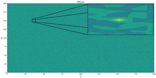
Figure 1. Atmospheric multifractal non-differentiable velocity ${\mathrm{V}}_{\mathrm{F}}\left(\mathrm{x},\mathrm{t}\right)$ plot in multifractal non-dimensional coordinates, $\mathsf{\Omega }=0.5$; zoom: peak produced by spontaneous symmetry break.

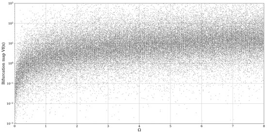
Figure 2. Bifurcation map of atmospheric multifractal non-differentiable velocity ${\mathrm{V}}_{\mathrm{F}}\left(\mathrm{x},\mathrm{t}\right)$; control parameter: $\mathsf{\Omega }$.

In order to perform the connection between the multifractal and the stochastic in a practical manner, we shall assume an application of the stochastic conservative passive additive evolution equation for ${\mathrm{V}}_{\mathrm{F}}$, considering only the non-differentiable part of the atmospheric stream, and thus arrive at an evolution equation of the assumed stochastic multifractal additive $\mathsf{\vartheta }\equiv {\mathrm{V}}_{\mathrm{F}}$ in the strictly non-differentiable part of the multifractal flow:

$$\frac{\partial ⟨{\mathrm{V}}_{\mathrm{F}}⟩}{\partial \mathrm{t}}+\nabla \left(-{\mathrm{K}}_{{\mathrm{V}}_{\mathrm{F}}}·\nabla ⟨{\mathrm{V}}_{\mathrm{F}}⟩-{\mathrm{D}}_{{\mathrm{V}}_{\mathrm{F}}}·\nabla ⟨{\mathrm{V}}_{\mathrm{F}}⟩\right)=0$$

(44)

This then, through correspondence, implies the following identities:

$${\mathrm{D}}_{{\mathrm{V}}_{\mathrm{F}}}=-\frac{\mathrm{i}}{2}\mathsf{\mu }\mathsf{\lambda }\left(\mathsf{\mu }\right)$$

(45)

$${\mathrm{K}}_{{\mathrm{V}}_{\mathrm{F}}}=-{\left(\nabla ⟨{\mathrm{V}}_{\mathrm{F}}⟩\right)}^{-1}⟨{{{\mathrm{V}}_{\mathrm{F}}}^{\prime }}^2⟩$$

(46)

$$⟨{\mathrm{N}}_{{\mathrm{V}}_{\mathrm{F}}}⟩\equiv {\mathsf{\epsilon }}_{{\mathrm{V}}_{\mathrm{F}}}\cong -\nabla ⟨{\mathrm{V}}_{\mathrm{F}}⟩⟨{{{\mathrm{V}}_{\mathrm{F}}}^{\prime }}^2⟩=-\frac{\mathrm{i}}{2}\mathsf{\mu }\mathsf{\lambda }\left(\mathsf{\mu }\right)⟨{\left(\nabla {{\mathrm{V}}_{\mathrm{F}}}^{\prime }\right)}^2⟩$$

(47)

.

Naturally, inhomogeneity variation becomes synonymous with energy dissipation once the chosen parameter is chosen to be the velocity. What also occurs is that, because of the stochastic nature of the theories, these coefficients are time-constant and each represent a value for a certain part of the system in space. Let us also note that this behavior of the coefficients occurs through time averaging, in which only the non-dimensional spatial coordinate $\mathrm{x}$ and the constant $\mathsf{\Omega }$ remains.

The multifractal Reynolds number can be deduced next using Equation (43). This results in:

$${\mathrm{Re}}_{{\mathrm{V}}_{\mathrm{F}}}=\frac{1}{3}\frac{⟨{\left(\nabla {{\mathrm{V}}_{\mathrm{F}}}^{\prime }\right)}^2⟩}{{\left(\nabla ⟨{\mathrm{V}}_{\mathrm{F}}⟩\right)}^2}$$

(48)

The Reynolds number plot presents multiple very intense peaks, and other fluctuations that greatly vary in order; however, it is safe to assume that an “average” Reynolds number, averaged thus across the entire multifractal non-differentiable velocity field, would be on the order of hundreds (Figure 3). This is also seen in Figure 4, which shows certain areas corresponding to certain values of the control parameter that exhibit very high values; yet for the majority of the map, the area would average to values in the order of hundreds. This result is reasonable, given the initial laminar nature of the modeled flow; studies have shown that turbulent Reynolds numbers are of the order of several thousands in pipe or duct flows [29,30]. Furthermore, in boundary layer flows over a flat plate, the turbulent Reynolds number is on the order of ${10}^5$ [31]. Moreover, we must highlight that the modeled non-differentiable multifractal flow is indeed an open atmospheric flow, potentially increasing the real critical turbulent Reynolds number even more. In any case, the introduction of ceilometer data will verify that, in real atmospheric turbulent cases, this number is much higher than the average of our modeled multifractal data, which is to be expected.

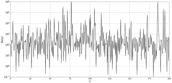
Figure 3. Reynolds number $\mathrm{Re}\left(\mathrm{x}\right)$ plot in multifractal non-dimensional coordinates, $\mathsf{\Omega }=0.5$.

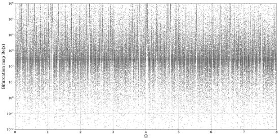
Figure 4. Bifurcation map of Reynolds number $\mathrm{Re}\left(\mathrm{x}\right)$; control parameter: $\mathsf{\Omega }$.

Observing Equation (47), it is possible to deduce that $\mathsf{\mu }$ is the only quantity that is an a priori unknown. The coefficient $\mathsf{\lambda }\left(\mathsf{\mu }\right)$ is directly connected to the coefficient $\mathsf{\Omega }$ [11]. Thus, we find that:

$$\mathsf{\mu }=-2\mathrm{i}(⟨{{{\mathrm{V}}_{\mathrm{F}}}^{\prime }}^2⟩\nabla ⟨{\mathrm{V}}_{\mathrm{F}}⟩){[⟨{\left(\nabla {{\mathrm{V}}_{\mathrm{F}}}^{\prime }\right)}^2⟩]}^{-1}$$

(49)

Through Equation (12), it is now possible to determine the singularity spectrum of the system at a given position:

$$\mathrm{f}\left(\mathsf{\alpha }\right)=\frac{2\ln \left(\mathrm{dt}\right)}{\ln \left(\mathrm{dt}\right)+\ln \{-2\mathrm{i}(⟨{{{\mathrm{V}}_{\mathrm{F}}}^{\prime }}^2⟩\nabla ⟨{\mathrm{V}}_{\mathrm{F}}⟩){[⟨{\left(\nabla {{\mathrm{V}}_{\mathrm{F}}}^{\prime }\right)}^2⟩]}^{-1}\}}$$

(50)

The dependency of this function on the scale resolution $\mathrm{dt}$ is expected, given the multifractal nature of the studied velocity field; however, despite the fact that it is necessarily an initial input parameter in the model in order to construct plots of $\mathrm{f}\left(\mathsf{\alpha }\right)$, it is unclear what $\mathrm{dt}$ values would create anomalous $\mathrm{f}\left(\mathsf{\alpha }\right)$ profiles. What is clear, however, is that certain limits must exist, otherwise $\mathrm{f}\left(\mathsf{\alpha }\right)$ could imply unreasonably high dimensions at certain scale resolutions; an aspect must be highlighted here.

In our previous studies, using a modified turbulent cascade stage model, we deduced that certain limits must exist for the initial scaling, otherwise the model would produce vortex dimensions that could be either too high or too low for typical real atmospheric flows [18,19]. Obviously, the flow modelled by the equations in this current work are not turbulent; however, it stands to reason that, just how in turbulent staging models only certain initial values are realistic, in our present case only certain scale resolutions would present valid information. Previously, when first examining such theories that can lead to the existence of atmospheric laminar channels, certain scale resolutions yielded potential amplitude fields that appeared to have a partially self-similar structure; thus, these are the scale resolutions that we shall employ [11].

For the given typical scale resolution, $\mathrm{f}\left(\mathsf{\alpha }\right)$ seems to yield dimensions roughly in the sub-unitary regime—this is to be expected from a non-differentiable component of what is necessarily a laminar flow (Figure 5 and Figure 6). Higher values of $\mathrm{f}\left(\mathsf{\alpha }\right)$, and thus of fractal dimensions, are possible with greater scale resolution; however, such larger values would imply vortex-like structures and thus partially or completely developed turbulence, which is not compatible with our initial conditions. There are many types of fractals with low, sub-unitary dimensions, such as the Feigenbaum attractor or the Cantor set; thus, the obtained results are plausible [32]. In any case, these results show that the multifractal non-differentiable velocity field presents a disjointed structure, as expected from an atmospheric multifractal flow that is initially considered laminar (Figure 5 and Figure 6). It is important to note that the superior apparent cutout seen in Figure 6 is not solid, and the maximum $\mathrm{f}\left(\mathsf{\alpha }\right)$ values do in fact decrease very slowly with $\mathsf{\Omega }$.

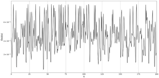
Figure 5. Singularity spectrum $\mathrm{f}\left(\mathsf{\alpha }\right)\left(\mathrm{x}\right)$ plot in multifractal non-dimensional coordinates, $\mathsf{\Omega }=0.5$.

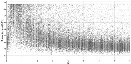
Figure 6. Bifurcation map of singularity spectrum $\mathrm{f}\left(\mathsf{\alpha }\right)\left(\mathrm{x}\right)$; control parameter: $\mathsf{\Omega }$.

In order to draw parallels between the theory and real data, it is required to introduce experimental ceilometer data. These data shall be used to calculate the initial and final turbulent scales in order for the Reynolds number profile and the atmospheric fractal dimension profile to be obtained, and for this, the structure coefficient of the refraction index profile ${\mathrm{C}}_{\mathrm{N}}^{2 }\left(\mathrm{L}\right)$ must be calculated through the following equation [18,26]:

$${ \mathsf{\sigma }}_{\mathrm{I}}^2\left(\mathrm{L}\right)=1.23{ \mathrm{C}}_{\mathrm{N}}^{2 }\left(\mathrm{L}\right){\mathrm{k}}^{\frac{7}{6}}{\mathrm{L}}^{\frac{11}{6}}$$

(51)

where ${ \mathsf{\sigma }}_{\mathrm{I}}^2$ is the “scintillation,” the logarithm of the standard deviation of light intensity of a source of light observed from a distance represented by the optical path $\mathrm{L}$. $\mathrm{I}$ refers to the intensity of the backscattered range-corrected lidar signal at the particular point in the optical path, i.e., the RCS (range corrected signal) intensity, and this can be used to calculate the scintillation [11,17,18,26]. In past studies it has been deemed and proved sufficient to employ three RCS profiles in the averaging process. After the ${\mathrm{C}}_{\mathrm{N}}^{2 }$ profile has been determined, it is now possible to calculate the length scales with a degree of approximation. The inner scale profile is linked to scintillation:

$${\mathsf{\sigma }}_{\mathrm{I}}^2\left(\mathrm{L}\right)\cong 0.615{ \mathrm{C}}_{\mathrm{N}}^{2 }\left(\mathrm{L}\right){\mathrm{L}}^3{\mathrm{l}}_{\mathrm{d}}{\left(\mathrm{L}\right)}^{\frac{-7}{3}}$$

(52)

and the outer scale can be connected to the ${\mathrm{C}}_{\mathrm{N}}^{2 }$ profile:

$${\mathrm{C}}_{\mathrm{N}}^2\left(\mathrm{z}\right)={ \mathrm{L}}_0{\left(\mathrm{z}\right)}^{\frac{4}{3}}{\left(\nabla ⟨\mathrm{n}\left(\mathrm{z}\right)⟩\right)}^2$$

(53)

For atmospheric turbulent eddies in the inertial subrange the following approximation is possible:

$$\mathrm{n}\left(\mathrm{z}\right)\cong {\mathrm{n}}_0-\sqrt{{\mathrm{C}}_{\mathrm{N}}^2\left(\mathrm{z}\right){\mathrm{z}}^{\frac{2}{3}}}$$

(54)

which can then be used to extract the outer scale profile. This method is well-referenced in our studies and has been already used successfully multiple times.

The platform used to produce ceilometer data is a CHM15k ceilometer operating at a $1064 \mathrm{nm}$ wavelength. It is positioned in Galați, Romania, at the UGAL-REXDAN facility found at coordinates $45.43 \mathrm{N}$, $28.04 \mathrm{E}$, $65 \mathrm{m}$ ASL, which is a part of the “Dunărea de Jos” University of Galați (UGAL). The instrument itself has been chosen so as to conform to the standards imposed by the ACTRIS community. From a computational perspective, the necessary calculations are performed through code written and operated in Python 3.6.

The ceilometer data have been obtained on the 22 December 2021, starting pre-noon at 11:00AM. Numerous features of the atmosphere, including clouds, aerosol plumes, and the PBL (planetary boundary layer), along with its diurnal variation, can be observed in the RCS data (Figure 6, Figure 7, Figure 8, Figure 9 and Figure 10).

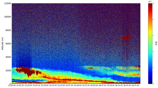
Figure 7. RCS timeseries, $\mathsf{\lambda }=1064 \mathrm{nm}$, Galați, Romania, 22 December 2021.

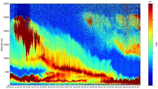
Figure 8. Zoomed-in RCS timeseries, $\mathsf{\lambda }=1064 \mathrm{nm}$, Galați, Romania, 22 December 2021.

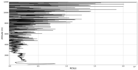
Figure 9. RCS vertical profile, $\mathsf{\lambda }=1064 \mathrm{nm}$, Galați, Romania, 22 December 2021.

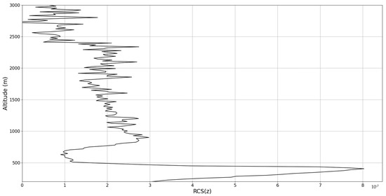
Figure 10. Zoomed-in RCS profile, $\mathsf{\lambda }=1064 \mathrm{nm}$ Galați, Romania, 22 December 2021.

The coefficient ${\mathrm{C}}_{\mathrm{N}}^{2 }$ (${\mathrm{m}}^{-\frac{2}{3}}$) is commonly used as an indicator of atmospheric turbulence strength; it can be also used to more accurately quantify the PBL altitude, and to identify regions of atmospheric calm or extreme turbulence (Figure 11, Figure 12, Figure 13 and Figure 14) [25].

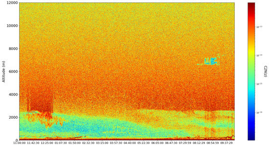
Figure 11. ${\mathrm{C}}_{\mathrm{N}}^{2 }$ timeseries, $\mathsf{\lambda }=1064 \mathrm{nm}$, Galați, Romania, 22 December 2021.

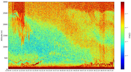
Figure 12. Zoomed-in ${\mathrm{C}}_{\mathrm{N}}^{2 }$ timeseries, $\mathsf{\lambda }=1064 \mathrm{nm}$, Galați, Romania, 22 December 2021.

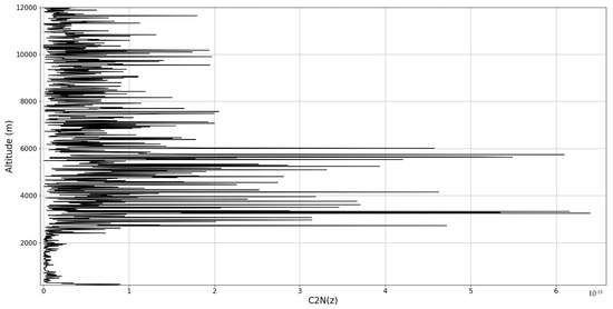
Figure 13. ${\mathrm{C}}_{\mathrm{N}}^{2 }$ profile, $\mathsf{\lambda }=1064 \mathrm{nm}$, Galați, Romania, 22 December 2021.

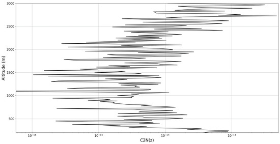
Figure 14. Zoomed-in ${\mathrm{C}}_{\mathrm{N}}^{2 }$ profile, $\mathsf{\lambda }=1064 \mathrm{nm}$, Galați, Romania, 22 December 2021.

As expected, the Reynolds number is increasing in those regions where ${\mathrm{C}}_{\mathrm{N}}^{2 }$ increases in the superior regions of the atmosphere (Figure 15, Figure 16, Figure 17 and Figure 18). Generally speaking, values appear to be between ${10}^5$ and ${10}^6$, which is in concordance to the previous discussion regarding the modelled multifractal Reynolds number. In any case, beyond what has already been discussed regarding the modelled multifractal Reynolds number, it is possible to empirically determine that the atmospheric Reynolds number should be of orders between ${10}^5$ and ${10}^6$, given the fact that the general formula is $\mathrm{Re}=\frac{\mathrm{uL}}{\mathsf{\nu }}$, where $\mathrm{u}$ is flow velocity, $\mathrm{L}$ is a characteristic dimension, and $\mathsf{\nu }$ is atmospheric kinematic viscosity, which is $1.46·{10}^{-5} \frac{{\mathrm{m}}^2}{\mathrm{s}}$ at sea level [33]. Furthermore, in that case, the high peaks produced by the spontaneous symmetry break mechanism are of the order ${10}^6$, which matches well with the experimental results.

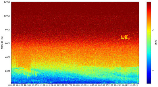
Figure 15. $\mathrm{Re}$ timeseries, $\mathsf{\lambda }=1064 \mathrm{nm}$, Galați, Romania, 22 December 2021.

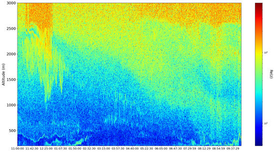
Figure 16. Zoomed-in $\mathrm{Re}$ timeseries, $\mathsf{\lambda }=1064 \mathrm{nm}$, Galați, Romania, 22 December 2021.

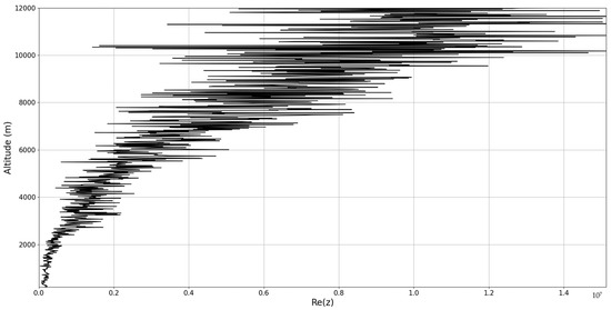
Figure 17. $\mathrm{Re}$ profile, $\mathsf{\lambda }=1064 \mathrm{nm}$, Galați, Romania, 22 December 2021.

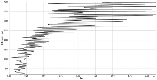
Figure 18. Zoomed-in $\mathrm{Re}$ profile, $\mathsf{\lambda }=1064 \mathrm{nm}$, Galați, Romania, 22 December 2021.

Given the fact that the minimal fractal dimension of atmospheric turbulent vortices is logically $2$, and the maximal fractal dimension of atmospheric turbulent vortices is $3$, it is quite normal for the average of these vortices, as plotted in Figure 19, Figure 20, Figure 21 and Figure 22, to be quite close to $3$ since the dimensions rapidly increase asymptotically towards $3$ in the turbulent cascade [18]. Generally speaking, this means that comparisons between the multifractal model and real data are difficult, especially considering the fact that one produces a spectrum, and the other an average of dimensions. However, a comparison can still be made regarding the evolution of the data; it is known from a previous work that $\mathsf{\Omega }~\frac{1}{\mathsf{\lambda }\left(\mathsf{\mu }\right)}$, which through Equation (45) also implies $\mathsf{\Omega }~\frac{1}{\mathrm{D}}$ [11]. This implies that low values of $\mathsf{\Omega }$ are meant to represent high laminarity, or a decreased amount of turbulence. Additionally, according to Figure 6, for the majority of the evolution of the singularity spectrum, a low $\mathsf{\Omega }$ implies a high $\mathrm{f}\left(\mathsf{\alpha }\right)$. All these facts can be combined to say that calm regions of the atmosphere are modeled to exhibit higher dimensionality, and indeed this is shown in the experimental data, where the largest values are under the PBL (Figure 19, Figure 20, Figure 21 and Figure 22).

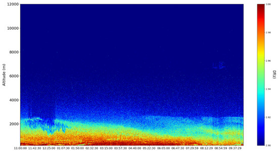
Figure 19. ${\mathrm{D}}_{\mathrm{F}}$ timeseries, $\mathsf{\lambda }=1064 \mathrm{nm}$, Galați, Romania, 22 December 2021.

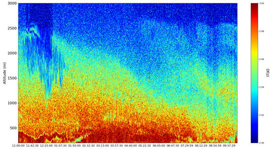
Figure 20. Zoomed-in ${\mathrm{D}}_{\mathrm{F}}$ timeseries, $\mathsf{\lambda }=1064 \mathrm{nm}$, Galați, Romania, 22 December 2021.

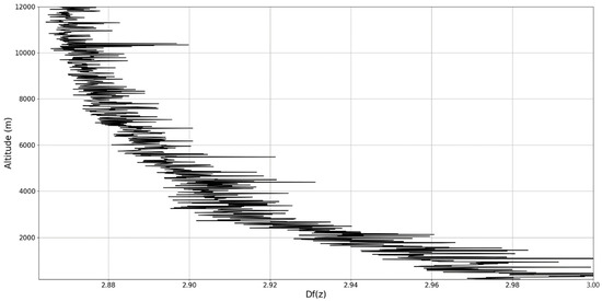
Figure 21. ${\mathrm{D}}_{\mathrm{F}}$ profile, $\mathsf{\lambda }=1064 \mathrm{nm}$, Galați, Romania, 22 December 2021.

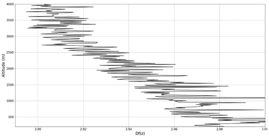
Figure 22. Zoomed-in ${\mathrm{D}}_{\mathrm{F}}$ profile, $\mathsf{\lambda }=1064 \mathrm{nm}$, Galați, Romania, 22 December 2021.

5. Conclusions

In this paper, we have found that multifractality and laminarity can be connected directly by implementing multifractal non-differentiable velocity fields into stochastic additive evolution equations. These velocity fields, having been calculated through special operational procedures on multifractal conservation equations, have been previously shown to manifest spontaneous symmetry breaks which can represent singularities that lead to turbulence generation. Starting thus from a laminar multifractal flow, it is possible to spontaneously arrive at turbulent behavior, and our analysis confirms this theory. Firstly, beyond other turbulent parameters that describe inhomogeneity dissipation or production, a multifractal Reynolds number is calculated which not only manifests typical average values for laminar flows, but also manifests strong peaks in accordance with the spontaneous symmetry breaks. Secondly, the multifractal singularity spectrum has been plotted and has been shown to reveal realistic values considering the initial conditions of the multifractal flow. These two results have been obtained strictly through correlating multifractality and stochasticity. Finally, relevant ceilometer data are presented, along with the associated theoretical background, and experimental data are found to support our theoretical developments.

From this data, and employing the model proposed here, the multifractal variational transport coefficient ${\mathrm{K}}_{{\mathrm{V}}_{\mathrm{F}}}$, the multifractal molecular diffusion coefficient ${\mathrm{D}}_{{\mathrm{V}}_{\mathrm{F}}}$, and the multifractal inhomogeneity variation $⟨{\mathrm{N}}_{{\mathrm{V}}_{\mathrm{F}}}⟩$ have been found. Overall, we found through our analysis the validity of both theories and of the connection between them, through theoretical and experimental means. Future studies will need to focus on exploiting such relationships, perhaps in determining new meteorological additives and employing multifractal theories in various approximations.

References

- Bar-Yam, Y.; McKay, S.R.; Christian, W. Dynamics of Complex Systems (Studies in Nonlinearity). Comput. Phys. 1998, 12, 335–336. [Google Scholar] [CrossRef] [Green Version]
- Mitchell, M. Complexity: A Guided Tour; Oxford University Press: Oxford, UK, 2009. [Google Scholar]
- Badii, R.; Politi, A. Complexity: Hierarchical Structures and Scaling in Physics; Cambridge University Press: Cambridge, UK, 1999; p. 6. [Google Scholar]
- Flake, G.W. The Computational Beauty of Nature: Computer Explorations of Fractals, Chaos, Complex Systems, and Adaptation; MIT Press: Cambridge, MA, USA, 1998. [Google Scholar]
- Țîmpu, S.; Sfîcă, L.; Dobri, R.V.; Cazacu, M.M.; Nita, A.I.; Birsan, M.V. Tropospheric Dust and Associated Atmospheric Circulations over the Mediterranean Region with Focus on Romania’s Territory. Atmosphere 2020, 11, 349. [Google Scholar] [CrossRef] [Green Version]
- Baleanu, D.; Diethelm, K.; Scalas, E.; Trujillo, J.J. Fractional Calculus: Models and Numerical Methods; World Scientific: Singapore, 2012; Volume 3. [Google Scholar]
- Ortigueira, M.D. Fractional Calculus for Scientists and Engineers; Springer Science & Business Media: Berlin, Germany, 2011; Volume 84. [Google Scholar]
- Nottale, L. Scale Relativity and Fractal Space-Time: A New Approach to Unifying Relativity and Quantum Mechanics; Imperial College Press: London, UK, 2011. [Google Scholar]
- Merches, I.; Agop, M. Differentiability and Fractality in Dynamics of Physical Systems; World Scientific: Singapore, 2015. [Google Scholar]
- Mandelbrot, B.B. The Fractal Geometry of Nature; WH Freeman: San Fracisco, CA, USA, 1982. [Google Scholar]
- Roșu, I.A.; Nica, D.C.; Cazacu, M.M.; Agop, M. Cellular self-structuring and turbulent behaviors in atmospheric laminar channels. Front. Earth Sci. 2022, 9, 801020. [Google Scholar] [CrossRef]
- Benzi, R.; Paladin, G.; Parisi, G.; Vulpiani, A. On the multifractal nature of fully developed turbulence and chaotic systems. J. Phys. A Math. Gen. 1984, 17, 3521. [Google Scholar] [CrossRef]
- Schertzer, D.; Lovejoy, S.; Schmitt, F.; Chigirinskaya, Y.; Marsan, D. Multifractal cascade dynamics and turbulent intermittency. Fractals 1997, 5, 427–471. [Google Scholar] [CrossRef]
- Lovejoy, S.; Schertzer, D. The Weather and Climate: Emergent Laws and Multifractal Cascades; Cambridge University Press: Cambridge, UK, 2018. [Google Scholar]
- Plocoste, T.; Carmona-Cabezas, R.; Jiménez-Hornero, F.J.; de Ravé, E.G. Background PM10 atmosphere: In the seek of a multifractal characterization using complex networks. J. Aerosol Sci. 2021, 155, 105777. [Google Scholar] [CrossRef]
- Lovejoy, S.; Schertzer, D.; Stanway, J.D. Direct evidence of multifractal atmospheric cascades from planetary scales down to 1 km. Phys. Rev. Lett. 2001, 86, 5200. [Google Scholar] [CrossRef] [PubMed] [Green Version]
- Roşu, I.A.; Cazacu, M.M.; Ghenadi, A.S.; Bibire, L.; Agop, M. On a multifractal approach of turbulent atmosphere dynamics. Front. Earth Sci. 2020, 8, 216. [Google Scholar] [CrossRef]
- Roșu, I.A.; Cazacu, M.M.; Agop, M. Multifractal Model of Atmospheric Turbulence Applied to Elastic Lidar Data. Atmosphere 2021, 12, 226. [Google Scholar] [CrossRef]
- Roșu, I.A.; Nica, D.C.; Cazacu, M.M.; Agop, M. Towards Possible Laminar Channels through Turbulent Atmospheres in a Multifractal Paradigm. Atmosphere 2021, 12, 1038. [Google Scholar] [CrossRef]
- Cristescu, C.P. Nonlinear Dynamics and Chaos. Theoretical Fundaments and Application; Romanian Academy Publishing House: Bucharest, Romania, 1987. [Google Scholar]
- Jackson, E.A. Perspectives of Nonlinear Dynamics; CUP Archive: Cambridge, UK, 1989; Volume 1. [Google Scholar]
- Nottale, L. Scale relativity and fractal space-time: Applications to quantum physics, cosmology and chaotic systems. Chaos Solitons Fractals 1996, 7, 877–938. [Google Scholar] [CrossRef]
- Agop, M.; Merches, I. Operational Procedures Describing Physical Systems; CRC Press: Boca Raton, FL, USA, 2018. [Google Scholar]
- Agop, M.; Paun, P.V. On the New Perspective of Fractal Theory. Fundaments and Applications; Editura Academiei Romane: Bucharest, Romania, 2017. [Google Scholar]
- Tatarski, V.I. Wave Propagation in a Turbulent Medium; Courier Dover Publications: Mineola, NY, USA, 2016. [Google Scholar]
- Rosu, I.A.; Cazacu, M.M.; Prelipceanu, O.S.; Agop, M. A Turbulence-Oriented Approach to Retrieve Various Atmospheric Parameters Using Advanced Lidar Data Processing Techniques. Atmosphere 2019, 10, 38. [Google Scholar] [CrossRef] [Green Version]
- Tatarski, V.I. The Effects of the Turbulent Atmosphere on Wave Propagation; Israel Program for Scientific Translations: Jerusalem, Israel, 1971. [Google Scholar]
- Oboukhov, A.M. Structure of the temperature field in turbulent flows. Isv. Geogr. Geophys. Ser. 1949, 13, 58–69. [Google Scholar]
- Schlichting, H.; Gersten, K. Boundary-Layer Theory; Springer: Berlin/Heidelberg, Germany, 2017. [Google Scholar]
- Holman, J.P. Heat Transfer (Si Units ed.); McGraw-Hill Education (India) Pvt Limited: Noida, India, 2002. [Google Scholar]
- Incropera, F.P.; DeWitt, D.P. Fundamentals of Heat Transfer; Wiley: New York, NY, USA, 1981. [Google Scholar]
- Aurell, E. On the metric properties of the Feigenbaum attractor. J. Stat. Phys. 1987, 47, 439–458. [Google Scholar] [CrossRef]
- Kerr, J.A.; Trotman-Dickenson, A.F. Handbook of Chemistry and Physics; Weast, R.C., Ed.; CRC Press: Cleveland, OH, USA, 1976. [Google Scholar]
Publisher’s Note: MDPI stays neutral with regard to jurisdictional claims in published maps and institutional affiliations. |
© 2022 by the authors. Licensee MDPI, Basel, Switzerland. This article is an open access article distributed under the terms and conditions of the Creative Commons Attribution (CC BY) license (https://creativecommons.org/licenses/by/4.0/).