Single-Sample Face Recognition Based on Shared Generative Adversarial Network

Abstract

Single-sample face recognition is a very challenging problem, where each person has only one labeled training sample. It is difficult to describe unknown facial variations. In this paper, we propose a shared generative adversarial network (SharedGAN) to expand the gallery dataset. Benefiting from the shared decoding network, SharedGAN requires only a small number of training samples. After obtaining the generated samples, we join them into a large public dataset. Then, a deep convolutional neural network is trained on the new dataset. We use the well-trained model for feature extraction. With the deep convolutional features, a simple softmax classifier is trained. Our method has been evaluated on AR, CMU-PIE, and FERET datasets. Experimental results demonstrate the effectiveness of SharedGAN and show its robustness for single sample face recognition.

1. Introduction

In recent decades, face recognition has been one of the hottest topics in the field of computer vision and pattern recognition. Many face recognition technologies have been proposed in view of various situations, among which single-sample face recognition is a very challenging problem. In many practical applications, such as access control, passport identification, judicial confirmation, etc., only a single sample per person (SSPP) is enrolled in the gallery dataset for training. When the probe sample is affected by factors such as illumination, expression, and occlusion, the single-sample face recognition task becomes more difficult. Traditional face recognition methods [1,2,3] usually assume that each person has multiple training samples. These methods will face serious performance degradation when dealing with the single-sample face recognition task.

The biggest obstacle to solving the problem of single-sample face recognition is that the gallery dataset does not contain face variations. The existing solutions can be classified into roughly four categories: (1) methods based on local region division, (2) methods based on virtual sample generation, (3) methods based on the generic dataset, and (4) methods based on deep learning. The methods [4,5,6] based on local region division can alleviate the impact of face variations to a certain extent. However, they still cannot avoid the problem of a lack of variation information. Methods [7,8,9] based on virtual sample generation can deal with an insufficient number of training samples. They generate virtual samples, depending only on gallery samples. Therefore, there is a high correlation among the generated samples, and the variation information introduced into the generated samples is not enough. The methods [10,11,12] based on the generic dataset usually assume that face images have similar intra-class variations. They collect an additional generic dataset, in which each class has multiple face images, covering the most predictable variations. Benefiting from the external variation information, these methods significantly boost the performance of single-sample face recognition. However, it is difficult to obtain a generic dataset in practical applications. The methods [13,14,15] based on deep learning usually train the model on a large public dataset. Their performance is dependent on whether the public training dataset contains specific variations appearing in the probe samples. Therefore, they face the same problem as methods based on the generic dataset.

The existing methods, based on virtual sample generation, can increase the number of training samples, but they cannot generate samples with specific variations. The generic dataset-based methods benefit from the external variation information, but they usually use the intensity of the pixels as the features. The advantage of the deep learning-based methods lies in feature extraction, but they are restricted by specific variations. Considering the above three points, in this paper, we propose a novel scheme to fulfill the task of single-sample face recognition. Our method consists of the following main three parts:

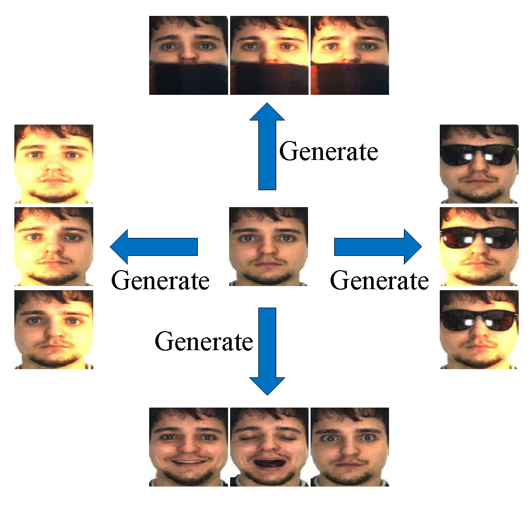
• We propose a shared generative adversarial network (SharedGAN) to expand the gallery dataset. SharedGAN is trained on the generic dataset and copies the variations in the generic dataset into the gallery samples. Compared with the methods [7,8,9], the proposed SharedGAN introduces enough variation information into the generated samples. Regarding the difficulty of collecting the generic dataset, the proposed SharedGAN requires only a small number of training samples.
• We add the generated samples and the generic dataset to a large public dataset, and then we train a deep convolutional neural network on the new dataset. We use the well-trained model for feature extraction.
• We propose a simple classification method and employ the features of the gallery and generated samples to train the classification model. Then, we classify the probe samples. Experiments on three public face databases are performed to demonstrate the effectiveness of our method.

The rest of this paper is organized as follows. In Section 2, we introduce the related work. In Section 3, we present the details of SharedGAN. In Section 4, we describe the proposed classification method. Section 5 presents the experimental results and discussion. We conclude the paper in Section 6.

2. Related Work

In this section, we first review some classical and state-of-the-art methods for handling single-sample face recognition. Then, we review the generative adversarial networks and image-to-image translation.

2.1. Single Sample Face Recognition

For the methods based on local region division, each face image is divided into a collection of local patches. According to the means of treating local regions, the methods can be divided into two categories. The methods in the first category perform recognition for each region, such as patch-based sparse representation for classification (PSRC) [3], patch-based collaborative representation for classification (PCRC) [16], and local structure-based sparse representation classification (LS-SRC) [5]. They predict the image label based on majority voting. Therefore, these methods can alleviate the effect of facial variations. The methods in the second category treat local patches of the gallery image as a training sample of this class, such as block-based Fisher linear discriminative analysis (BlockFLDA) [17], discriminative multi-manifold analysis (DMMA) [4], sparse discriminative multi-manifold embedding (SDMME) [18], and robust heterogeneous discriminative analysis (RHDA) [6]. They treat each person as a manifold and formulate face recognition as a multi-manifold matching problem. These methods only work well when the probe image contains less variation.

For methods based on virtual sample generation, data redundancy is a concerning problem. In [7,8], the authors generated multiple samples for each person by applying a singular value decomposition-based perturbation, respectively. In [9], Chu et al. divided the face into two halves according to the axis of symmetry and mirrored the right half of the face to the left, so as to expand the gallery dataset. After obtaining the virtual samples, they conducted a discriminant analysis for feature extraction. The virtual samples generated by these methods are very similar to the gallery samples. Therefore, they cannot be regarded as independent samples. In [19], Deng et al. proposed two 3D generic elastic models to synthesize faces under different poses and illumination conditions. In [20], Tu et al. first recovered the shapes and albedos of the gallery samples using a 3D face modeling module and then performed image generation by varying pose, illumination, and expression. The sample generation methods based on the 3D model are adept at introducing pose variations. They can avoid data redundancy.

For methods based on the generic dataset, there are two ways of using the generic dataset. One way is to infer the variation information from the generic dataset and introduce it to the gallery dataset, such as adaptive generic learning (AGL) [21], sparse variation dictionary learning (SVDL) [22], and collaborative probabilistic labels (CPL) [23]. The other way is to utilize the generic dataset to build the intra-class variation dictionary, which is based on the assumption that a probe sample equals its prototype plus intra-class variation (P+V) [24], such as extended sparse representation for classification (ESRC) [10], linear regression analysis with generic learning (LRA-GL) [25], local generic representation (LGR) [11], and synergistic generic learning (SGL) [26]. Thanks to the help of the generic dataset, these methods can cope with the large variation between the gallery and probe images. Consequently, they usually outperform methods that do not employ the generic dataset.

For the methods based on deep learning, the effectiveness and robustness of feature extraction affect the recognition performance. Due to the constraints of the single-sample condition, deep neural networks are usually trained on a large public dataset instead of the gallery dataset. With the well-trained model, feature extraction is performed for the gallery and probe images. Then, some classification techniques are applied. In the SGL [26] method, Pang et al. used the deep convolutional features. In [27], Yang et al. fulfilled the single-sample face recognition task by combining the (P + V) model with deep convolutional features. In [14], Min et al. proposed a k-class feature transfer (KCFT) algorithm, which enriched the intra-class variation information for the gallery face feature. Similar to the KCFT algorithm, Ding et al. [15] generated features for the gallery dataset using the conditional generative adversarial network (CGAN). Due to the strong fusion ability of deep learning, methods based on this are being developed.

2.2. Generative Adversarial Networks

Since the generative adversarial network (GAN) was proposed, scholars have applied it to different tasks, such as image generation [28,29], image synthesis [30,31], image colorization [32,33], super-resolution [34,35], and image translation [36,37]. The classical GAN model consists of two modules: a discriminator and a generator. In the training process, the discriminator’s task is to judge whether the input data are real or generated, and the task of the generator is to generate false data, which are used to cheat the discriminator so that it cannot distinguish whether the input data are real or generated. This principle is shown in Figure 1.

The objective function of GAN is as follows:

$${\mathcal{L}}_{GAN}=-{\mathbb{E}}_{x_{real}}\left[log\left(D\left(x_{real}\right)\right)\right]-{\mathbb{E}}_{x_{fake}}\left[log\left(1-D\left(x_{fake}\right)\right)\right],$$

(1)

where $\mathbb{E}$ is the mathematical expectation, D is the discriminator, $x_{real}$ is the sampled real data, and $x_{fake}$ is the data generated by the generator G. $x_{fake}=G\left(z\right)$, where z is the data that satisfy a certain distribution. The G generator tries to maximize the above formula, while the discriminator D tries to minimize it.

2.3. Image-to-Image Translation

Among the many tasks in applying GAN, the purpose of image-to-image translation is to translate images from the source domain to the target domain. Some recent work has yielded impressive results. Usually, paired samples need to be collected in both source and target domains. For example, pix2pix [38] combines conditional adversarial loss [39] and $L1$ loss, and uses paired samples for supervised learning. Based on pix2pix, Wang et al. [30] proposed a coarse-to-fine generator and a multi-scale discriminator architecture to realize high-resolution image generation. These models do not work when the paired samples are difficult to obtain. To solve this problem, unpaired image-to-image translation models have been proposed, such as CycleGAN [40], DiscoGAN [41], DualGAN [42] and UNIT [43]. An important problem is how to preserve the key content and attributes in the process of image translation. These models respond by using the cycle consistency loss as a constraint. However, the disadvantage of these models is that they can only learn the relationship between two different domains. When there are multiple domains, these models need to be trained for each pair of domains. To realize multi-domain image-to-image translation, StarGAN [36], Augmented CycleGAN [44], and MUNIT [45] are proposed. Cycle consistency loss can ensure that the translated image retains enough background information. However, in some cases, such as gender conversion, retaining too much background information will make the translated image look uncomfortable. Therefore, in order to solve this problem, Zhao et al. proposed ACL-GAN [46]. They adopted adversarial consistency loss instead of cycle consistency loss; that is, when the translated image is translated back, it only needs to maintain similarity rather than consistency. The above-mentioned GAN models require a lot of samples during training, and the performance degrades when there are only a small number of samples.

3. Shared Generative Adversarial Network

The general image-to-image translation model requires a lot of samples during training. When there is only a small number of samples, the discriminator is prone to overfitting, resulting in declines in image quality. To alleviate overfitting and obtain generated images of a higher quality, we propose a shared generative adversarial network (SharedGAN). The purpose of SharedGAN is to copy the variations in a small number of training samples into the gallery samples, so as to expand the gallery dataset. The intention of SharedGAN is shown in Figure 2. The framework of SharedGAN is shown in Figure 3.

3.1. Network Architecture

SharedGAN combines the multi-domain image-to-image translation model with the image generation model. It improves the quality of the output image of the image translation model by sharing the decoding network of the generators of the two models. The architecture of the generator of SharedGAN is shown in Figure 4, where (a) is the encoding network, (c) is the shared decoding network, (a) + (c) is the image translation network, and (b) + (c) is the image generation network. The image translation model has only a small number of samples, and its task is to translate images from the source domain to the target domain. The image generation model has a large number of samples, and its task is to generate images from data that satisfy Gaussian distribution. Using only a small number of samples, the network (a) + (c) cannot obtain robust parameters through training. If the decoding ability of the network (c) is improved, it can be predicted that the quality of the output image of the network (a) + (c) will also be improved. The proposed SharedGAN in this paper improves the decoding ability of the shared network (c) by training the network (b) + (c) with a large number of samples, and meanwhile ensures that the network (a) + (c) can fit its few training samples. In this way, the shared network (c) can learn the decoding commonality, which indirectly improves the robustness of the network (a) + (c). The architectures of the discriminators of SharedGAN are shown in Figure 5, where (d) is the shared discriminator 1 and (e) is the discriminator 2. Discriminator 1 needs to accomplish three tasks: (1) estimate the variation type of the input image, (2) judge the authenticity of the image, and (3) confirm the source of the image. Discriminator 2 only needs to accomplish one task: (4) determine whether the two input images belong to the same class. The image translation model corresponds to discriminator 1 and discriminator 2; it needs to accomplish all four tasks. The image generation model corresponds to discriminator 1; it needs to accomplish the two tasks of (2) and (3).

3.2. Multi-Domain Image-to-Image Translation Model

Suppose the training dataset is $x=\left\{\left(x_0,x_v\right)\right\}$, where $x_0$ is the prototype sample, and $x_v$ is a sample with variation v of the same class as $x_0$. For the multi-domain image-to-image translation model, we treat each variation type v of face image as a domain and denote $v_0$ as the domain of the prototype samples. Our goal is to train a generator G that adds variation v to the input image $x_0$. To improve the robustness of the translation model, we also remove variation v from the input image $x_v$. We denote the action label as c, where $c=01$ means adding variation, and $c=10$ means removing variation. The translation process can be expressed as $G\left(x,v,c\right)\to y$, where y is the output image, and $\left(v,c\right)$ is the operation performed. There are two discriminators, namely $D_1=\left\{D_{Ra},D_{var},D_{ind}\right\}$ and $D_2=\left\{D_{pis}\right\}$, where $D_{Ra}$ is a relativistic average discriminator (RaD) [47], $D_{var}$ is used to estimate the type of image variation, $D_{ind}$ is used to confirm the source of the image, and $D_{pis}$ is used to evaluate whether two images belong to the same class.

To make the generated image indistinguishable from the real image, we use the relativistic average discriminator $D_{Ra}$. The objective functions are as follows:

$${\mathcal{L}}_{Ra\_D}=-{\mathbb{E}}_x\left[log\left(D_{Ra}\left(x\right)\right)\right]-{\mathbb{E}}_{x,v,c}\left[log\left(1-D_{Ra}\left(G\left(x,v,c\right)\right)\right)\right],$$

(2)

and

$${\mathcal{L}}_{Ra\_G}=-{\mathbb{E}}_{x,v,c}\left[log\left(D_{Ra}\left(G\left(x,v,c\right)\right)\right)\right]-{\mathbb{E}}_x\left[log\left(1-D_{Ra}\left(x\right)\right)\right],$$

(3)

where

$$D_{Ra}\left(x\right)=sigmoid\left(H\left(x\right)-{\mathbb{E}}_{x,v,c}\left[H\left(G\left(x,v,c\right)\right)\right]\right),$$

(4)

$$D_{Ra}\left(G\left(x,v,c\right)\right)=sigmoid\left(H\left(G\left(x,v,c\right)\right)-{\mathbb{E}}_x\left[H\left(x\right)\right]\right),$$

(5)

$H\left(·\right)$ refers to the output of the non-transformed layer. Minimizing the loss ${\mathcal{L}}_{Ra\_D}$ can maximize the probability that the real image provided is more real than the generated image. Minimizing the loss ${\mathcal{L}}_{Ra\_G}$ can maximize the probability that the generated image is more real than the real image. We adopt PatchGANs [38] for $D_{Ra}$, which evaluates whether local image patches are real or fake.

By minimizing the above adversarial loss, the generated image can be as close to reality as possible, but the consistency of image content cannot be guaranteed. If there are very similar face images in the training dataset, the class of the generated image may change. Therefore, to ensure that the input image and the output image belong to the same class, we apply a cycle consistency loss to the generator, which is defined as follows:

$${\mathcal{L}}_{cyc}={\mathbb{E}}_{x,v,c}\left[{∥x-G\left(G\left(x,v,c\right),v,1-c\right)∥}_1\right],$$

(6)

where $1-c$ represents the reverse action of c.

Due to the difference between the distribution of data used in the image translation model and that of data used in the image generation model, it will be difficult to train the parameters if the decoding network (c) is directly shared. Therefore, we apply the image source indicator t to help the network fitting, where $t=01$ means that the data come from the image translation model, and $t=10$ means that the data comes from the image generation model. Then we add an auxiliary classifier $D_{ind}$ on the top of the discriminator network to identify the source of the image. For the image translation model, the indicator loss is as follows:

$${\mathcal{L}}_{ind}=-{\mathbb{E}}_{x,t}\left[log\left(D_{ind}\left(t=01|x\right)\right)\right]-{\mathbb{E}}_{x,v,c,t}\left[log\left(D_{ind}\left(t=01|G\left(x,v,c\right)\right)\right)\right].$$

(7)

Minimizing the above formula means that the real image and the generated image come from the same distribution.

Since the decoding network (c) is a shared network, the image generation model has a great influence on it, and the number of samples used in the image translation model is much lower than that used in the image generation model. To further guarantee the fitting of the image translation model, we add the following paired adversarial loss:

$${\mathcal{L}}_{pis}=-{\mathbb{E}}_{x_0,x_v}\left[log\left(D_{pis}\left(x_0,x_v\right)\right)\right]-{\mathbb{E}}_{x,v,c}\left[log\left(1-D_{pis}\left(x,G\left(x,v,c\right)\right)\right)\right],$$

(8)

where $D_{pis}$ is used to evaluate whether two images belong to the same class.

For the input image $x_0$ and the operation $(v,c=01)$, our goal is to translate $x_0$ into the output image y, which has variation v. For the input image $x_v$ and the operation $(v,c=10)$, our goal is to eliminate variation v in the image $x_v$. To achieve this, we add an auxiliary classifier $D_{var}$ on the top of the discriminator network to distinguish the images’ variation types. When training the discriminator network, the classification loss is as follows:

$${\mathcal{L}}_{var}^r=-{\mathbb{E}}_{x,v}\left[log\left(D_{var}\left(v|x\right)\right)\right],$$

(9)

Minimizing the above formula means that the discriminator network can classify the real image x into the variation type v. When training the generator network, the classification loss is as follows:

$${\mathcal{L}}_{var}^f=-{\mathbb{E}}_{x,v,c}\left[log\left(D_{var}\left(v|G\left(x_0,v,c=01\right)\right)\right)\right]-{\mathbb{E}}_{x,v,c}\left[log\left(D_{var}\left(v_0|G\left(x_v,v,c=10\right)\right)\right)\right],$$

(10)

where the first item indicates that the image generated by the image $x_0$ after adding the variation v should be correctly classified into domain v, and the second item indicates that the image generated by the paired image $x_v$ after removing the variation v should be classified into domain $v_0$.

In many cases, a lot of background information can be retained on the input image. We hope that the generated image can be modified from the source image; that is, only modifying certain areas of the source image and keeping the rest unchanged. We cause the generator to produce four channels, where the first three are the channels of RGB image $x_t$, and the fourth is called a bounded focus mask $x_m$. The values of $x_m$ are between 0 and 1. The final output image can be represented by the following formula:

$$x_{out}=x+\left(x_t-x\right) \odot x_m,$$

(11)

where ⊙ is element-wise product. For the mask $x_m$, we add the following constraint:

$${\mathcal{L}}_{mask}={\left(\frac{1}{W}\sum _k|x_m\left[k\right]|\right)}^2,$$

(12)

where $x_m\left[k\right]$ is the k-th pixel of $x_m$, and W is the number of pixels. The above formula encourages the reduction of changes to the source image.

Based on the above discussion, the total loss of the image translation model is as follows:

$${\mathcal{L}}_D={\mathcal{L}}_{Ra\_D}+{\lambda }_{pis}{\mathcal{L}}_{pis}+{\lambda }_{var}{\mathcal{L}}_{var}^r+{\lambda }_{ind}{\mathcal{L}}_{ind},$$

(13)

$${\mathcal{L}}_G={\mathcal{L}}_{Ra\_G}-{\lambda }_{pis}{\mathcal{L}}_{pis}+{\lambda }_{cyc}{\mathcal{L}}_{cyc}+{\lambda }_{var}{\mathcal{L}}_{var}^f+{\lambda }_{ind}{\mathcal{L}}_{ind}+{\lambda }_{mask}{\mathcal{L}}_{mask},$$

(14)

where ${\lambda }_{pis}$, ${\lambda }_{var}$, ${\lambda }_{ind}$, ${\lambda }_{cyc}$, and ${\lambda }_{mask}$ are hyper-parameters that control the relative importance of each item.

3.3. Image Generation Model

For the image generation model, the input is 100 dimensional random data $z\sim N\left(0,1\right)$. Our goal is to train a generator $G^{†}$ to translate z into an output image $x_t$, which is composed of the first three channels of the output of the network (c). The process can be expressed as $G^{†}\left(z\right)\to x_t$. The discriminator is $D_1=\left\{D_{Ra},D_{ind}\right\}$ that is shared with the image translation model. We adopt the relativistic average discriminator $D_{Ra}$; the objective functions are as follows:

$${\mathcal{L}}_{D\_Ra}^{†}=-{\mathbb{E}}_x\left[log\left(D_{Ra}\left(x\right)\right)\right]-{\mathbb{E}}_z\left[log\left(1-D_{Ra}\left(G^{†}\left(z\right)\right)\right)\right],$$

(15)

and

$${\mathcal{L}}_{G\_Ra}^{†}=-{\mathbb{E}}_z\left[log\left(D_{Ra}\left(G^{†}\left(z\right)\right)\right)\right]-{\mathbb{E}}_x\left[log\left(1-D_{Ra}\left(x\right)\right)\right],$$

(16)

where

$$D_{Ra}\left(x\right)=sigmoid\left(H\left(x\right)-{\mathbb{E}}_z\left[H\left(G^{†}\left(z\right)\right)\right]\right),$$

(17)

$$D_{Ra}\left(G^{†}\left(z\right)\right)=sigmoid\left(H\left(G^{†}\left(z\right)\right)-{\mathbb{E}}_x\left[H\left(x\right)\right]\right),$$

(18)

where $H\left(·\right)$ refers to the output of the non-transformed layer.

As for the image source, the data corresponding to the image generation model and its generated images should be classified into $t=10$. The classification loss is as follows:

$${\mathcal{L}}_{ind}^{†}=-{\mathbb{E}}_{x,t}\left[log\left(D_{ind}\left(t=10|x\right)\right)\right]-{\mathbb{E}}_{z,t}\left[log\left(D_{ind}\left(t=10|G^{†}\left(z\right)\right)\right)\right].$$

(19)

Based on the above discussion, the total loss of the image generation model is as follows:

$${\mathcal{L}}_D^{†}={\lambda }_{Ra}{\mathcal{L}}_{Ra\_D}^{†}+{\lambda }_{ind}^{†}{\mathcal{L}}_{ind}^{†},$$

(20)

$${\mathcal{L}}_G^{†}={\lambda }_{Ra}{\mathcal{L}}_{Ra\_G}^{†}+{\lambda }_{ind}^{†}{\mathcal{L}}_{ind}^{†},$$

(21)

where ${\lambda }_{Ra}$ and ${\lambda }_{ind}^{†}$ are hyper-parameters that control the relative importance of each item. The parameter ${\lambda }_{Ra}$ is added because the influence of the training of the image generation model on the network (c) needs to be adjusted.

4. Classification Method

After obtaining the generated samples, we add them and the generic dataset to a large public dataset, and then we train a deep convolutional neural network on the new dataset. With the well-trained model, feature extraction is performed. The extracted features have been mapped to the hypersphere feature space by $L2$ normalization. We train a softmax classifier with deep convolutional features. The features of the gallery, generated, and generic samples are denoted by x, $\overline{x}$, and $\widehat{x}$, respectively. As usual, x and $\overline{x}$ are mapped to the class that they belong to. For the softmax classifier, $\widehat{x}$ does not belong to any of these categories. To make the mapping matrix more robust, samples of the same class in the generic dataset are mapped to the near places, i.e.,

$$W^T{\widehat{x}}_v\approx W^T{\widehat{x}}_0,$$

(22)

where W is the mapping matrix, ${\widehat{x}}_0$ is the prototype sample, and ${\widehat{x}}_v$ is the sample with variation v of the same class as ${\widehat{x}}_0$. For Equation (22), we can make the following inference:

$$W^T{\widehat{x}}_v\approx W^T{\widehat{x}}_0\Rightarrow ∥W_k∥∥{\widehat{x}}_v∥cos{\widehat{\theta }}_{k,v}\approx ∥W_k∥∥{\widehat{x}}_0∥cos{\widehat{\theta }}_{k,0},\forall k\Rightarrow cos{\widehat{\theta }}_v\approx cos{\widehat{\theta }}_0,$$

(23)

where $W_k$ is the mapping vector of class k, ${\widehat{\theta }}_v$ is the vector of angle between W and ${\widehat{x}}_v$, and ${\widehat{\theta }}_0$ is the vector of angle between W and ${\widehat{x}}_0$.

In summary, the objective function is as follows:

$$\mathcal{L}=-\frac{1}{n}\sum _{i=1}^{n}log\frac{e^{W_{y_i}^T{x}_i}}{{\sum }_{j=1}^c{e}^{W_j^T{x}_i}}-\frac{{\alpha }_1}{m}\sum _{i=1}^{m}log\frac{e^{W_{{\overline{y}}_i}^T{\overline{x}}_i}}{{\sum }_{j=1}^c{e}^{W_j^T{\overline{x}}_i}}+\frac{{\alpha }_2}{h}\sum _{v=1}^V\sum _{q=1}^Q{∥cos{\widehat{\theta }}_{q,v}-cos{\widehat{\theta }}_{q,0}∥}_2,$$

(24)

where ${\alpha }_1$ and ${\alpha }_2$ are the weighting parameters, $y_i$ is the label of $x_i$, ${\overline{y}}_i$ is the label of ${\overline{x}}_i$, V is the number of the types of variation, Q is the number of the subjects in the generic dataset, and $h=VQ$.

5. Experimental Results and Discussion

In this section, we evaluate the proposed SharedGAN and classification method on the AR [48], CMU-PIE [49], and FERET [50] datasets.

The AR dataset contains more than 4000 color face images of 126 people (70 men and 56 women). For each person, 26 images were taken in two sessions, 13 in each session. These images had different facial variations, including different facial expressions (neutral, smile, anger, and scream), lighting conditions (light on the left, light on the right, and lights on both sides), and occlusions (sunglass and scarf). The dataset was cropped and aligned, and the image size was $120\times 165$. Figure 6 shows some sample images from the AR dataset. Similar to the works in [10,11], we carried out experiments with a subset of 100 subjects (50 men and 50 women). Eighty subjects of the first 40 men and 40 women were used as the gallery and probe datasets. The remaining 20 subjects were used as the generic dataset.

The CMU pose, illumination, and expression (CMU-PIE) dataset contains more than 40,000 facial images corresponding to 68 subjects. For each subject, the images were taken across 13 different poses, under 43 different illumination conditions, and with four different expressions. Each image was a $64\times 64$ grayscale image. We carried out experiments with five poses, i.e., C05 (looking left), C07 (looking up), C09 (looking down), C27 (looking forward), and C29 (looking right). We showed some sample images in Figure 7. The first 48 subjects were used as the gallery and probe datasets. The remaining 20 subjects were used as the generic dataset.

The FERET dataset contained 13,539 facial images of 1565 individuals. We carried out experiments with a subset that includes 1400 images from 200 individuals, which are cropped to $80\times 80$. Each individual had 7 images taken under different poses, expressions, and illumination conditions. The first 60 subjects were used as the generic dataset, while the remaining 140 subjects were used as the gallery and probe datasets. Figure 8 shows some sample images.

5.1. Evaluation for SharedGAN

The multi-domain image-to-image translation model was trained on the generic dataset, and the image generation model was trained on CelebA-HQ [51] dataset, which contains 30,000 high-quality images. The images from CelebA-HQ dataset were aligned with MTCNN [52] model. The two models of SharedGAN were alternately trained using Adam [53] with ${\beta }_1=0.5$ and ${\beta }_2=0.999$. The learning rate was set to 0.0001. The batch size was set to 20 for the multi-domain image-to-image translation model and 50 for the image generation model. All the images were resized to $128\times 128$. Training took about four hours on a single NVIDIA Tesla V100 GPU. The model size was 158.05 M. CycleGAN [44], StarGAN [36], and CUT [54] were the compared methods. We used Frechet Inception Distance (FID) [55] to evaluate the image quality, which calculates the Frechet distance with mean and covariance between the real and the fake image distributions.

5.1.1. Experiments on AR Dataset

The AR dataset contains 12 types of variation, denoted by V01-V12, as shown in Figure 6. In the experiment, we set ${\lambda }_{var}=0.5$, ${\lambda }_{pis}=0.2$, ${\lambda }_{ind}=0.1$, ${\lambda }_{cyc}=10$, and ${\lambda }_{mask}=0.5$ for the multi-domain image-to-image translation model, and we set ${\lambda }_{Ra}=0.5$ and ${\lambda }_{ind}^{†}=0.1$ for the image generation model. The generic dataset including 20 subjects was used to train SharedGAN. The neutral sample was used as the prototype sample. For two sessions, there were 40 pairs of training samples for each type of variation. Unfortunately, we can see from Figure 6 that the samples in the two sessions were very similar. Nevertheless, the proposed SharedGAN generated high-quality images, which are shown in Figure 9. The FIDs are listed in

Table 1. FID on AR Dataset.

Method	V01	V02	V03	V04	V05	V06
CycleGAN	44.4	36.4	51.5	39.2	45.6	52.7
StarGAN	91.1	89.1	115.0	83.9	81.5	102.4
CUT	34.6	32.9	46.7	33.5	32.2	48.9
SharedGAN	65.6	62.1	73.0	61.2	62.2	73.0
Method	V07	V08	V09	V10	V11	V12
CycleGAN	58.1	206.0	62.8	70.0	205.3	186.7
StarGAN	69.3	178.0	74.7	90.5	219.1	206.5
CUT	31.1	182.5	32.5	27.9	164.0	148.8
SharedGAN	45.0	130.8	42.0	37.4	161.5	141.6

, from which we can see that, in the V08, V11, and V12 items, our method achieved the best results. For StarGAN, the generated images looked blurry. For CycleGAN, in the V02 and V03 items, it failed to generate the expressions of anger and scream. For the other types of variation, the images generated by CycleGAN contained noise. Compared with CycleGAN and StarGAN, the results generated by our method look more real. For CUT, in the V02 item, it failed to generate the expression of anger, and in the V03 item, the generated image looks blurry. We also show the images generated by the image generation model of SharedGAN in Figure 10. It can be seen that the style of the generated images is similar to that of CelebA-HQ.

To verify the role of the network (b) + (c), we carried out an experiment where we only used the multi-domain image-to-image translation model to generate images, i.e., the generator is the network (a) + (c). The FIDs are listed in

Table 2. FID on AR Dataset.

Method	V01	V02	V03	V04	V05	V06
Network (a) + (c)	65.3	76.6	78.7	69.5	66.1	107.1
SharedGAN	65.6	62.1	73.0	61.2	62.2	73.0
Method	V07	V08	V09	V10	V11	V12
Network (a) + (c)	47.9	149.0	51.0	52.2	182.7	169.0
SharedGAN	45.0	130.8	42.0	37.4	161.5	141.6

. The generated images are shown in Figure 11. The original images are in the first row, and SharedGAN generates images in the second row. The multi-domain image-to-image translation model generates images in the third row. It can be seen that the network (a) + (c) generates blurry images. As a combination of the multi-domain image-to-image translation model and the image generation model, SharedGAN generates images with a higher quality than the multi-domain image-to-image translation model.

5.1.2. Experiments on CMU-PIE Dataset

The generic dataset including 20 subjects was used to train SharedGAN. The 4th, 7th, 9th, 12th, 13th, 16th, 18th, and 23rd images from C05, C07, C09, C27, and C29 were selected for the experiment. We denoted the types of variation by V01–V08, as shown in Figure 7. The 13th image from C27 was used as the prototype sample. There were 39 types of variation. For each type of variation, there were 20 pairs of training samples. In the experiment, we set ${\lambda }_{var}=1$, ${\lambda }_{pis}=0.1$, ${\lambda }_{ind}=0.1$, ${\lambda }_{cyc}=10$, and ${\lambda }_{mask}=0.03$ for the multi-domain image-to-image translation model, and we set ${\lambda }_{Ra}=0.3$ and ${\lambda }_{ind}^{†}=0.1$ for the image generation model. The generated images under the five poses are shown in Figure 12, Figure 13, Figure 14, Figure 15 and Figure 16, respectively. We can see that the visual effect is not obvious because the image resolution is poor. We show the FIDs in

Table 3. FID on CMU-PIE Dataset.

Pose	Method	V01	V02	V03	V04	V05	V06	V07	V08
C05	CycleGAN	101.5	66.3	75.5	63.6	75.3	57.1	69.7	70.9
	StarGAN	248.7	125.1	107.8	139.0	105.4	111.5	127.5	197.9
	CUT	83.8	67.7	49.7	85.1	71.2	47.2	43.6	55.9
	SharedGAN	77.2	42.9	45.0	49.7	40.6	40.0	49.6	71.9
C07	CycleGAN	69.8	56.6	79.8	61.1	59.6	52.7	54.8	64.8
	StarGAN	187.5	104.7	112.3	110.4	108.8	115.7	112.3	119.4
	CUT	68.0	54.7	45.4	58.5	51.2	40.9	38.4	53.0
	SharedGAN	78.3	43.6	49.8	47.7	44.8	43.2	51.0	71.6
C09	CycleGAN	121.9	68.1	74.4	69.0	64.5	54.7	59.1	72.8
	StarGAN	216.3	140.8	137.4	148.8	147.4	148.2	159.9	251.7
	CUT	95.8	45.9	46.4	46.4	62.9	46.1	48.6	57.0
	SharedGAN	99.3	58.9	52.6	62.0	63.1	57.0	62.7	113.9
C27	CycleGAN	66.7	75.0	44.9	52.9	-	47.3	53.4	63.7
	StarGAN	142.8	78.6	78.3	85.2	-	71.9	85.6	157.7
	CUT	57.1	45.8	40.3	49.7	-	35.9	34.8	50.5
	SharedGAN	63.4	39.3	52.3	38.4	-	35.8	38.9	62.6
C29	CycleGAN	89.1	70.2	70.9	83.3	68.4	67.2	62.8	83.6
	StarGAN	263.6	141.4	132.6	152.1	129.3	112.7	122.4	234.1
	CUT	95.5	62.0	77.2	74.9	51.6	75.6	75.2	75.6
	SharedGAN	100.0	60.7	57.4	68.9	52.0	53.1	71.6	117.5

. It can be seen that our method achieved the best results in many cases.

5.1.3. Experiments on FERET Dataset

The generic dataset including 60 subjects was used to train SharedGAN. As shown in Figure 8, the neutral sample was used as the prototype sample. The six types of variation were denoted by V01-V06. For each type of variation, there were 60 pairs of training samples. In the experiment, we set ${\lambda }_{var}=0.5$, ${\lambda }_{pis}=0.5$, ${\lambda }_{ind}=0.1$, ${\lambda }_{cyc}=10$, and ${\lambda }_{mask}=0.01$ for the multi-domain image-to-image translation model, and we set ${\lambda }_{Ra}=0.5$ and ${\lambda }_{ind}^{†}=0.1$ for the image generation model. The generated images are shown in Figure 17, from which we can see that the images generated by StarGAN are blurry. For CycleGAN, this failed to generate the images in the V01 and V04 items. For CUT, it failed to generate the images in the V01, V02, V03, and V04 items. Using our method, the quality of the generated images was not as good as that of the images generated on the AR dataset. This could be because a large difference exists in terms of data distribution between the samples used to train the multi-domain image-to-image translation model and the samples used to train the image generation model. We list the FIDs in

Table 4. FID on FERET Dataset.

Method	V01	V02	V03	V04	V05	V06
CycleGAN	48.4	40.8	35.4	47.1	32.8	57.1
StarGAN	128.4	118.0	123.8	131.2	131.3	181.4
CUT	43.2	46.8	40.5	50.6	44.2	42.1
SharedGAN	48.4	48.7	47.4	49.0	44.7	73.8

. It can be seen that CycleGAN achieved the best results. However, the images generated by CycleGAN look unnatural.

5.2. Evaluation for Single Sample Face Recognition

We used the inception-resnet-v2 [56] model as the deep convolutional neural network architecture. The objective function is a softmax loss plus a center loss [57]. The model was trained on the dataset consisting of CASIA-WebFace [58] dataset, generated samples, and the generic dataset. The samples from CASIA-WebFace dataset were aligned with MTCNN [52] model. All the samples were resized to $160\times 160$ for feature extraction. After obtaining the features, we used SGD [59] to train the proposed classification model. The learning rate was set to 0.05 for the first 2000 epochs and 0.01 for the next 8000 epochs.

We compared our method with several popular methods, including

• Traditional methods: SRC [3], PSRC [3], PCRC [16], PNN [60];
• Specially designed methods: AGL [21], FLDA-single [8], LRA-GL [25], BlockFLDA [17], ESRC [10], SVDL [22], LGR [11], RHDA [6], JCR-ACF [27], MKCC-BoF [61], DpLSA [62], KCFT [14], and EIVIF [20].

The results of RHDA, JCR-ACF, MKCC-BoF, DpLSA, KCFT, and EIVIF were cited from the original paper. For the other methods, source codes were provided by the authors. For the methods based on local region division, i.e., PSRC, PCRC, PNN, BlockFLDA, and LGR, we resized the face images to $80\times 80$ and fixed the patch size to $20\times 20$, and the interval between the centers of two adjacent patches was 10 pixels. For AGL, FLDA-single, and LRA-GL, we resized the face images to $80\times 80$. For ESRC and SVDL, we resized the face images to $30\times 30$. The generic dataset is available for AGL, LRA-GL, ESRC, SVDL, and LGR.

5.2.1. Experiments on AR Dataset

The images with neutral expression and under normal illumination conditions from session 1 were used as the gallery samples. The 24 images with variations from two sessions were used as the probe samples. For the classification model, we set ${\alpha }_1=0.8$ and ${\alpha }_2=1.2$.

Table 5. Recognition Rates (%) on AR Dataset (session 1).

Method	Illumination	Expression	Disguise	Disguise + Illumination	Average
AGL	86.3	75.0	54.4	47.8	65.3
FLDA-single	85.8	83.8	38.8	32.8	59.8
LRA-GL	96.7	77.5	85.6	72.2	81.9
SRC	75.4	85.8	53.8	22.8	56.9
PSRC	90.4	87.5	96.3	78.8	86.8
PCRC	95.4	87.5	95.0	80.0	88.2
PNN	85.4	86.7	88.8	72.2	81.9
BlockFLDA	72.9	50.4	60.0	45.6	56.0
ESRC	98.8	93.8	77.5	75.3	86.2
SVDL	97.9	93.3	81.3	75.6	86.6
LGR	99.2	97.9	98.1	96.6	97.8
RHDA *	-	-	-	-	96.4
JCR-ACF *	99.2	100	100	99.4	99.6
MKCC-BoF *	100	99.6	100	99.1	99.6
DpLSA *	100	100	100	99.8	99.9
Ours	99.6	97.9	98.8	98.8	98.8

Notation * means that the results are taken from the original paper.

and

Table 6. Recognition Rates (%) on AR Dataset (session 2).

Method	Illumination	Expression	Disguise	Disguise + Illumination	Average
AGL	55.4	44.2	31.3	26.6	39.0
FLDA-single	47.1	53.3	18.1	17.5	34.0
LRA-GL	85.4	65.4	61.3	50.9	64.9
SRC	45.8	70.4	25.0	11.9	37.2
PSRC	82.1	70.4	81.9	59.1	71.5
PCRC	87.1	69.2	83.1	63.4	74.1
PNN	75.0	74.6	71.3	50.9	66.3
BlockFLDA	56.7	35.8	45.0	29.7	40.5
ESRC	87.5	80.4	56.3	47.8	67.3
SVDL	84.6	80.4	59.4	50.6	68.0
LGR	97.1	84.6	93.8	86.9	90.0
JCR-ACF *	95.0	94.2	96.3	92.8	94.3
MKCC-BoF *	97.9	95.4	96.3	92.8	95.3
DpLSA *	97.7	97.0	100	97.0	97.7
Ours	99.2	95.4	93.8	92.8	95.2

Notation * means that the results are taken from the original paper.

show the experimental results for two sessions. It can be seen that DpLSA achieved the highest average recognition rate for th two sessions. Nevertheless, regarding the item of illumination, our method achieved the highest average recognition rate of 99.4%, outperforming the other methods. The average recognition rates of DpLSA and MKCC-BoF were higher than our method, probably because they use the bag-of-words features. For JCR-ACF, which also uses deep convolutional features, the average recognition rate is equal to that of our method. On the whole, our method is competitive.

5.2.2. Experiments on CMU-PIE Dataset

The 13th image from pose C27 was used as the gallery sample, and the remaining images with the poses C05, C07, C09, C27, and C29 were used as the probe samples. For the classification model, we set ${\alpha }_1=0.2$ and ${\alpha }_2=1$. The experimental results of different methods are shown in

Table 7. Recognition Rates (%) on CMU-PIE Dataset.

Method	C05	C07	C09	C27	C29	Average
AGL	28.2	50.8	64.0	86.9	55.9	57.1
FLDA-single	24.7	25.5	34.8	53.5	21.5	34.0
LRA-GL	61.7	54.7	68.4	86.5	52.4	67.4
SRC	32.1	36.6	38.8	58.2	27.3	40.4
PSRC	48.0	55.1	57.3	77.6	40.9	57.7
PCRC	51.4	57.2	59.9	81.5	44.4	61.0
PNN	42.4	45.3	51.6	71.9	42.5	52.5
BlockFLDA	12.3	16.0	15.1	55.9	12.0	25.6
ESRC	65.7	65.5	71.1	90.0	63.8	73.1
SVDL	63.4	64.8	70.8	89.6	62.9	72.0
LGR	64.8	66.1	74.8	88.6	61.2	72.7
Ours	93.6	94.5	95.6	93.6	94.9	94.2

from which we can see that our method achieved a significantly better performance than the other methods, demonstrating that our method is robust to pose, illumination, and expression.

5.2.3. Experiments on FERET Dataset

The neutral frontal image was used as the gallery sample; the other six images, with different poses, expressions, and illumination conditions, were used as the probe samples. For the classification model, we set ${\alpha }_1=0.5$ and ${\alpha }_2=1.2$. The experimental results are listed in

Table 8. Recognition Rates (%) on FERET Dataset.

Method	Accuracy	Method	Accuracy
AGL	69.5	ESRC	72.5
FLDA-single	31.0	SVDL	73.0
LRA-GL	49.2	LGR	46.9
SRC	47.6	RHDA *	69.8
PSRC	34.6	DpLSA *	92.4
PCRC	33.2	KCFT *	93.2
PNN	41.9	EIVIF *	96.4
BlockFLDA	19.8	Ours	99.5

Notation * means that the results are taken from the original paper.

. We can see that our method achieved a recognition rate of 99.5%, outperforming DpLSA, KCFT, and EIVIF by 7.1%, 6.3%, and 3.1%, respectively. This excellent result shows that our method is powerful for single-sample face recognition with variations in pose, illumination, and expression.

5.2.4. Evaluation of the Proposed Classification Algorithm

To fairly verify the advantages of our classification algorithm, we conducted experiments using our method for LRA-GL, SRC, and ESRC, using the same features. To prove the effectiveness of the constraint in our classification algorithm, we conducted experiments by setting ${\alpha }_2=0$. The results are listed in

Table 9. Recognition Rates (%) on AR, CMU-PIE, and FERET Datasets.

Method	AR		CMU-PIE					FERET
	Session 1	Session 2	C05	C07	C09	C27	C29
LRA-GL	95.4	93.2	80.3	85.6	88.4	85.2	83.7	97.9
SRC	97.4	93.3	92.7	90.3	94.3	92.7	92.0	98.6
ESRC	97.5	93.7	92.6	92.4	95.6	93.3	93.8	99.2
Ours with ${\alpha }_2=0$	98.3	94.0	93.2	93.0	96.2	92.8	93.9	98.2
Ours	98.8	95.2	93.6	94.5	95.6	93.6	94.9	99.5

. Compared with the results in Table 5, Table 6, Table 7 and Table 8, the results of LRA-GL, SRC, and ESRC were greatly improved. It can be seen that our classification algorithm outperformed the other methods.

5.2.5. Parameter Selection for the Proposed Classification Algorithm

In this section, we analyze the influences of ${\alpha }_1$ and ${\alpha }_2$ to our classification algorithm on AR dataset. We first fixed ${\alpha }_1=0.8$ and tuned ${\alpha }_2$ within the range of $\{0.1,0.2,0.5,0.8,1,1.2,$$1.5,2\}$. Then, we fixed ${\alpha }_2=1.2$ and tuned ${\alpha }_1$ within the range of $\{0.1,0.2,0.5,0.8,1,1.2,$$1.5,2\}$. The performance of our classification algorithm under different parameter combinations is presented in

Table 10. Recognition Rates (%) under Different Parameter Combinations on AR Dataset.

		Session 1	Session 2			Session 1	Session 2
${\mathit{\alpha }}_1=0.8$	${\alpha }_2=0.1$	98.3	94.1	${\mathit{\alpha }}_2=1.2$	${\alpha }_1=0.1$	97.9	95.5
	${\alpha }_2=0.2$	98.3	94.2		${\alpha }_1=0.2$	98.1	95.3
	${\alpha }_2=0.5$	98.4	94.6		${\alpha }_1=0.5$	98.5	95.3
	${\alpha }_2=0.8$	98.5	94.7		${\alpha }_1=0.8$	98.8	95.2
	${\alpha }_2=1$	98.8	95.0		${\alpha }_1=1$	98.8	94.9
	${\alpha }_2=1.2$	98.8	95.2		${\alpha }_1=1.2$	98.4	94.7
	${\alpha }_2=1.5$	98.5	95.0		${\alpha }_1=1.5$	98.4	94.5
	${\alpha }_2=2$	98.4	95.0		${\alpha }_1=2$	98.2	94.1

. We can see that our classification algorithm achieved the highest recognition rate when ${\alpha }_1=0.8$ and ${\alpha }_2=1.2$. Therefore, we fixed ${\alpha }_1=0.8$ and ${\alpha }_2=1.2$ for AR dataset.

6. Conclusions

In this paper, we propose a shared generative adversarial network to generate virtual samples for the gallery dataset. The proposed SharedGAN combines the multi-domain image-to-image translation model with the image generation model to share the decoding network. By improving the decoding ability of the shared network, SharedGAN indirectly improves the robustness of the image translation model. In the classification stage, we propose a simple softmax classifier, which makes full use of the gallery, generated, and generic samples. Experiments on the AR, CMU-PIE and FERET datasets show that our method works well for the single-sample face recognition task. In the FERET dataset, the recognition rate of our method reached 99.5%. The proposed method is trained in a constrained environment. As in most methods based on the generic dataset, to apply our method, one needs to collect a generic dataset, in which each class has multiple face images covering the most predictable variations.

References

1. Wold, S.; Esbensen, K.; Geladi, P. Principal component analysis. Chemom. Intell. Lab. Syst. 1987, 2, 37–52. [Google Scholar] [CrossRef]
2. He, X.; Niyogi, P. Locality preserving projections. In Advances in Neural Information Processing Systems; MIT Press: Cambridge, MA, USA, 2004; pp. 153–160. [Google Scholar]
3. Wright, J.; Yang, A.Y.; Ganesh, A.; Sastry, S.S.; Ma, Y. Robust face recognition via sparse representation. IEEE Trans. Pattern Anal. Mach. Intell. 2008, 31, 210–227. [Google Scholar] [CrossRef] [Green Version]
4. Lu, J.; Tan, Y.P.; Wang, G. Discriminative multimanifold analysis for face recognition from a single training sample per person. IEEE Trans. Pattern Anal. Mach. Intell. 2013, 35, 39. [Google Scholar] [CrossRef] [PubMed]
5. Liu, F.; Tang, J.; Song, Y.; Zhang, L.; Tang, Z. Local Structure-Based Sparse Representation for Face Recognition. ACM Trans. Intell. Syst. Technol. 2015, 7, 2:1–2:20. [Google Scholar] [CrossRef]
6. Pang, M.; Cheung, Y.; Wang, B.; Liu, R. Robust heterogeneous discriminative analysis for face recognition with single sample per person. Pattern Recognit. 2019, 89, 91–107. [Google Scholar] [CrossRef]
7. Zhang, D.; Chen, S.; Zhou, Z. A new face recognition method based on SVD perturbation for single example image per person. Appl. Math. Comput. 2005, 163, 895–907. [Google Scholar] [CrossRef] [Green Version]
8. Gao, Q.X.; Zhang, L.; Zhang, D. Face recognition using FLDA with single training image per person. Appl. Math. Comput. 2008, 205, 726–734. [Google Scholar] [CrossRef]
9. Chu, Y.; Zhao, L.; Ahmad, T. Multiple feature subspaces analysis for single sample per person face recognition. Vis. Comput. 2019, 35, 239–256. [Google Scholar] [CrossRef]
10. Deng, W.; Hu, J.; Guo, J. Extended SRC: Undersampled Face Recognition via Intraclass Variant Dictionary. IEEE Trans. Pattern Anal. Mach. Intell. 2012, 34, 1864–1870. [Google Scholar] [CrossRef] [Green Version]
11. Zhu, P.; Yang, M.; Zhang, L.; Lee, I.Y. Local Generic Representation for Face Recognition with Single Sample per Person. In Proceedings of the Asian Conference on Computer Vision, Singapore, 1–5 November 2014; pp. 34–50. [Google Scholar]
12. Gu, J.; Hu, H.; Li, H. Local robust sparse representation for face recognition with single sample per person. IEEE/CAA J. Autom. Sin. 2017, 5, 547–554. [Google Scholar] [CrossRef]
13. Hong, S.; Im, W.; Ryu, J.; Yang, H.S. Sspp-dan: Deep domain adaptation network for face recognition with single sample per person. In Proceedings of the 2017 IEEE International Conference on Image Processing (ICIP), Beijing, China, 17–20 September 2017; IEEE: Piscataway, NJ, USA, 2017; pp. 825–829. [Google Scholar]
14. Min, R.; Xu, S.; Cui, Z. Single-Sample Face Recognition Based on Feature Expansion. IEEE Access 2019, 7, 45219–45229. [Google Scholar] [CrossRef]
15. Ding, Z.; Guo, Y.; Zhang, L.; Fu, Y. Generative One-Shot Face Recognition. arXiv 2019, arXiv:1910.04860. [Google Scholar]
16. Zhu, P.; Zhang, L.; Hu, Q.; Shiu, S.C. Multi-scale patch based collaborative representation for face recognition with margin distribution optimization. In Proceedings of the European Conference on Computer Vision, Florence, Italy, 7–13 October 2012; Springer: Berlin/Heidelberg, Germany, 2012; pp. 822–835. [Google Scholar]
17. Chen, S.; Liu, J.; Zhou, Z.H. Making FLDA applicable to face recognition with one sample per person. Pattern Recognit. 2004, 37, 1553–1555. [Google Scholar] [CrossRef]
18. Zhang, P.; You, X.; Ou, W.; Chen, C.P.; Cheung, Y. Sparse discriminative multi-manifold embedding for one-sample face identification. Pattern Recognit. 2016, 52, 249–259. [Google Scholar] [CrossRef]
19. Deng, W.; Hu, J.; Wu, Z.; Guo, J. From One to Many: Pose-Aware Metric Learning for Single-Sample Face Recognition. Pattern Recognit. 2018, 77, 426–437. [Google Scholar] [CrossRef]
20. Tu, H.; Duoji, G.; Zhao, Q.; Wu, S. Improved Single Sample Per Person Face Recognition via Enriching Intra-Variation and Invariant Features. Appl. Sci. 2020, 10, 601. [Google Scholar] [CrossRef] [Green Version]
21. Su, Y.; Shan, S.; Chen, X.; Gao, W. Adaptive generic learning for face recognition from a single sample per person. In Proceedings of the Computer Vision and Pattern Recognition, San Francisco, CA, USA, 13–18 June 2010; IEEE: Manhattan, NY, USA, 2010; pp. 2699–2706. [Google Scholar]
22. Yang, M.; Van, L.; Zhang, L. Sparse Variation Dictionary Learning for Face Recognition with a Single Training Sample per Person. In Proceedings of the IEEE International Conference on Computer Vision, Sydney, Australia, 1–8 December 2013; pp. 689–696. [Google Scholar]
23. Ji, H.; Sun, Q.; Ji, Z.; Yuan, Y.; Zhang, G. Collaborative probabilistic labels for face recognition from single sample per person. Pattern Recognit. 2017, 62, 125–134. [Google Scholar] [CrossRef]
24. Deng, W.; Hu, J.; Guo, J. In Defense of Sparsity Based Face Recognition. In Proceedings of the IEEE Conference on Computer Vision and Pattern Recognition, Portland, OR, USA, 23–28 June 2013; pp. 399–406. [Google Scholar]
25. Deng, W.; Hu, J.; Zhou, X.; Guo, J. Equidistant prototypes embedding for single sample based face recognition with generic learning and incremental learning. Pattern Recognit. 2014, 47, 3738–3749. [Google Scholar] [CrossRef] [Green Version]
26. Pang, M.; Cheung, Y.; Wang, B.; Lou, J. Synergistic Generic Learning for Face Recognition From a Contaminated Single Sample per Person. IEEE Trans. Inf. Forensics Secur. 2019, 15, 195–209. [Google Scholar] [CrossRef]
27. Yang, M.; Wang, X.; Zeng, G.; Shen, L. Joint and collaborative representation with local adaptive convolution feature for face recognition with single sample per person. Pattern Recognit. 2017, 66, 117–128. [Google Scholar] [CrossRef]
28. Arjovsky, M.; Chintala, S.; Bottou, L. Wasserstein generative adversarial networks. In Proceedings of the International Conference on Machine Learning, PMLR, Sydney, Australia, 6–11 August 2017; pp. 214–223. [Google Scholar]
29. Zhao, J.; Mathieu, M.; LeCun, Y. Energy-based generative adversarial network. arXiv 2016, arXiv:1609.03126. [Google Scholar]
30. Wang, T.C.; Liu, M.Y.; Zhu, J.Y.; Tao, A.; Kautz, J.; Catanzaro, B. High-resolution image synthesis and semantic manipulation with conditional gans. In Proceedings of the IEEE Conference on Computer Vision and Pattern Recognition, Salt Lake City, UT, USA, 18–23 June 2018; pp. 8798–8807. [Google Scholar]
31. Zhang, Z.; Song, Y.; Qi, H. Age progression/regression by conditional adversarial autoencoder. In Proceedings of the IEEE Conference on Computer Vision and Pattern Recognition, Honolulu, HI, USA, 21–26 July 2017; pp. 5810–5818. [Google Scholar]
32. Yoo, S.; Bahng, H.; Chung, S.; Lee, J.; Chang, J.; Choo, J. Coloring with limited data: Few-shot colorization via memory augmented networks. In Proceedings of the IEEE/CVF Conference on Computer Vision and Pattern Recognition, Long Beach, CA, USA, 16–17 June 2019; pp. 11283–11292. [Google Scholar]
33. Lee, J.; Kim, E.; Lee, Y.; Kim, D.; Chang, J.; Choo, J. Reference-based sketch image colorization using augmented-self reference and dense semantic correspondence. In Proceedings of the IEEE/CVF Conference on Computer Vision and Pattern Recognition, Seattle, WA, USA, 14–19 June 2020; pp. 5801–5810. [Google Scholar]
34. Wang, X.; Yu, K.; Wu, S.; Gu, J.; Liu, Y.; Dong, C.; Qiao, Y.; Change Loy, C. Esrgan: Enhanced super-resolution generative adversarial networks. In Proceedings of the European Conference on Computer Vision (ECCV) Workshops, Munich, Germany, 8–14 September 2018. [Google Scholar]
35. Ledig, C.; Theis, L.; Huszár, F.; Caballero, J.; Cunningham, A.; Acosta, A.; Aitken, A.; Tejani, A.; Totz, J.; Wang, Z.; et al. Photo-realistic single image super-resolution using a generative adversarial network. In Proceedings of the IEEE Conference on Computer Vision and Pattern Recognition, Honolulu, HI, USA, 21–26 July 2017; pp. 4681–4690. [Google Scholar]
36. Choi, Y.; Choi, M.; Kim, M.; Ha, J.W.; Kim, S.; Choo, J. Stargan: Unified generative adversarial networks for multi-domain image-to-image translation. In Proceedings of the IEEE Conference on Computer Vision and Pattern Recognition, Salt Lake City, UT, USA, 18–22 June 2018; pp. 8789–8797. [Google Scholar]
37. He, Z.; Zuo, W.; Kan, M.; Shan, S.; Chen, X. Attgan: Facial attribute editing by only changing what you want. IEEE Trans. Image Process. 2019, 28, 5464–5478. [Google Scholar] [CrossRef] [PubMed] [Green Version]
38. Isola, P.; Zhu, J.Y.; Zhou, T.; Efros, A.A. Image-to-image translation with conditional adversarial networks. In Proceedings of the IEEE Conference on Computer Vision and Pattern Recognition, Honolulu, HI, USA, 21–26 July 2017; pp. 1125–1134. [Google Scholar]
39. Mirza, M.; Osindero, S. Conditional Generative Adversarial Nets. arXiv 2014, arXiv:1411.1784. [Google Scholar]
40. Zhu, J.Y.; Park, T.; Isola, P.; Efros, A.A. Unpaired image-to-image translation using cycle-consistent adversarial networks. In Proceedings of the IEEE International Conference on Computer Vision, Venice, Italy, 22–29 October 2017; pp. 2223–2232. [Google Scholar]
41. Kim, T.; Cha, M.; Kim, H.; Lee, J.K.; Kim, J. Learning to discover cross-domain relations with generative adversarial networks. In Proceedings of the International Conference on Machine Learning, PMLR, Sydney, Australia, 6–11 August 2017; pp. 1857–1865. [Google Scholar]
42. Yi, Z.; Zhang, H.; Tan, P.; Gong, M. Dualgan: Unsupervised dual learning for image-to-image translation. In Proceedings of the IEEE International Conference on Computer Vision, Venice, Italy, 22–29 October 2017; pp. 2849–2857. [Google Scholar]
43. Liu, M.Y.; Breuel, T.; Kautz, J. Unsupervised image-to-image translation networks. In Proceedings of the 31st Conference on Neural Information Processing Systems (NIPS 2017), Long Beach, CA, USA, 4–9 December 2017; pp. 700–708. [Google Scholar]
44. Almahairi, A.; Rajeshwar, S.; Sordoni, A.; Bachman, P.; Courville, A. Augmented cyclegan: Learning many-to-many mappings from unpaired data. In Proceedings of the International Conference on Machine Learning, PMLR, Stockholm, Sweden, 10–15 July 2018; pp. 195–204. [Google Scholar]
45. Huang, X.; Liu, M.Y.; Belongie, S.; Kautz, J. Multimodal unsupervised image-to-image translation. In Proceedings of the European Conference on Computer Vision (ECCV), Munich, Germany, 8–14 September 2018; pp. 172–189. [Google Scholar]
46. Zhao, Y.; Wu, R.; Dong, H. Unpaired image-to-image translation using adversarial consistency loss. In Proceedings of the European Conference on Computer Vision, Glasgow, UK, 23–28 August 2020; Springer: Berlin/Heidelberg, Germany, 2020; pp. 800–815. [Google Scholar]
47. Jolicoeur-Martineau, A. The relativistic discriminator: A key element missing from standard GAN. arXiv 2018, arXiv:1807.00734. [Google Scholar]
48. Martinez, A.M.; Benavente, R. The AR face database: CVC Technical Report, 24; Universitat Autònoma de Barcelona: Barcelona, Spain, 1998. [Google Scholar]
49. Sim, T.; Baker, S.; Bsat, M. The CMU pose, illumination, and expression database. IEEE Trans. Pattern Anal. Mach. Intell. 2003, 25, 1615–1618. [Google Scholar]
50. Phillips, P.J.; Wechsler, H.; Huang, J.; Rauss, P.J. The FERET database and evaluation procedure for face-recognition algorithms. Image Vis. Comput. 1998, 16, 295–306. [Google Scholar] [CrossRef]
51. Liu, Z.; Luo, P.; Wang, X.; Tang, X. Deep learning face attributes in the wild. In Proceedings of the IEEE International Conference on Computer Vision, Santiago, Chile, 7–13 October 2015; pp. 3730–3738. [Google Scholar]
52. Zhang, K.; Zhang, Z.; Li, Z.; Qiao, Y. Joint face detection and alignment using multitask cascaded convolutional networks. IEEE Signal Process. Lett. 2016, 23, 1499–1503. [Google Scholar] [CrossRef] [Green Version]
53. Kingma, D.P.; Ba, J. Adam: A method for stochastic optimization. arXiv 2014, arXiv:1412.6980. [Google Scholar]
54. Park, T.; Efros, A.A.; Zhang, R.; Zhu, J.Y. Contrastive Learning for Unpaired Image-to-Image Translation. In Proceedings of the European Conference on Computer Vision, Munich, Germany, 8–14 September 2020. [Google Scholar]
55. Seitzer, M. Pytorch-Fid: FID Score for PyTorch. Version 0.2.1. 2020. Available online: https://github.com/mseitzer/pytorch-fid (accessed on 11 January 2022).
56. Szegedy, C.; Ioffe, S.; Vanhoucke, V.; Alemi, A.A. Inception-v4, inception-resnet and the impact of residual connections on learning. In Proceedings of the Thirty-First AAAI Conference on Artificial Intelligence, San Francisco, CA, USA, 4–9 February 2017. [Google Scholar]
57. Wen, Y.; Zhang, K.; Li, Z.; Qiao, Y. A discriminative feature learning approach for deep face recognition. In Proceedings of the European Conference on Computer Vision, Amsterdam, The Netherlands, 8–16 October 2016; Springer: Berlin/Heidelberg, Germany, 2016; pp. 499–515. [Google Scholar]
58. Yi, D.; Lei, Z.; Liao, S.; Li, S.Z. Learning face representation from scratch. arXiv 2014, arXiv:1411.7923. [Google Scholar]
59. Bottou, L. Large-scale machine learning with stochastic gradient descent. In Proceedings of the COMPSTAT’2010, Paris, France, 22–27 August 2010; Springer: Berlin/Heidelberg, Germany, 2010; pp. 177–186. [Google Scholar]
60. Kumar, R.; Banerjee, A.; Vemuri, B.C.; Pfister, H. Maximizing all margins: Pushing face recognition with kernel plurality. In Proceedings of the 2011 International Conference on Computer Vision, Barcelona, Spain, 6–13 November 2011; IEEE: Piscataway, NJ, USA, 2011; pp. 2375–2382. [Google Scholar]
61. Liu, F.; Yang, S.; Ding, Y.; Xu, F. Single sample face recognition via BoF using multistage KNN collaborative coding. Multimed. Tools Appl. 2019, 78, 13297–13311. [Google Scholar] [CrossRef]
62. Zhou, D.; Yang, D.; Zhang, X.; Huang, S.; Feng, S. Discriminative probabilistic latent semantic analysis with application to single sample face recognition. Neural Process. Lett. 2019, 49, 1273–1298. [Google Scholar] [CrossRef]
Figure 1. The principle diagram of GAN.
Mathematics 10 00752 g001
Figure 2. The intention of SharedGAN.
Mathematics 10 00752 g002
Figure 3. The framework of SharedGAN.
Mathematics 10 00752 g003
Figure 4. Illustration of the generator. Network (a) requires three inputs, namely, variation type v, action label c, and the input image x. v and c are first encoded as the label, and then the label is combined with x for further encoding. The input of network (b) is 100-dimensional data z satisfying Gaussian distribution. Network (c) is a decoding network whose inputs are the source indicator t and the output of network (a) or (b). t = 01 indicates that the input comes from the network (a), while t = 10 indicates that the input comes from the network (b). Network (c) produces four channels, where the first three are the channels of RGB image x t , and the fourth is mask x m . For network (a) + (c), the final output is calculated by combining x, x t , and x m . For network (b) + (c), the final output is x t .
Mathematics 10 00752 g004
Figure 5. Illustration of the discriminators. Discriminator 1 needs to accomplish three tasks: (1) estimate the variation type of the input image, (2) judge the authenticity of the image, and (3) confirm the source of the image. Discriminator 2 needs to determine whether the two input images belong to the same class. Discriminator 1 is shared by the image translation model and the image generation model.
Mathematics 10 00752 g005
Figure 6. Sample images from AR dataset.
Mathematics 10 00752 g006
Figure 7. Sample images from CMU-PIE dataset.
Mathematics 10 00752 g007
Figure 8. Sample images from FERET dataset.
Mathematics 10 00752 g008
Figure 9. The generated images on AR dataset.
Mathematics 10 00752 g009
Figure 10. The images generated by the image generation model are in the first row. The samples from CelebA-HQ dataset are in the second row.
Mathematics 10 00752 g010
Figure 11. The images generated by SharedGAN are in the second row. The images generated by the multi-domain image-to-image translation model are in the third row.
Mathematics 10 00752 g011
Figure 12. The generated images with the pose C05.
Mathematics 10 00752 g012
Figure 13. The generated images with the pose C07.
Mathematics 10 00752 g013
Figure 14. The generated images with the pose C09.
Mathematics 10 00752 g014
Figure 15. The generated images with the pose C27.
Mathematics 10 00752 g015
Figure 16. The generated images with the pose C29.
Mathematics 10 00752 g016
Figure 17. The generated images on FERET dataset.
Mathematics 10 00752 g017