Article

JMA: Nature-Inspired Java Macaque Algorithm for Optimization Problem

1
Department of Computer Science & Technology, Madanapalle Institute of Technology and Science, Madanapalle 517325, India
2
Department of Computer Science & Engineering, Pondicherry University, Puducherry 605014, India
3
Department of Computer Science and Engineering, Women’s Institute of Technology, Dehradun 248007, India
4
Department of Research and Development, Uttaranchal Institute of Technology, Uttaranchal University, Dehradun 248007, India
5
Department of Computer Engineering, Faculty of Science and Technology, Vishwakarma University, Pune 411048, India
6
Department of Information Technology, College of Computer and Information Technology, Taif University, P.O. Box 11099, Taif 21944, Saudi Arabia
7
Department of Computer Engineering, College of Computer and Information Technology, Taif University, P.O. Box 11099, Taif 21994, Saudi Arabia
*
Author to whom correspondence should be addressed.
Mathematics 2022, 10(5), 688; https://doi.org/10.3390/math10050688
Submission received: 25 December 2021 / Revised: 11 February 2022 / Accepted: 12 February 2022 / Published: 23 February 2022
(This article belongs to the Special Issue Recent Advances of Disсrete Optimization and Scheduling)

Abstract

:
In recent years, optimization problems have been intriguing in the field of computation and engineering due to various conflicting objectives. The complexity of the optimization problem also dramatically increases with respect to a complex search space. Nature-Inspired Optimization Algorithms (NIOAs) are becoming dominant algorithms because of their flexibility and simplicity in solving the different kinds of optimization problems. Hence, the NIOAs may be struck with local optima due to an imbalance in selection strategy, and which is difficult when stabilizing exploration and exploitation in the search space. To tackle this problem, we propose a novel Java macaque algorithm that mimics the natural behavior of the Java macaque monkeys. The Java macaque algorithm uses a promising social hierarchy-based selection process and also achieves well-balanced exploration and exploitation by using multiple search agents with a multi-group population, male replacement, and learning processes. Then, the proposed algorithm extensively experimented with the benchmark function, including unimodal, multimodal, and fixed-dimension multimodal functions for the continuous optimization problem, and the Travelling Salesman Problem (TSP) was utilized for the discrete optimization problem. The experimental outcome depicts the efficiency of the proposed Java macaque algorithm over the existing dominant optimization algorithms.

1. Introduction

Nature-Inspired Optimization Algorithms (NIOAs) are one of the dominant techniques used due to their simplicity and flexibility in solving large-scale optimization problems [1]. The search process of the nature-inspired optimization algorithms was developed based on the behavior or processes encountered from nature. Notably, the NIOAs have emphasised the significant collection of algorithms, like the evolutionary algorithm (EA), swarm intelligence (SI), physical algorithm, and bio-inspired algorithm. These algorithms have illustrated their efficiency in solving wide variants of real-world problems [2]. A variety of nature-inspired optimization algorithms, such as the Genetic Algorithm (GA) [3], Differential Evolution (DE) [4], Ant Colony Optimization (ACO) [5] Artificial Bee Colony (ABC) [6], Particle Swarm Optimization (PSO) [7], Firefly Algorithm (FA) [8], Cuckoo Search (CO) [9], Bat Algorithm [10], Monkey Algorithm (MA) [11], Spider Monkey Algorithm (SMO) [12], Reptile Search Algorithm (RSA) [13], Membrane Computing (MC) [2], and whale optimization [14] use simple local searches for convoluted learning procedures to tackle complex real-world problems.
The complexity of real-world problems increases with the current scenario. Hence, the nature-inspired optimization algorithm has to find the best feasible solution with respect to the decision and objective space of the optimization problem. The increase in a decision variable may directly increase the size of the problem space. Then the complexity of the search space is also exponentially increased due to an increase in decision variables. Similarly, the search space will also increase due to an increase in the number of objectives [1]. Thus, the performance of the optimization algorithms will depend on two major components, as follows [15]: (i) the exploration used to generate the candidate solution to explore the search space globally; and (ii) the exploitation used to focus on exploiting the search space in the local region to find the optimal solution in the particular region. Thus, it is of essential importance for the optimization algorithm to acquire an equilibrium between the exploitation and exploration for solving different kinds of the optimization problem [16].

2. Literature Survey

Many optimization algorithms in the literature have been modified from the initial version to a hybrid model in order to tackle the balance between exploration and exploitation [17,18]. For example, we consider the most famous nature-inspired optimizations, such as GA, PSO, DE, ABC, and the most recent algorithms, such as the grey wolf-optimizer, reptile search algorithm, Spider Monkey Algorithm, and whale optimization algorithm. The main operators of the genetic algorithm are selection, crossover, and mutation [19]. Many authors [20] in the literature have proposed novel crossover operators in order to adjust the exploration capability of the genetic algorithm. Then, the selection process [21] and mutation operators [22,23] have been modified by authors in order to maintain a diverse and converged population. The author in the Ref. [24] proposed a special chromosome design based on a mixed-graph model to address the complex scheduling problem, and this technique enhances the heuristic behaviour of a genetic algorithm. Further, the genetic algorithm is combined with other techniques in order to improve its performance, such as a self-organization map [25,26], adaptive techniques [27], and other optimization algorithms [28]. These operators help to attain a balance over convergence and randomness to find the optimal results [29]. However, the convergence depends on the mutation operator because of its dual nature, that is, it either slows down the convergence or attains the global optima. Thus, fine-tuning the operators concerning the optimization problem is quite difficult [30].
The next feasible approach for solving the optimization problem is differential evolution. It also uses vector-based operators in the search process. However, the mutation operator shows its dominance over the search process by contributing to the weighted divergence between two individuals. The selection procedures of the DE have a crucial impact on the search process and also influences diversity among the parents and offspring [31]. However, the author in the Ref. [32] developed a new technique based on self-adaptive differential evolution with weighted strategies to address these large-scale problems. In the Particle Swarm Optimizer (PSO) [7], the selection process of a global best seems to play a vital role in finding the global optimal solution—that is, it can accelerate the convergence, or it can lead to premature convergence. ACO is based on the pheromone trails, such as trail-leaving and trail-after practices of ants, in which every ant sees synthetic pheromone fixations on the earth, and acts by probabilistic selecting bearings focused around the accessible pheromone fixation. However, the search process of the ACO is well-suited for exploration, whereas the exploitation has considerably lower importance [33].
The Artificial Immune System (AIS) [34] is mimicked by the biological behavior of the immune system. The AIS uses the unsupervised learning technique obtained from the immune cell over the infected cells. Hence, the algorithm suits cluster-oriented optimization problems well, and strong exploitation and learning processes are intensified at the poor level [35]. The bacterial foraging algorithm (BFA) was developed by Passino [36], which works on the basic principle of the natural selection of bacteria. It is also a non-gradient optimization algorithm that mimicks the foraging behavior of the bacteria from the landscape towards the available nutrients [37]. However, the algorithm has different kinds of operators, where it depicts less convergence over complex optimization problems [38]. The Krill Herd (KH) is a bio-inspired optimization algorithm which imitates the behavior of krill [39]. The basic underlying concept of a krill herd is to reduce the distance between the food and each individual krill in the population. However, the author of the Ref. [40] stated that the KH algorithm does not maintain a steady process between exploration and exploitation.
The dominant author in the field of NIA, Yang [41], proposed the Firefly Algorithm (FA). The lighting behavior of fireflies during the food acquirement process is the primary ideology of the firefly algorithm [42]. Thus, the search process of the firefly algorithm is well-suited for solving multi-model optimization using a multi-population [8]. However, the cuckoo search well-utilises the random walk process that explores the search in an efficient manner, which may lead to slow convergence [43]. Further, the bat algorithm finds difficulty in the optimal adjustment of the frequency for an echo process, which helps to attain the optimal solution in the search process [9].
The various types of algorithms evolved in the literature based on the behavior of monkeys, such as the monkey algorithm (MA), monkey king evolution (MKO), and spider monkey algorithm (SMO).The initial solution was brought into existence via a random process, and it completes the local search process using the limb process and also performs a somersault process for the global search operation. Further, an improved version of the monkey algorithm was proposed in the Ref. [11], which includes the evolutionary speed factor to dynamically change the climb process and aggregation degree to dynamically assist somersault distance. The Spider Monkey Algorithm (SMO) was developed based on the swarm behavior of monkeys, and performs well with regard to the local search problem. The SMO also incorporates a fitness-based position update to enhance the convergence rate [44]. The Ageist Spider Monkey Algorithm (ASMO) includes features of agility and swiftness based on their age groups, which work based on the age differences present in the spider monkey population [12]. However, the algorithm performance decreases during the global search operation.
An empirical study from the literature [45] clearly shows the importance of a diverse population to attain the best solutions worldwide. Hence, a recent advancement in the field of an optimization algorithm incorporated multi-population methods where the population was subdivided into many sub-populations to avert the local optima and maintain diversity among the population [46]. Thus, multi-population methods guide the search process either in exploiting or exploring the search space. The significance of a multi-population has been incorporated in several dominant optimization algorithms [8,47].
Though multi-population-based algorithms have attained viable advantages in exploring and exploiting the search space, it has some consequences in designing the algorithm, such as the number of sub-populations, and communication and strategy among the sub-population [48]. Firstly, the number of sub-populations helps to spread the individuals over the search space. In fact, the small number of sub-populations leads to local optima, whereas the increase in the number of sub-populations leads to a wastage of computation resources and also extends the convergence [49]. The next important issue is the communication handling procedure between sub-populations, such as communication rates and policy [50]. The communication rate determines the number of individuals in a sub-population who have to interact with other sub-populations, and a communication policy is subjected to the replacement of individuals with other sub-populations.
The above discussion clearly illustrates the importance of balanced exploration and exploitation in the search process. Most of the optimization algorithms have problems in tuning the search operators and with diversity among the individuals. On the other hand, the multi-population-based algorithm amply shows its efficiency in maintaining a diverse population. However, it also requires some attention towards communication strategies between the sub-population. Hence, this motivated our research to develop a novel optimization algorithm with well-balanced exploration and exploitation. In particular, the Java macaque is also the vital primitive among the monkeys family and is widely available in South-Asian countries. Thus, the Java macaques have suitable behavior for balancing the exploration and exploitation search process.
The novel contribution of the proposed Java macaque algorithm is described as follows:
(1)
We introduced the novel optimization algorithm based on the behavior of Java macaque monkeys for balancing the search operation. The balance is achieved by modeling the behavioral nature of Java macaque monkeys, such as multi-group behavior, multiple search agents, a social hierarchy-based selection strategy, mating, male replacement, and learning process.
(2)
The multi-group population with multiple search agents as male and female monkeys helps to explore the different search spaces and also maintain diversity.
(3)
This algorithm utilises the dominance hierarchy-based mating process to explore the complex search spaces.
(4)
In order to address the communication issues in a multi-group population, the Java monkeys have unique behavior, called male replacement.
(5)
The exploitation phase of the proposed algorithm is achieved by the learning process.
(6)
This algorithm utilises a multi-leader approach using male and female search agents, which consists of an alpha male and alpha female in each group, and also remains as the best solution globally. Thus, the multi-leader approach assists in a smooth transition from the exploration phase to exploitation phase [50]. Further, the social hierarchy-based selecting strategy helps in maintaining both an improved converged and diverse solution in each group, as well as in the population.
Further in this paper, Section 3 describes the brief behavior analysis of the Java macaque monkey. Section 4 formulates the algorithmic compounds using the Java macaque behavior model. Then, Section 3.1 explores the stability of Java macaque behavior, and Section 4 introduces the generic version of the proposed Java macaque algorithm for the optimization problem. Further, Section 5 provides a brief experimentation of the continuous optimization problem, and Section 6 illustrates the detailed experimentation of discrete optimization. Finally, the paper is concluded in Section 8.

3. Behavior Analysis of the Java Macaque Monkey

The Java macaque monkey is an essential native breed that lives with a social structure, and it has almost 95% of gene similarity when compared with human beings [51]. The basic search agent of the java monkey is divided into male and female, where males are identified with a moustache and females with a beard. The average number of male and female individuals is 5.7 and 9.9 in each group, respectively. Usually, the Java macaque lives (with a group community of 20–40 monkeys) in an environment where macaques try to dominate over others in their region of living. Age, size and fighting skills are the factors used to determine social hierarchy among macaques [52]. The structure of social hierarchy has been followed among the java monkey groups where the lower-ranking individuals are dominated by the higher-ranking individuals when accessing food and resources [51,53]. The higher-ranking adult male and female macaques of a group are called the “Alpha Male” and “Alpha Female”. Further, studies have shown that the alpha male has dominant access to females, which probably sires the offspring.
The number of female individuals is higher in comparison with the male individual for every group. The next essential stage of the java monkey culture is mating. The mating operator depends on the hierarchical structure of the macaques, that is, the selection of male and female macaques is based on the social rank [54]. The male macaque attracts the female by creating a special noise and gesture for the reproduction. The higher-ranking male individuals are typically attracted to the female individual due to their social power and fitness. The male individual reaches sexual maturity approximately at the age of 6 years, while the female matures at the age of 4 years [55]. The newborn offspring or juvenile’s social status depends on the parent’s social rank and matrilineal hierarchy, which traces their descent through the female line. In detail, the offspring of the dominant macaque have a higher level of security when compared with offspring of lower-ranking individuals [56].
The male offspring are forced to leave their natal group after reaching sexual maturity and become stray males, whereas the female can populate in the same group based on their matrilineal status [53]. Hence, stray males have to join another social group, otherwise they are subjected to risk in the form of predators, disease, and injury. Male replacement is a process in which stray males can reside in another group in two ways—they either have to dominate the existing alpha male or sexually attract a female, and that way the macaque can convince another member to let the stray male into the group. Hence, the behavior of the Java macaque shows excellent skill in solving real-world problems in order to protect their group from challenging circumstances. Thus, the stray male can continuously learn from the dominant behavior of other macaques. Thus, the improvement in the ability of the Java macaque enhances its social ranking and provides higher access to food and protection. Further, the monkey can improve its ranking via a learning process and can also become the alpha monkey, which leads to the attainment of higher power within the group.
The behavior of Java macaque monkeys illustrates the characteristics of an optimization algorithm, such as selection, mating, maintaining elitism, and male replacement, finding the best position via learning from nature. The Java macaque exhibits population-based behavior with multiple groups in it and also adapts a dominant hierarchy. Then, each group can be divided into male and female search agents, which can be further divided into an adult, sub-adult, juvenile, and infant based on age. Next, an important characteristic of a java monkey is mating. In particular, the selection procedure for mating predominantly depends on the fitness hierarchy of the individuals. Further, the dominant individuals in a male and female population are maintained in each group of the population, known as the alpha male and female. The ageing factor is also considered to be an important deciding factor. The male monkey which attains sexual maturity at the age of 4 is forced to leave its natal group, and becomes a stray male. Thus, the stray male has to find another suitable group based on fitness ranking, and this process is known as male replacement. In addition to the above behavior, the monkey efficiently utilises the learning behavior from dominant individuals in order to attain the dominant ranking. The behavior of java monkeys does well to attain global optimal solutions in real-world problems. According to the observations from the above discussion, the behavior of java monkeys exhibits the following features: (1) the group behavior of individuals with different search agents helps in exploring a complex search space; (2) exploration and exploitation is performed using selection, mating, male replacement, and learning behavior; and (3) dominant monkeys are maintained within the group using an alpha male and female.

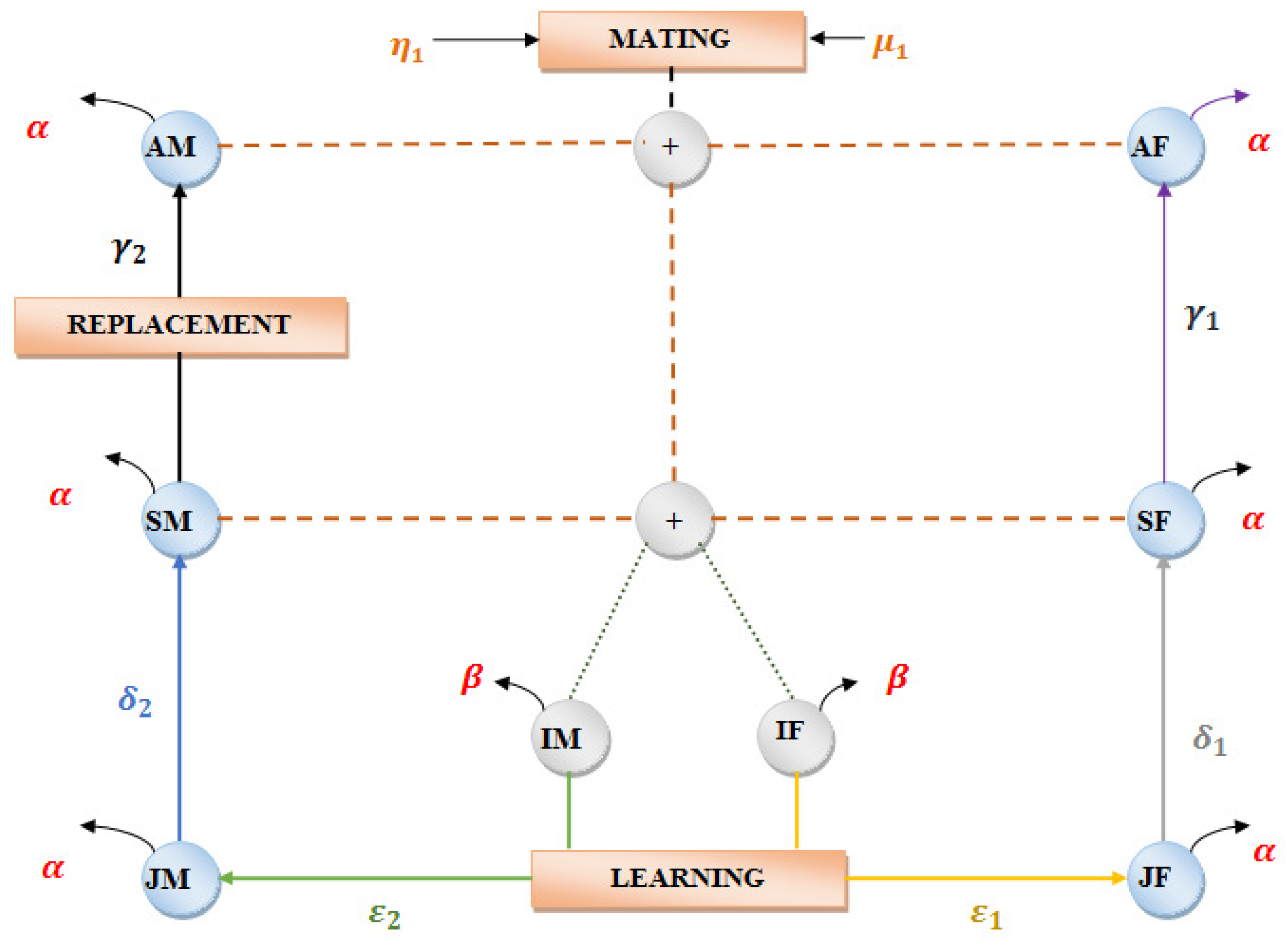
3.1. State Space Model for Java Macaque

Over the centuries, Java macaque monkeys have survived in this world because of their well-balanced behavior. This amply shows that the behavior of Java macaque monkeys has stability within the population. Then, the state space model for the Java macaque monkey in Figure 1 was designed using the demographic data shown in Table 1, obtained from the Ref. [57]. The demographic composition of the monkey population over the period of 1978 to 1982 was used to develop the state space model of the java monkey.
The generalized equation for female individuals in the state space models are represented as:
A F * = α A F + γ 1 S F
S F * = δ 1 J F γ 1 S F α S F
J F * = ε 1 I F δ 1 J F α J F
I F * = η 1 A M + μ 1 A F ε 1 I F β I F
η 1 = 2 3 μ 1 ,
where β , α are the death rate of the Infant (Offspring) and Non-Infant. Input variables u ( t ) are A F , S F , J F , I F , and the output variables y ( t ) are A F * , S F * , J F * , I F * with respect to the state variable α 1 , β 1 , γ 1 , δ 1 , ε 1 , μ 1 , η 1 . Additionally, AF, SF, JF and IF indicates the adult, sub-adult, juvenile and infant females.
Similarly, the generalized equation for male individuals in the population are presented as:
A M * = α A M + γ 2 S M
S M * = δ 2 J M γ 2 S M α S M
J M * = ε 2 I M δ 2 J M α J M
I M * = η 2 A M + μ 2 A F ε 2 I M β I M
η 2 = 2 3 μ 2 ,
where β , α are the death rate of the Infant (Offspring) and Non-Infant. Input variables u ( t ) are A M , S M , J M , I M and the output variable y ( t ) are A M * , S M * , J M * , I M * with respect to state variable α 2 , β 2 , γ 2 , δ 2 , ε 2 , μ 2 , η 2 . Additionally, AM, SM, JM and IM indicate the adult, sub-adult, or stray, juvenile, and infant males.
By using the state space model, we generated the transition matrix, which helps in proving the stability of the population using the α - diagonally dominant method, which has been clearly explained in the supplementary documents.

4. Java Macaque Monkey Algorithm Modeling

The Java Macaque Algorithm (JMA) is a meta-heuristic algorithm based on the genetic and social behavior of the java monkey. Initially, it starts with a population of the random solution and explores the search space to find the optimal. The life cycle of the Java macaque consists of selecting, mating, male replacement, and learning. Hence, the intelligent behavior of the java monkey does well to solve large-scale optimization problems. Moreover, it also demonstrates the behavior of Java macaques, and exhibits their adaptive learning, genetic, and social behavior and how they often respond according to changes in their environment, which maintains the global order emerging from the interaction of the java monkey. Thus, the life cycle of the java monkey could be transformed as the algorithm model for solving the real-world optimization problem.

4.1. JMA—Preamble

In the primitive of the Java macaque monkey, the search agents are divided into two types, known as the ‘Male’ and ‘Female’ Java macaque. The nature of male and female search agents is to produce different cooperative behavior depending on its gender. Then, the Java macaque exhibits a multi-group population that is utilized to achieve the best performance.
The population of a Java macaque leaves in g-groups and N-individuals in the group.
P O P = { G i } i = 1 , 2 , , g = { M j } j = 1 , 2 , , M s i z e { F k } k = 1 , 2 , , F s i z e s . t ( G i M , F : M F ) ,
where G i presents the group i with M s i z e of male individuals and F s i z e of female individuals in the population. The initialization process starts with a minimum number of individuals in the group with respect to the problem size. Then the casual system is utilized to control the size of the population in every group. | G i | , with a population size which consists of a number of male individuals M s i z e and female individuals F s i z e , is defined as:
M s i z e = f l o o r [ 0.9 r a n d ( 0.25 , 0.4 ) * | G i | ]
F s i z e = f l o o r [ 0.9 r a n d ( 0.45 , 0.6 ) * | G i | ]
M s i z e + F s i z e A c t s i z e : A c t s i z e R * .

4.2. JMA—Fitness Evaluation

The Java macaque depends on the genetic and social behavior in which dominant individuals are likely to be a winner in a problem space. The fitness evaluation indicates how far the individual is converged concerning the problem space. Fitness evaluation predicts the probability and survival rate of the individual to be transferred to the next generation of the population and is defined as:
minimize F ( Ψ ) s . t Ψ G ,
where ψ denotes an individual of x-dimensional integer vector ψ i = ( ψ 1 , ψ 2 , , ψ x ) , G represent the feasible region of the search space, and F R , where F is the optimization value.

4.3. JMA—Categorization

The basic structure of the java monkey follows the dominant hierarchy where the higher-ranking individuals dominate the remaining lower-ranking individuals in the group. The dominant male of the group also shows its dominance in accessing food, places, and other resources. Likewise, the dominant female of the group receives more access to resources and protection from a dominant male. Thus, the dominance hierarchy is based on evaluations of fitness value. Hence, the individuals are subdivided into higher-ranking or non-dominated (dominant) individuals and lower-ranking or dominated (non-dominant) individuals. Therefore, the individual ranking is based on the fitness value.The best individual in the group is known as the “Alpha” individual. Then, the `Alpha Male’ is the best male, and the `Alpha Female’ is the best female individual in the group. These are represented as follows:
A M i = m i n { F ( Ψ j | j { M } i , i { G i } }
A F i = m i n { F ( Ψ j | j { F } i , i { G i } } ,
where A M i and A F i are the local optimal solution for the problem X from the group { G i } . Therefore, the A M i , A F i X , and it is better than other individuals from the set { M } i and { F } i , where ( A M i , A F i G ( A M , A F X : F ( A M i ) < { M } i , F ( A F i ) < { F } i ) ) .
The global best individual from the set { A M } and { A F } are selected using:
[ G M , G F ] = min { { A M } , { A F } } ,
where G M , G F X are globally the best solution for the individual from the P O P .
Then the set of dominant and non-dominant (subordinate) male and female individuals in the group can also be formulated using the fitness value.
Ψ , Ψ * { M } then = Ψ { D S } , i f F ( Ψ ) > F ( Ψ * ) Ψ * { D S } , Ψ { N D S } , o t h e r w i s e ,
Ψ , Ψ * { F } then = Ψ { N D S } F , i f F ( Ψ ) > F ( Ψ * ) Ψ * { N D S } F , Ψ { D S } F , o t h e r w i s e ,
where both Ψ and Ψ * are either distinct male or female individuals from the G i . The non-dominant set of male and female individuals are represented as { N D S } M and { N D S } F . Similarly, the dominant male and female individuals are presented as { D S } M and  { D S } F .

4.4. JMA—Mating

Mating is an important operator in the Java macaque algorithm that ensures group survival and also enables the exchange of genetic information and social behavior between individuals. In particular, the dominant males have the privilege of mating with dominant females. Hence, non-dominant males may also have a lesser chance of mating due to the special prerequisite of dominance. The selection of individuals in the mating process plays an important role in generating populations for the next generation. Specifically, if the selection process depends only on a dominant individual, this may lead to local optima and reduce population diversity. Thus, the non-dominant individuals are also selected to perform mating operations with the probability ratio, which maintains diversity among individuals. Mating is the search process which is used to exploit the problem space X . Mating between males Ψ m and females Ψ f is either from the set {NDS} or {DS}. Then, new offspring Ψ o f f are generated as follows:
Ψ o f f = M a t i n g ( Ψ m , Ψ f ) s . t Ψ m , Ψ f G i ,
where the uniform crossover is used for the discrete optimization problem, and the simulated binary crossover for the continuous optimization problem.
The age of the Infant Male (IM) and Infant Female (IF) is set at 0, who then undergo a learning process to improve their fitness. The offspring generated in each { G i } from the mating process reaches sexual maturity S . Then the SM, SF and AF represent the Stray Male (subadult male), Subadult Female, and Adult Female, defined as the following:
Ψ I M = Ψ I M { J M } , i f A g e = 1 Ψ I M { I M } , o t h e r w i s e .
Ψ J M = Ψ J M { S M } , i f A g e = 4 Ψ J M { J M } , o t h e r w i s e .
Ψ I F = Ψ I F { J F } , i f A g e = 1 Ψ I F { I F } , o t h e r w i s e .
Ψ J F = Ψ J F { S F } , i f A g e = 3 Ψ J F { J F } , o t h e r w i s e ;
Ψ S F = Ψ S F { A F } , i f A g e = 5 Ψ S F { S F } , o t h e r w i s e ,
where A g e indicates the age of the individual. Similarly, if the Age = 5, then the Juvenile Female (JF) is moved to the set of Adult Females (AFs).

4.5. JMA—Male Replacement

The new offspring generated from the mating operation undergo a learning process from the dominant individual and the circumstances of the environment. Male replacement plays an important role in the Java macaque algorithm where the stray male chooses another group to reside in and replace the existing dominant male in the group. This is also considered as swarm behavior, where the stray male has to find a suitable position in the ruling hierarchy of the male. On the contrary, if a stray male cannot find a suitable position, then it is subjected to the risk of death. According to the fitness of the stray male, the replacement strategy variation plays out in a different manner. The male replacement can be defined as:
M R = R E P L A C E ( Ψ s m , Ψ m ) , i f F ( Ψ s m ) > F ( Ψ m ) Ψ s m { E S } , o t h e r w i s e ;
Ψ s m G i | | Ψ m { D S } M : ( Ψ m { G j } j = 1 , 2 , , M ) | i j ,
where R E P L A C E ( Ψ s m , Ψ m ) is the replacement process with the stray Ψ s m and dominant Ψ m male. Then { E S } is the elimination set where the individuals are eliminated from the population.

4.6. JMA—Learning

In this stage, the individuals in the population set can improve their fitness to reach the dominant individual set. The efficiency of the individual is improved based on the environment and social behavior. However, the potential of this learning process is to increase efficiency when compared with the current dominant hierarchy. Exploration is achieved by the learning method which enhances the fitness of an individual and also attains the optimal solution. The learning method is applied to the Java macaque algorithm to attain the desired results in global optimum, and this can be represented as follows:
L e a r n i n g = { P o P , G , δ , L ( Ψ ) , F ( Ψ ) , X } ,
where P O P represents the set of the individual, G is the feasible search space of the solution, F ( Ψ ) is the fitness function, X is the problem space of the optimization problem, and δ is referred to as the learning rate of the individual which is uniformly distributed ( 0 δ 1 ) . Then, the learning process is L ( Ψ k , i , j ) : Ψ G | x X .

5. Continuous Optimization Problem

In the continuous optimization problem, each decision variable may take any value between the range of constraints. Thus, the search space of continuous optimization may exponentially increase with the associated constraints. The initial difference between the continuous and discrete optimization is the representation of the individual with regard to a continuous search space.The java macaque for the continuous optimization algorithm consists of significant features selection, categorization, mating, male replacement and learning behavior. The Algorithm 1 clearly describes the computational methodology of java macaque optimization algorithm.
Definition 1.
The individuals are mapped ( m a p : G X ) between the dimension vector of the search space G to a dimensional vector in the problem space X . In the continuous optimization problem, the individuals are mapped to the number of decision variables ( N O D ) and represented as the dimension vector of the problem space.
Ψ = { ψ 1 , ψ 2 , , ψ N O D } Ψ . ψ G i , i 1 , 2 , , N O D ,
Ψ . x X : m a p ( Ψ . ψ ) = Ψ . x
where Ψ is a vector of decision variable { ψ 1 , ψ 2 , , ψ N O D } in the search space G . Each individual for the continuous function is represented as Ψ R and G = X R . Then the next level of difference in the continuous optimization problem is the evaluation of the fitness value of the individual.
Definition 2.
The generic form of the fitness evaluation is presented as follows:
M i n i m i z e F ( Ψ )
S . t Ψ X ,
where F ( Ψ ) is the fitness value of individuals with respect to the continuous optimization problem, and X is the decision space { F : X R N O C : l b i Ψ i u b i } with the upper bound ( u b ) and the lower bound ( l b ) of individual Ψ .
Then the remaining processes, like selecting the alpha male, alpha female, global best individual, and subdividing the population into dominated and non-dominated individuals, are completed using the fitness value.
Definition 3.
Mating is an important search process of JMA which is used to exploit the continuous search space G . Thus, the mating process is redefined with respect to the continuous search space. Mating between males Ψ m and females Ψ f is either from the set {DS} or {NDS}. Therefore, A i and I i are obtained from m a x ( ψ i m , ψ i f ) and m i n ( ψ i m , ψ i f ) . Then, new offspring Ψ o f f are generated as follows [58,59,60]:
Ψ o f f = M a t i n g ( Ψ m , Ψ f ) s . t Ψ m , Ψ f G i
| o f f | = { P ( A ) * ( | G i | A c t s i z e }
Ψ o f f 0 = 0.5 [ ( A i + I i ) θ 0 × ( A i I i ) ]
Ψ o f f 1 = 0.5 [ ( A i + I i ) + θ 1 × ( A i I i ) ] ,
where Ψ o f f 0 and Ψ o f f 1 are two new offspring generated from the crossover, and θ j ( j = 0 , 1 ) can be incurred as
θ j = ( C j × D j ) 1 ζ + 1 , i f C j 1 / D j ( 1 2 C j × D j ) 1 ζ + 1 , o t h e r w i s e ,
where C j is a uniformly distributed random number between [0,1] and θ is the distributed crossover index of offspring related to the parent’s natal code. Then D j ( j = 0 , 1 ) is generated by the assumption A i I i :
D j = 2 ( A i I i A i + I i 2 l b i ) ( ζ + 1 ) j = 0 2 ( A i I i 2 u b i A i I i ) ( ζ + 1 ) j = 1 ,
where l b i and u b i indicate the upper and lower bound of the decision variable.
Definition 4.
The learning process is adopted to improve the fitness value of the individual with respect to the problem space. Then, the learning process of the Java macaque may change with respect to the environment. Then the learning model for the continuous optimization problem is defined as follows:
L e a r n i n g = { P o P , G , δ , L ( Ψ k ) , F ( Ψ ) , X }
where P O P represents the set of individuals, G is the feasible search space of solutions, F ( Ψ ) is the fitness function, and δ indicates the learning rate of the individual in linear decreasing order ( 0 δ 1 ) . Then, the learning process of the individual is given by
L 1 ( Ψ G M , Ψ k ) : = Ψ G M ( 2 · δ · r 1 δ ) | 2 · r 2 · Ψ G M Ψ k | ,
where r 1 , r 2 are the random vectors between [0,1]. Similarly, the learning process of the individual Ψ k is performed between the global best female L 2 ( Ψ G F , Ψ k ) , alpha male L 3 ( Ψ A M , Ψ k ) and alpha female L 4 ( Ψ A F , Ψ k ) . Then, the individual Ψ k is modified as follows:
Ψ k = L 1 + L 2 + L 3 + L 4 4 ,
where Ψ i is the individual obtained from the learning process and replaced in the POP.
Algorithm 1 JMAC: Java Macaque Algorithm for Continuous Optimization Problem.
  • Input: N number of individuals, g number of groups, F is the fitness function.
  • Output: G B A M , G B F M , P O P
  • Step 1: [Initialization] The initial Population is initialized using a random seeding technique using Equation (29).
  • Step 2: [Evaluation] Each individual in the population is evaluated using the fitness function, as represented in Equation (30).
  • Step 3: The various categories of search agents are classified as:
  •     (a) [Alpha Individual] Determine the AlphaMale and AlphaFemale in each group using Equations (16) and (17).
  •     (b) [GB-Alpha Individual] Select the best individual from the AlphaMale and AlphaFemale sets using Equation (18).
  •     (c) [NDS and DS] Male and Female individual sets are further divided into dominant and non-dominant solutions using Equations (19) and (20).
  • Step 4: [Mating] Then the new offsprings are generated using the mating process, defined as in Equation (31).
  • Step 5: [Evaluation of Offspring] The fitness values of offspring are evaluated and the stray male and female are determined.
  • Step 6: [Male Replacement] The stray male finds a suitable group to replace the dominant male.
  • Step 7: [Learning] The fitness value of the individual is improved by moving the global best and alpha individuals by Equation (36).
  • Step 8: [Termination] The population is maintained by using Equation (11) and the above process is repeated from Step 2 until termination criteria are satisfied.

5.1. Experimentation and Result Analysis of Continuous Optimization Problem

In this section of experimentation, the benchmark function is taken from the popular literature [61,62] and used for analyzing the performance of the Java macaque algorithm. The performance of the proposed Java macaque algorithm is measured on 23 benchmark functions. The benchmark function utilized for the experimentation process consists of the 7 unimodal functions, 6 multimodal functions, and 10 fixed-dimension multimodal functions, where the dimension of the function is indicated in Dim, the upper and lower bound of the search space is referred to using Range, and finally, the optimal value of the benchmark function is indicated using the f m i n .
In the experimentation process, the proposed JMA is compared with the dominant algorithm from the literature, such as the grey wolf optimization (GWO) technique [61] and spider monkey algorithm (SMO) [12]. For all the algorithms, the population size was fixed as 200, stopping criteria were set as 100 iterations, and the primary population was produced using the random population seeding techniques. Every algorithm executed the 30 independent runs for each benchmark function, and the evaluation of the algorithm was measured using statistical measures such as the mean and standard deviation, as referred to in the literature [61,62]. Further, the best result is mentioned in bold font for reference in the respective table.

5.1.1. Result Analysis for Unimodal Benchmark Functions

The unimodal benchmark functions are suitable for analyzing the exploitation capability of the algorithm because it contains only one global optimum. Table 2 clearly shows a list of unimodal benchmark functions which is used for the experimentation process, and the function has different properties, like convex and non-convex shaped, non-differentiable, discontinuous, scalable, separable, and non-separable properties. Table 3 clearly shows the results of SMO, GWO and JMA on the unimodal benchmark functions. The performance of the proposed Java macaque optimization algorithm has clear dominance over the other two algorithms. In particular, the JMA attains the best results in both means and standard deviation on all the unimodel instances. GWO typically performs well in F5 and F6 in terms of means value, but struggles to outperform JMA. The Figure 2 facilitates the clear illustration that JMA dominates the other algorithm in terms of better convergence. The JMA has a dominant exploitation capability and can achieve a well-converged population. Further, it can clearly be depicted via standard deviations.

5.1.2. Multimodal Benchmark Function

The next important set of test functions used for the experimentation process is multimodal benchmark functions. The multimodal functions are utilized for analyzing the exploration potential of the algorithm because of its multiple local minima. Further, the benchmark function measures the global exploration capability of the algorithm, and an increase in dimension exponentially increases the number of local optima in the search space. Table 4 shows the list of multimodal benchmark functions for the experimentation.
The result illustrated in Table 5 and Figure 3 exhibits the performance of existing and proposed algorithms in terms of means and standard deviation. From the table observation, it is clearly shown that the performance of JMA rules out the other two algorithms. The JMA demonstrates its significance in mean value as 0.00E+00, 8.88E-16, 0.00E+00, 3.87E-05 and 3.21E-04 for the instance of F9 to F13, whereas the GWO achieves only 8.74E+00, 7.69E-05, 1.45E-07, 6.52E-03 and 4.83E-04. Similarly, the performance of standard deviation also demonstrates the dominance of the proposed algorithm over the GWO and SMO. Hence, this observation clearly provides the proof that the exploring capability of the proposed algorithm is superior to the existing algorithms.

5.1.3. Fixed-Dimension Multimodal Benchmark Function

The final experimentation for a continuous Java macaque algorithm is experimented with using the fixed-dimension multimodal benchmark functions. In this test function, the dimension of the benchmark function is fixed, which is used to analyze the performance of the algorithm in terms of exploration, exploitation, and also to avoid the local minima. The list of benchmark functions used for experimentation is shown in Table 6.
The results described in Table 7 clearly show that the JMA attains better values for the performance measures by comparing the GWO and SMO. The mean values of JMA and GWO are same as 1 for the instance F14, but the JMA shows its dominance in the SD value as 0.194221, whereas the GWO reaches only 1.737368. Similarly, Table 7 portrays how the performance of the three algorithms are almost the same as for the instance F18, but the proposed algorithm dominates in standard deviation. On the other hand, the performance of JMA lacks in terms of standard deviation for the instances F20 and F22 by GWO, and F17 and F21 by SMO. However, the JMA algorithm outperformed the GWO and SMO in terms of mean value for instances like f14, F16, F18, F19, F20, F21, F22 and F23. The fixed-dimension multi-modal benchmark function is utilized for analysis in the performance of the algorithm due to its multiple local minima, exploitation, and exploration capabilities.
The result shown in Table 8 and sample Figure 4 helps to analyze the experimentation in terms of convergence. The means value of 30 independent runs for the best convergence value in iterations 1, 10, and 25 illustrates the search ability of algorithms. The best value obtained from the iteration limit of 1 clearly demonstrated stronger convergence behavior of the JMA over the GWO and SMO in terms of all the unimodal instances. Further, the JMA was able to attain a near-optimal value in just 25 iterations for instances like F1, F2, F3, F4 and F7 with respective values 8.56E-04, 1.09E-02, 2.76E-01, 1.16E-01,and 7.76E-04, respectively. Additionally, in the case of the multimodal benchmark function, the proposed JMA led to the existing algorithm by all means. Correspondingly, in terms of the fixed dimensional multimodal function, the proposed JMA outperforms the existing algorithm in almost all instances, except F17, F21, and F22. The SMO algorithm shows better performance in terms of F17 and F21, whereas the GWO dominates only in F22. This observation shows that the potential behavior of the proposed JMA prevails over the existing algorithm in terms of avoiding local optima and achieving exploitation, exploration, and strong convergence in minimum iteration.

6. Discrete Optimization Problem

The problem space of a discrete optimization problem is represented as the set of all feasible solutions that satisfy the constraint and the fitness function, which maps each element to the problem space. Thus, the discrete or combinatorial optimization problem searches for the optimal solution from the set of feasible solutions.
The generic form of the discrete optimization problem is represented as follows [63]:
M i n i m i z e F ( Ψ )
s u b j e c t t o Ψ G ,
where F : G Z is the objective function with discrete problem space, which maps each individual in the search space G to the problem space X and the set of feasible solutions is G X .
The individuals were generated with the mapping ( m a p : G X ) between the dimensional vector of the search space G to the dimensional vector in the problem space X . In the discrete optimization problem, the total number of elements ( N O C ) is represented as the dimensional vector of the problem space, and it must be mapped as the element of search spaces of individual.
Ψ = { c 1 , c 2 , , c N O C } Ψ . c G , Ψ . x X : m a p ( Ψ . c ) = Ψ . x ,
where Ψ is an individual, represented as a tuple ( Ψ . c , Ψ . x ) of a dimensional vector Ψ . c in the search space G and the corresponding dimensional vector Ψ . x = Ψ . c in the problem space X . G i presents the group i with M s i z e of male individuals and F s i z e of female individuals in the population. The initialization process starts with a minimum number of individuals in the group with respect to the problem size.
The learning process is a mechanism which adapts the learning model for enhancing individual fitness. However, it increases individual fitness by exploiting the search space with respect to the problem space. The individual Ψ in the P O P should improve its fitness value F ( Ψ ) via learning and increase the probability of attaining a global optimum. Then, the learning for discrete optimization is defined as:
L e a r n i n g = { P o P , G , δ , L ( Ψ k , i , j ) , F ( Ψ ) , X } ,
where P O P represents the set of individuals, G is the feasible search space of solutions, F ( Ψ ) is the fitness function, and δ is referred to as the learning rate of the individual between ( 0 δ 1 ) .
Then, L ( Ψ k , i , j ) is the learning process L ( Ψ k , i , j ) : Ψ G , i , j Ψ .
[ i , j ] = s o r t [ c e i l ( x * r a n d ( δ , 2 ) ) ] ,
where the two values are randomly generated for i and j. Thus, the x is in linear decreasing order, generated between max to 3 ( m a x G ) .
( C a s e 1 ) : L 1 ( Ψ , [ i , j ] ) = L ( Ψ , [ j , i ] )
( C a s e 2 ) : L 2 ( Ψ , i , j ) = L ( Ψ , j : 1 : i )
( C a s e 3 ) : L 3 ( Ψ , i , j ) = L ( Ψ , [ i + 1 : j i ] )
( C a s e 4 ) : L 4 ( Ψ , i , j ) = L ( Ψ , i , j )
Ψ * = b e s t { F ( L 1 ) , F ( L 2 ) , F ( L 3 ) , F ( L 4 ) } where Ψ * P O P ,
where Ψ * is the best individual obtained from the different learning process and replaced Ψ k in the POP.

6.1. Experimentation and Result Analysis of Travelling Salesman Problem

The mathematical model for the travelling salesman problem is formulated as:
F = m i n i = 1 N O C 1 D ( C i , C i + 1 ) + D ( C N O C , C 1 ) ,
where D ( C i , C i + 1 ) is the distance between two cities C i and C i + 1 and D ( C N O C , C 1 ) indicate the tour between the last city C N O C and first city C 1 .
The standard experimental setup for the proposed Java macaque algorithm is as follows: (i) the initial population was randomly generated with 60 individuals in each group (m = 60); (ii) the number of groups (n = 5); (iii) executed up to 1000 iterations. The performance of the proposed JMA is correlated with an Imperialist Competitive Algorithm with a particle swarm optimization (ICA-PSO) [64], Fast Opposite Gradient Search with Ant Colony Optimization (FOGS-ACO) (Saenphon et al., 2014 [65]), and effective hybrid genetic algorithm (ECOGA) (Li and Zhang, 2007 [66]). Each algorithm was run on each instance 25 times, and hence, the best among the 25 runs was considered for analysis and validation purposes.

6.2. Parameter for Performance Assessment

This section briefly explains the list of parameters which evaluates the performance of the proposed Java macaque algorithm with the existing algorithm. It also helps to explore the efficiency of the proposed algorithm in various aspects. The various types of investigation parameters are the convergence rate, error rate, convergence diversity, and average convergence from the population. Thus, the parameter for the performance assessment is summarized as follows [3,67]:
Best Convergence Rate: In the experimentation, the best convergence rate measures the quality of the best individual obtained from the population in terms of percentage with regard to the optimal value. It can be measured as follows:
B e s t C o n v . ( % ) = 1 F ( Ψ b e s t ) O p t . F i t . O p t . F i t . × 100 ,
where F ( Ψ b e s t ) is the fitness of the best individual in the population and O p t . F i t . indicates the optimal fitness value of the instances.
Average Convergence Rate: The average percentage of the fitness value of the individual in the population with regard to the optimal fitness value is known as the average convergence rate. This can be calculated as:
A v g C o n v . ( % ) = 1 F ( P O P a v g ) O p t . F i t . O p t . F i t . × 100 ,
where F ( P O P a v g ) indicates the average fitness of all the individuals in the population.
Worst Convergence Rate: This parameter measures the percentage fitness of the worst individual in the population with regard to optimal fitness. It can be represented as:
W o r s t C o n v . ( % ) = 1 F ( Ψ w o r s t ) O p t . F i t . O p t . F i t . × 100 ,
where F ( Ψ w o r s t ) indicates the worst fitness value of the individual in the population.
Error rate: The error rate measures the percentage difference between the fitness value of the best individual and the optimal value of the instances. It can be given as:
E r r o r r a t e ( % ) = F ( Ψ b e s t ) O p t . F i t . O p t . F i t . × 100 .
Convergence diversity: Measures the difference between the convergence rate of the dominant individual and worst individuals found in the population. It can be represented as
C o n v . D i v ( % ) = B e s t C o n v . W o r s t C o n v .

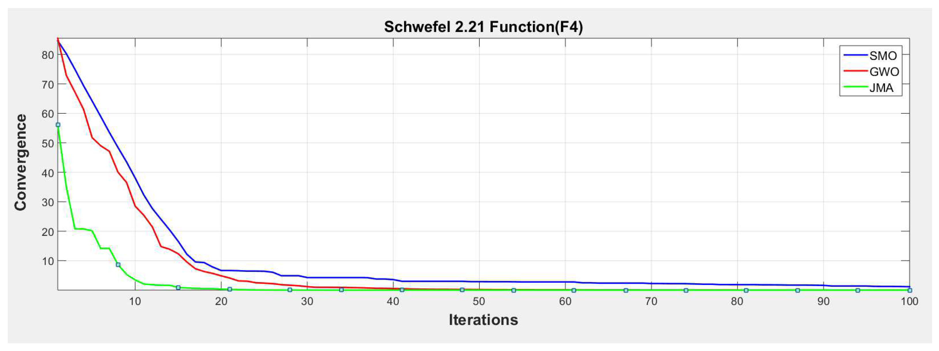
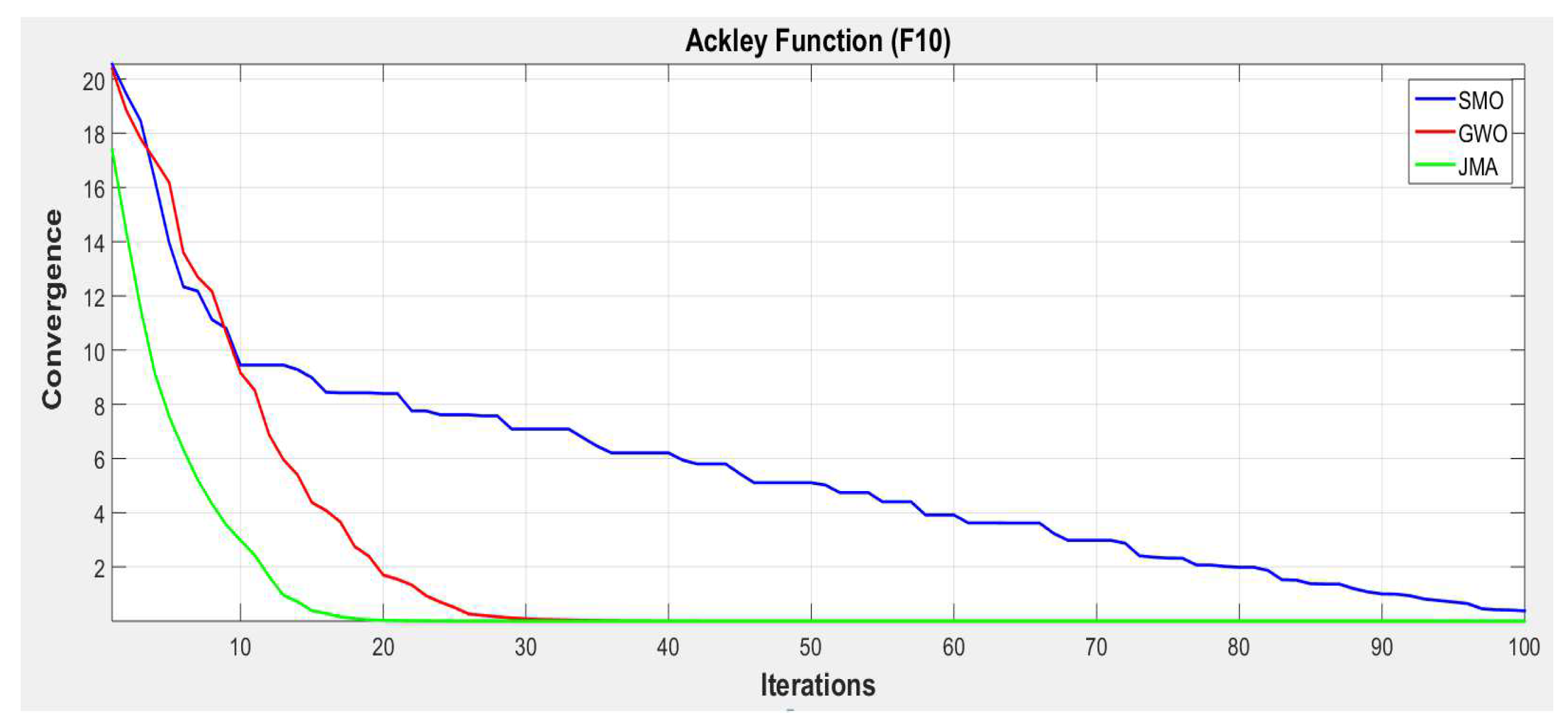
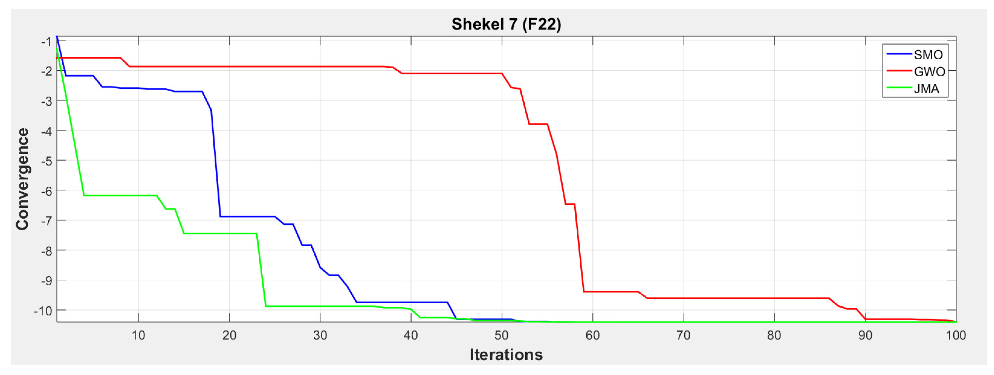
7. Result Analysis and Discussion

The computational results of the experimentation results are illustrated in this section. The Table 9 consists of the small-scale TSP instance, Table 10 has the results of the medium-scale TSP instance, and finally, Table 11 shows the results of large-scale instances. Thus, the experimentation were directed to evaluate the performance of the proposed JMA with other existing FOGS–ACO, ECO–GA and ICA–PSO. Consider, the sample instance eil51 for the result evaluation. The best convergence rate for ICA–PSO is 94.35%, FOGS–ACO is 92.88%, and ECO–GA is 97%, but the convergence rate of JMA is 100% for the instance eil76. Then the average convergence rate for ICA–PSO, FOGS–ACO, ECO–GA, and JMA are 65.64%, 80.39%, 70.94%, and 85.5%, respectively. On the other hand, this pattern of dominance is maintained in terms of error rate for all instances in Table 9. Further, the Table 11 depicts that the convergence rate of the proposed algorithm is above 99% for all the large-scale instances except rat575, whereas the existing ICA–PSO, FOGS–ACO, and ECO–GA are achieved above 90%, 93%, and 96% for the same. It can be observed from the Tables that the existing algorithm values for the average convergence rate is lower than the proposed JMA in most of the instances.The examination of the proposed algorithm dominated the existing ones in all the performance assessment parameters, except that the convergence diversity of ECO–GA is better than the proposed algorithm, but the proposed algorithm maintained well-balanced diversity in order to achieve optimal results.

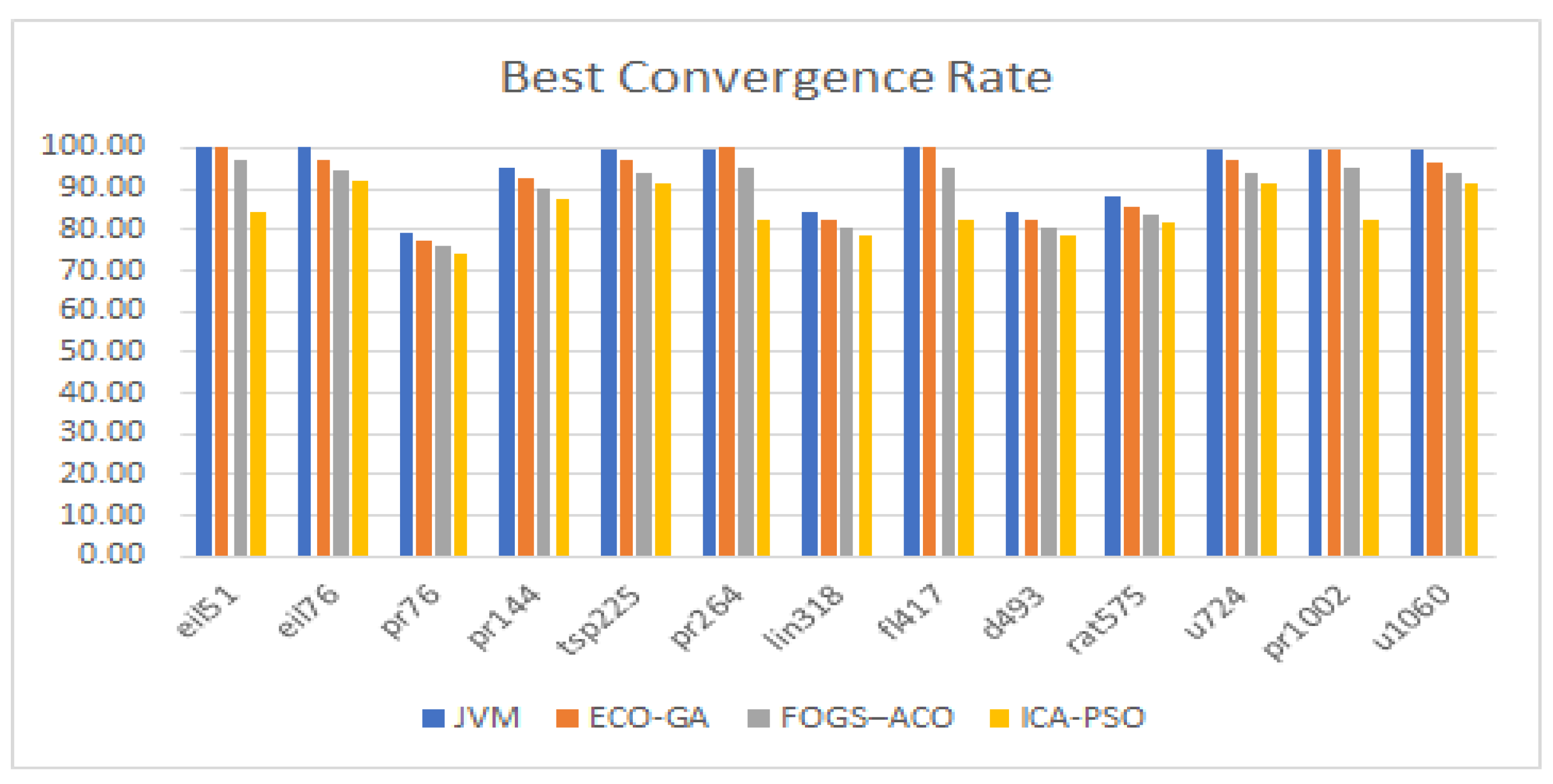
7.1. Analyzes Based on Best Convergence Rate

The best convergence rate reflects the effectiveness of the population-generated by optimization algorithm. Figure 5 depicts a comparison of the proposed algorithm to the existing algorithm in terms of convergence rate. The JMA holds lesser value as 74.23% for pr76 in small-scale instances. For medium-scale instances, the JMA holds 100% for the instance fl417. Then, the ECO–GA has the highest value of 99.97%, and JMA achieves convergence of 99.96% for the instance pr1002. As a result, on a medium scale, the instance lin318 has the lowest value of a 72.67% convergence rate in the ICA–PSO and the highest of 81.52 % for the JMA and 75.52 % for the FOGS–ACO, while the ECO–GA comes in second with a value of 78.44 %. In terms of convergence rate, the proposed Java macaque algorithm outperforms the existing algorithm.

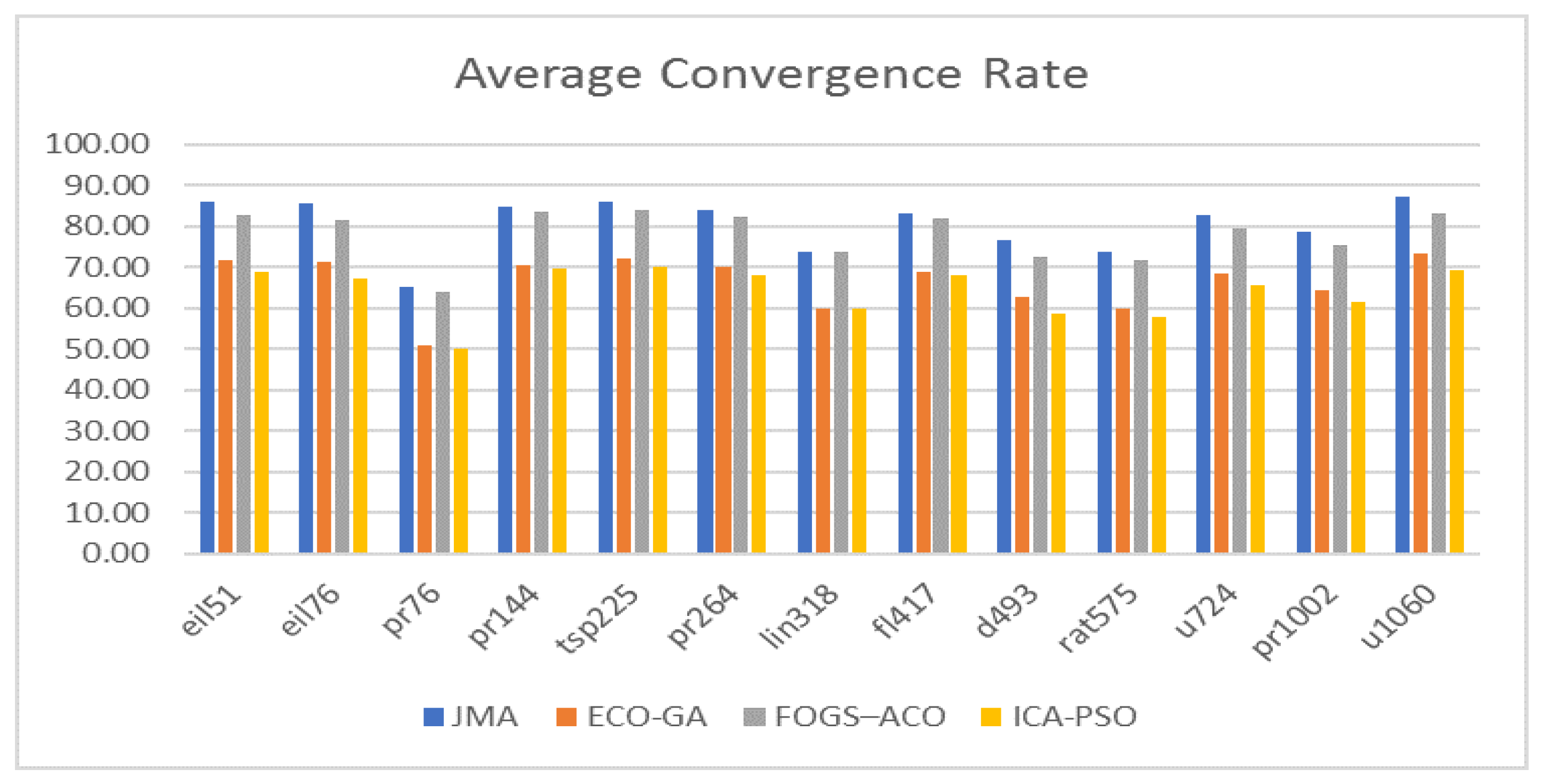
7.2. Analyzes Based on Average Convergence Rate

Figure 6 depicts the results of an average convergence rate comparison between the proposed algorithm and existing algorithms. As an outcome, the investigation in terms of average convergence for JMA revealed that it outperformed the other algorithm. The average convergence rate of JMA has to attain a value above 65%, but the FOGS–ACO, ECO–GA, and ICA–PSO obtained values above 64%, 51%, and 50%. The JMA achieved a maximum value of 87.36% for u1060, while the FOGS–ACO achieved 88.74% for pr144, and ECO–GA reached an average convergence of 73.34% for u1060, and lastly, the ICA–PSO attained a maximum of 70.02%, for instance, tsp225, respectively. While comparing the performance of JMA and FOGS–ACO for the average convergence rate, both algorithms perform quite well, but JMA dominates in many cases.

7.3. Analyzes Based on the Worst Convergence Rate

Figure 7 shows the performance of the experimentation with regard to the worst convergence rate. The proposed Java macaque algorithm dominated the existing algorithm by all means. For example, by acknowledging the occurrence of instance pr144, the ICA–PSO, FOGS–ACO, ECO–GA, and JMA obtained the worst convergence rates of 53.92%, 69.47%, 57.21%, and 72.62%, respectively. Then, by considering the pr1002 instance from a large-scale dataset, the proposed JMA and FOGS–ACO held an equal value of 55.14%, which was followed by an ECO–GA value of 41.13%, and the lowest value of 40.43% was attained by ICA–PSO. Further, in terms of medium–scale instances, the proposed Java macaque algorithm also shows its superiority over the existing algorithm, such as FOGS–ACO, ECO–GA, and ICA–PSO.

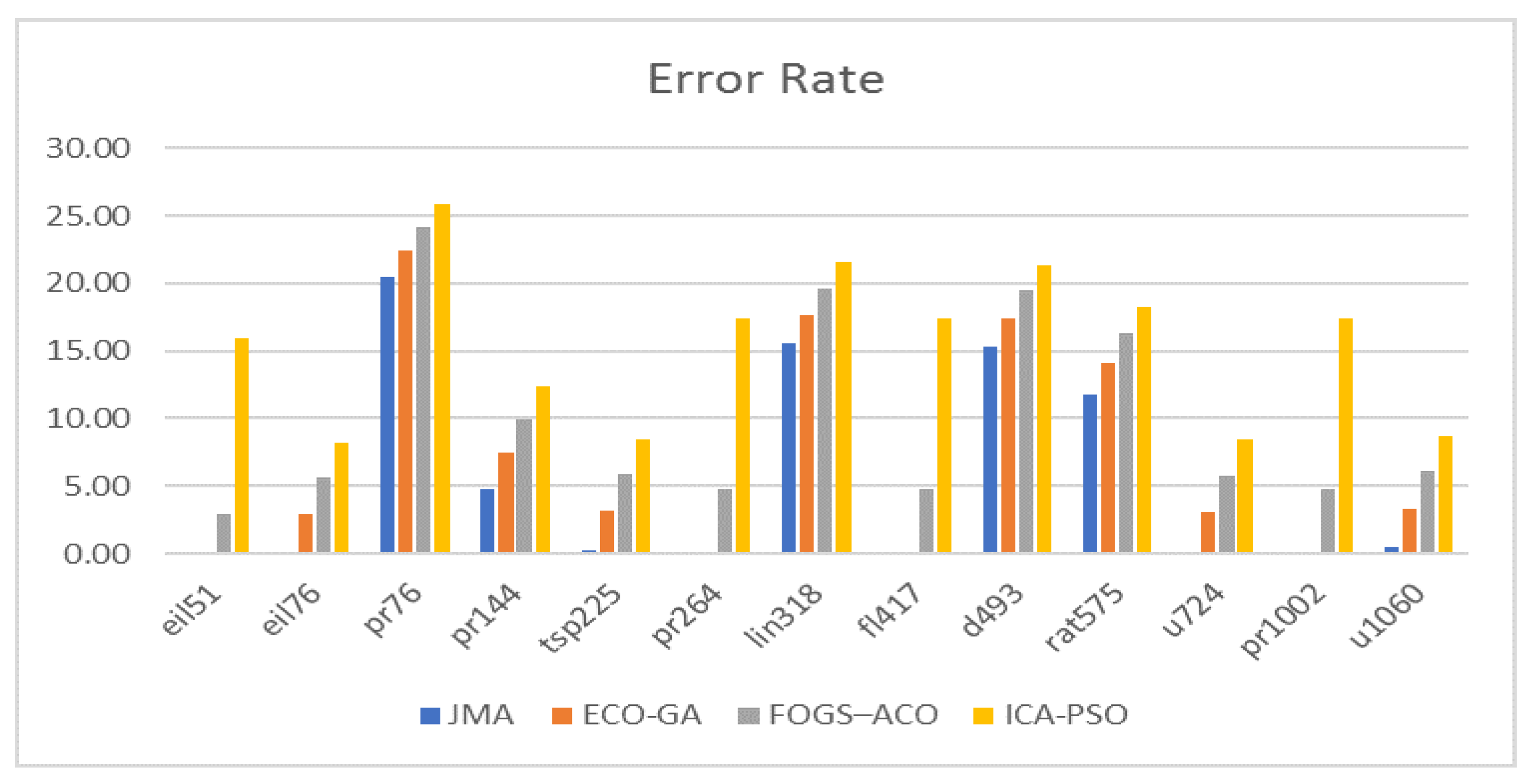
7.4. Analyzes Based on Error Rate

Figure 8 depicts the algorithm’s performance in terms of error rate. The best error rate shows how far the best individual’s convergence rate deviates from the optimal fitness value, whereas the worst error rate shows the difference between the worst individual’s convergence rate and the optimal solution.
Consequently, the maximum error rate of 25.83 percent for particle swarm optimization, 24.14 percent for ant colony optimization, 22.37 percent for genetic algorithm, Java macaque algorithm is 20.52 percent, and in that order. Meanwhile, the least error rate value for JMA was 0% for instances such as eil51, eil76, tsp225, pr264, fl417, u724, pr1002 and u1060, whereas the genetic algorithm had 0% for instances eil51, fl417 and the particle swarm optimization had an approximate value of 8% for instances eil76, tsp225 and u724, and FOGS–ACO has less than 3% for instance eil51, respectively. JMA obtained better performance compared with the existing algorithm.

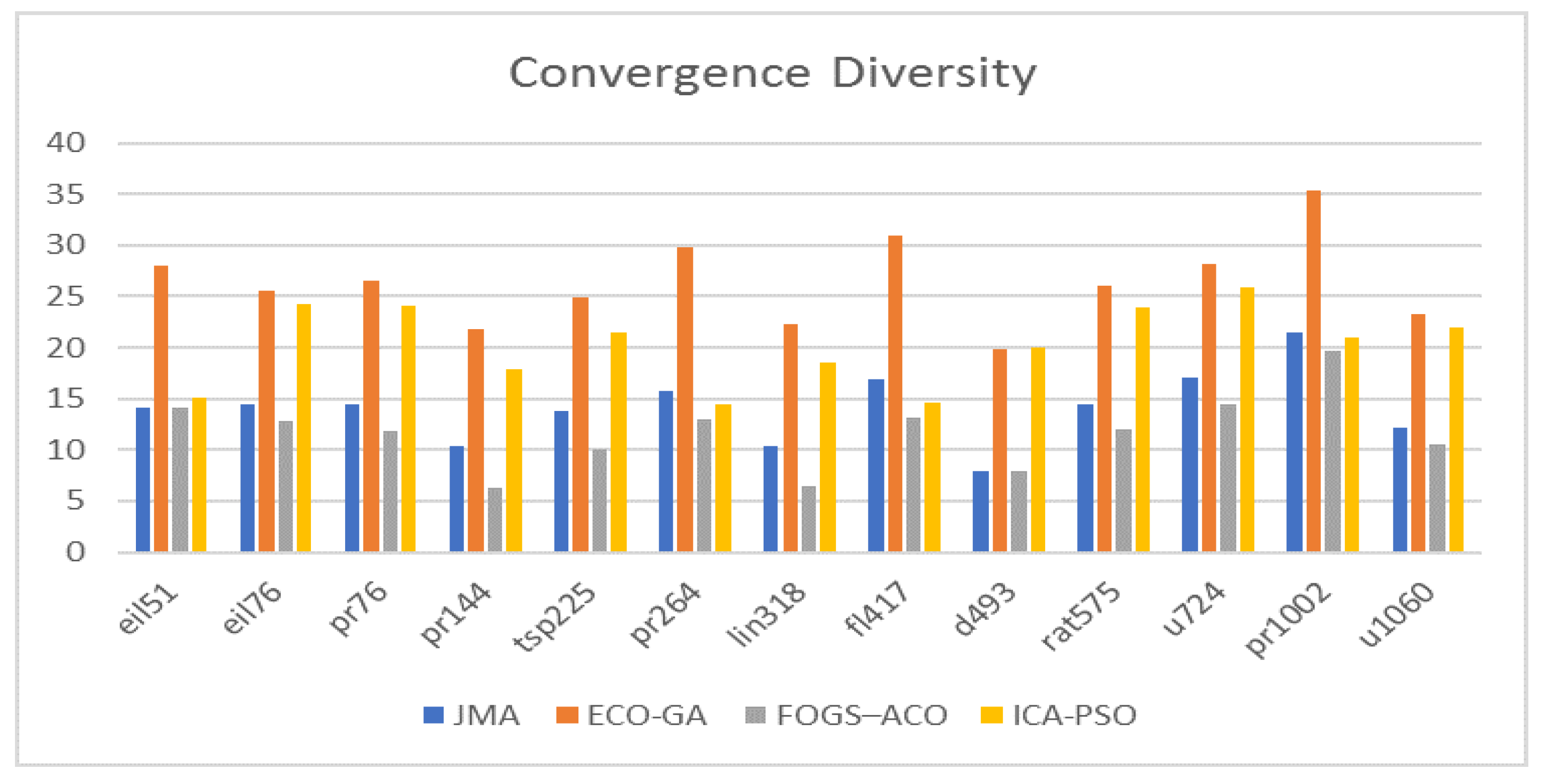
7.5. Analyzes Based on Convergence Diversity

One of the important assessment criteria that provides a concrete evidence of the optimal solution is convergence diversity. According to Figure 9, the performance of the existing ECO–GA surpassed the other algorithms in terms of diversity. For the sample instance u1060, the exisiting FOGS–ACO has a convergence diversity of 10.58%, the JMA has a convergence diversity for the instance as 12.19%, then the ICA–PSO has a value of 22%, whereas the ECO–GA achieved a highest value of 23.31%. The proposed JMA dominated the existing FOGS–ACO and was dominated by the other existing techniques, such as ECO–GA and ICA–PSO. Thus, the proposed JMA maintained the satisfactory level of convergence diversity among the population, and also achieved the best performance in terms of convergence with the existing algorithm.

8. Conclusions

The research proposed in this paper was motivated by the natural behavior of Java macaque monkeys and is suitable for solving real-world optimization problems. Thus, the Java macaque poses peculiar behavior with natural intelligence and a social hierarchy in an optimized way that well-suits the modeling of the novel Java macaque optimization algorithm. It was developed using the selection, categorisation, mating, male replacement, and learning behavior of the Java macaque. The important strategy exhibited by the population of the Java macaque is a dominance hierarchy, and that was incorporated with the JMA as a selection process. Hence, the individuals with higher social ranking dominated other individuals in the population and mostly gained preference in the mating process. Further, it helped the individuals with dominant status to gain a higher probability of generating new infants when considered with low-ranking individuals. Then, the algorithm also utilises the male replacement model, which increases the adaptive search capability of the JMA. Further, the JMA utilises the learning model that enhances the performance of the individual by increasing fitness, which proportionally upgrades social status. Hence, the JMA utilises the different search operations, which maintains well-balanced exploration and exploitation in finding the optimal solution. The performance of the proposed algorithm was analyzed with discrete and continuous optimization problems. The experimentation of continuous optimization was extensively conducted on 23 benchmark functions with unimodal, multimodal and fixed-dimension multimodal functions, and the proposed JMA depicts its dominant performance over the GWO and SMO. The outcomes of the experimentation were discussed as follows: (1) The unimodal functions are suitable for analyzing the exploitation capability of the algorithm because they contain only one global optimum. Thus, the result from Table 3 clearly depicts the dominance of JMA over other techniques. Hence, the JMA is well-suited for solving problems with exploitation behavior. (2) The multimodal functions are utilized for analyzing the exploration potential of the algorithm because of its multiple local minima, that is, the global exploration capability of the algorithm increases with an exponential increase in the number of local optima in the search space. Further, the performance of the experimentation illustrated from Table 5 also shows the dominance of the proposed system. (3) The final experimentation for the continuous Java macaque algorithm was experimented using the fixed-dimension multimodal benchmark functions. In this, the dimension of the benchmark function is fixed, which is used to analyze the performance of the algorithm in terms of exploration and exploitation. The results described in Table 7 clearly show that the JMA is well-suited to maintain the balance between exploration and exploitation. Further, the experimentation conducted over a discrete optimization problem by using the travelling salesman problem has to maintain balanced exploration and exploration with a quality selection process to achieve an optimal result. Thus, the results evidently show the performance of JMA over the existing dominant algorithm, such as FOGS–ACO, ECO–GA and ICA–PSO. Thus, the robustness of the JMA over the continuous and discrete search space clearly illustrates its potential over the optimization problem.

9. Future Enhancements

Future research will be focused on the development of the novel Java macaque algorithm with a hyper-optimization-based parameter-controlling casual system which efficiently explores and exploits the search space. Hence, the algorithm utilises social hierarchy-based selection, mating, male replacement, and a learning process as the operation of JMA. On the other hand, the grooming behavior of females and aggression behavior of males can also be incorporated with the JMA for enhancing the search process in the future. This algorithm enhancement may indeed improve the efficiency of the proposed algorithm for solving different kinds of real-world problems.

Author Contributions

Conceptualization, S.R.; methodology, A.D.; validation, R.S. and M.R.; formal analysis, D.K.; writing—original draft preparation, D.K.; writing—review and editing, M.R. and A.G.; supervision, S.S.A. and A.S.A.; funding acquisition, S.S.A. All authors have read and agreed to the published version of the manuscript.

Funding

This research was supported by Taif University, Research Supporting Project Number (TURSP-2020/215), Taif University, Taif, Saudi Arabia.

Institutional Review Board Statement

Not applicable.

Informed Consent Statement

Not applicable.

Data Availability Statement

Data available on request due to restrictions.

Conflicts of Interest

The authors declare no conflict of interest.

Abbreviations

The following abbreviations are used in this manuscript:
NIOAsNature-Inspired Optimization Algorithms
TSPTravelling Salesman Problem
EAEvolutionary Algorithm
SISwarm Intelligence
GAGenetic Algorithm
DEDifferential Evolution
ACOAnt Colony Optimization
ABCArtificial Bee Colony
PSOParticle Swarm Optimization
FAFirefly Algorithm
CSCuckoo Search
MAMonkey Algorithm
SMOSpider Monkey Algorithm
ASMOAgeist Spider Monkey Algorithm
GWOGrey Wolf Optimization
JMAJava macaque Algorithm
KHKrill Herd
BFABacterial foraging algorithm
AISrtificial Immune System
CACulture Algorithm
RAReptile Algorithm
ICA-PSOImperialist Competitive Algorithm with particle swarm optimization
FOGS-ACOFast Opposite Gradient Search with Ant Colony Optimization
ECOGASEffective hybrid genetic algorithm
AMAdult Male
SMSub-Adult Male
JMJuvenile Male
IMInfant Male
AFAdult Female
SFSub-Adult Female
JFJuvenile Female
IFInfant Female
α Death rate of Infant
β Death rate of Non-Infant
POPPopulation of Java macaque
{ G i }presents the Group i
M s i z e Male individuals in the population
F s i z e female individuals in the population
F( Ψ )Fitness evaluation individuals
GM, GFGlobal best male and female
{DS}Dominant set of individuals
{NDS}Non-Dominant set of individuals
δ Learning rate of the individual

References

  1. Uniyal, N.; Pant, S.; Kumar, A.; Pant, P. Nature-inspired metaheuristic algorithms for optimization. Meta-Heuristic Optim. Tech. Appl. Eng. 2022, 10, 1. [Google Scholar] [CrossRef]
  2. Alsalibi, B.; Mirjalili, S.; Abualigah, L.; Gandomi, A.H. A Comprehensive Survey on the Recent Variants and Applications of Membrane-Inspired Evolutionary Algorithms. Arch. Comput. Methods Eng. 2022, 1–17. [Google Scholar] [CrossRef]
  3. Dinesh, K.; Amudhavel, J.; Rajakumar, R.; Dhavachelvan, P.; Subramanian, R. A novel self-organisation model for improving the performance of permutation coded genetic algorithm. Int. J. Adv. Intell. Paradig. 2020, 17, 299–322. [Google Scholar] [CrossRef]
  4. Storn, R.; Price, K. Differential evolution—A simple and efficient heuristic for global optimization over continuous spaces. J. Glob. Optim. 1997, 11, 341–359. [Google Scholar] [CrossRef]
  5. Liu, C.; Wu, L.; Huang, X.; Xiao, W. Improved dynamic adaptive ant colony optimization algorithm to solve pipe routing design. Knowl.-Based Syst. 2022, 237, 107846. [Google Scholar] [CrossRef]
  6. Karaboga, D.; Basturk, B. A powerful and efficient algorithm for numerical function optimization: Artificial bee colony (ABC) algorithm. J. Glob. Optim. 2007, 39, 459–471. [Google Scholar] [CrossRef]
  7. Latchoumi, T.; Balamurugan, K.; Dinesh, K.; Ezhilarasi, T. Particle swarm optimization approach for waterjet cavitation peening. Measurement 2019, 141, 184–189. [Google Scholar] [CrossRef]
  8. Cao, L.; Ben, K.; Peng, H.; Zhang, X. Enhancing firefly algorithm with adaptive multi-group mechanism. Appl. Intell. 2022, 1–21. [Google Scholar] [CrossRef]
  9. Tang, C.; Song, S.; Ji, J.; Tang, Y.; Tang, Z.; Todo, Y. A cuckoo search algorithm with scale-free population topology. Expert Syst. Appl. 2022, 188, 116049. [Google Scholar] [CrossRef]
  10. Yılmaz, S.; Küçüksille, E.U. A new modification approach on bat algorithm for solving optimization problems. Appl. Soft Comput. 2015, 28, 259–275. [Google Scholar] [CrossRef]
  11. Ahmed, O.; Hu, M.; Ren, F. PEDTARA: Priority-Based Energy Efficient, Delay and Temperature Aware Routing Algorithm Using Multi-Objective Genetic Chaotic Spider Monkey Optimization for Critical Data Transmission in WBANs. Electronics 2022, 11, 68. [Google Scholar] [CrossRef]
  12. Tarawneh, H.; Alhadid, I.; Khwaldeh, S.; Afaneh, S. An Intelligent Cloud Service Composition Optimization Using Spider Monkey and Multistage Forward Search Algorithms. Symmetry 2022, 14, 82. [Google Scholar] [CrossRef]
  13. Abualigah, L.; Abd Elaziz, M.; Sumari, P.; Geem, Z.W.; Gandomi, A.H. Reptile Search Algorithm (RSA): A nature-inspired meta-heuristic optimizer. Expert Syst. Appl. 2022, 191, 116158. [Google Scholar] [CrossRef]
  14. Jain, S. Mammals: Whale, Gray Wolf, and Bat Optimization. In Nature-Inspired Optimization Algorithms with Java; Apress: Berkeley, CA, USA, 2022. [Google Scholar] [CrossRef]
  15. Yang, X.S. Mathematical Analysis of Nature-Inspired Algorithms. In Nature-Inspired Algorithms and Applied Optimization; Springer: Cham, Switzerland, 2018; Volume 744. [Google Scholar] [CrossRef]
  16. Karunanidy, D.; Ramalingam, R.; Dumka, A.; Singh, R.; Alsukayti, I.; Anand, D.; Hamam, H.; Ibrahim, M. An Intelligent Optimized Route-Discovery Model for IoT-Based VANETs. Processes 2021, 9, 2171. [Google Scholar] [CrossRef]
  17. Qin, S.; Pi, D.; Shao, Z.; Xu, Y. Hybrid collaborative multi-objective fruit fly optimization algorithm for scheduling workflow in cloud environment. Swarm Evol. Comput. 2022, 68, 101008. [Google Scholar] [CrossRef]
  18. Dos Anjos, J.C.S.; Gross, J.L.G.; Matteussi, K.J.; González, G.V.; Leithardt, V.R.Q.; Geyer, C.F.R. An Algorithm to Minimize Energy Consumption and Elapsed Time for IoT Workloads in a Hybrid Architecture. Sensors 2021, 21, 2914. [Google Scholar] [CrossRef]
  19. Dinesh, K.; Subramanian, R.; Dweib, I.; Nandhini, M.; Mohamed, M.Y.N.; Rajakumar, R. Bi-directional self-organization technique for enhancing the genetic algorithm. In Proceedings of the 6th International Conference on Information Technology: IoT and Smart City, Hong Kong, 29 December 2018–31 December 2019; pp. 251–255. [Google Scholar] [CrossRef]
  20. Jana, S.; Dey, A.; Maji, A.K.; Pal, R.K. Solving Sudoku Using Neighbourhood-Based Mutation Approach of Genetic Algorithm. In Advanced Computing and Systems for Security: Volume 13; Springer: Singapore, 2022; pp. 153–167. [Google Scholar] [CrossRef]
  21. Al-Sharhan, S.; Bimba, A. Adaptive multi-parent crossover GA for feature optimization in epileptic seizure identification. Appl. Soft Comput. 2019, 75, 575–587. [Google Scholar] [CrossRef]
  22. Manicassamy, J.; Karunanidhi, D.; Pothula, S.; Thirumal, V.; Ponnurangam, D.; Ramalingam, S. GPS: A constraint-based gene position procurement in chromosome for solving large-scale multiobjective multiple knapsack problems. Front. Comput. Sci. 2018, 12, 101–121. [Google Scholar] [CrossRef]
  23. Zhang, P.; Yao, H.; Li, M.; Liu, Y. Virtual network embedding based on modified genetic algorithm. Peer-to-Peer Netw. Appl. 2019, 12, 481–492. [Google Scholar] [CrossRef]
  24. Gholami, O.; Sotskov, Y.N.; Werner, F. A genetic algorithm for hybrid job-shop scheduling problems with minimizing the makespan or mean flow time. J. Adv. Manuf. Syst. 2018, 17, 461–486. [Google Scholar] [CrossRef]
  25. Karunanidy, D.; Amudhavel, J.; Datchinamurthy, T.S.; Ramalingam, S. A Novel Java macaque Algorithm For Travelling Salesman Problem. IIOAB J. 2017, 8, 252–261. [Google Scholar]
  26. Dinesh, K.; Rajakumar, R.; Subramanian, R. Self-organisation migration technique for enhancing the permutation coded genetic algorithm. Int. J. Appl. Manag. Sci. 2021, 13, 15–36. [Google Scholar] [CrossRef]
  27. Santos, J.; Ferreira, A.; Flintsch, G. An adaptive hybrid genetic algorithm for pavement management. Int. J. Pavement Eng. 2019, 20, 266–286. [Google Scholar] [CrossRef]
  28. Luan, J.; Yao, Z.; Zhao, F.; Song, X. A novel method to solve supplier selection problem: Hybrid algorithm of genetic algorithm and ant colony optimization. Math. Comput. Simul. 2019, 156, 294–309. [Google Scholar] [CrossRef]
  29. Bujok, P.; Tvrdík, J.; Poláková, R. Comparison of nature-inspired population-based algorithms on continuous optimisation problems. Swarm Evol. Comput. 2019, 50, 100490. [Google Scholar] [CrossRef]
  30. Ramos-Figueroa, O.; Quiroz-Castellanos, M.; Mezura-Montes, E.; Kharel, R. Variation operators for grouping genetic algorithms: A review. Swarm Evol. Comput. 2021, 60, 100796. [Google Scholar] [CrossRef]
  31. Opara, K.R.; Arabas, J. Differential Evolution: A survey of theoretical analyzes. Swarm Evol. Comput. 2019, 44, 546–558. [Google Scholar] [CrossRef]
  32. Wang, X.; Wang, Y.; Wong, K.C.; Li, X. A self-adaptive weighted differential evolution approach for large-scale feature selection. Knowl.-Based Syst. 2022, 235, 107633. [Google Scholar] [CrossRef]
  33. Müller, F.M.; Bonilha, I.S. Hyper-Heuristic Based on ACO and Local Search for Dynamic Optimization Problems. Algorithms 2022, 15, 9. [Google Scholar] [CrossRef]
  34. Mahmoodi, L.; Aliyari Shoorehdeli, M. Comments on “A Novel Fault Diagnostics and Prediction Scheme Using a Nonlinear Observer With Artificial Immune System as an Online Approximator”. IEEE Trans. Control. Syst. Technol. 2017, 25, 2243–2246. [Google Scholar] [CrossRef]
  35. Coulter, N.; Moncayo, H. Artificial Immune System Optimized Support Vector Machine for Satellite Fault Detection. In Proceedings of the AIAA SCITECH 2022 Forum, San Diego, CA, USA, 3–7 January 2022; p. 1713. [Google Scholar] [CrossRef]
  36. Passino, K.M. Biomimicry of bacterial foraging for distributed optimization and control. IEEE Control. Syst. 2002, 22, 52–67. [Google Scholar]
  37. Hernández-Ocaña, B.; Chávez-Bosquez, O.; Hernández-Torruco, J.; Canul-Reich, J.; Pozos-Parra, P. Bacterial Foraging Optimization Algorithm for menu planning. IEEE Access 2018, 6, 8619–8629. [Google Scholar] [CrossRef]
  38. Awad, H.; Hafez, A. Optimal operation of under-frequency load shedding relays by hybrid optimization of particle swarm and bacterial foraging algorithms. Alex. Eng. J. 2022, 61, 763–774. [Google Scholar] [CrossRef]
  39. Wang, G.G.; Gandomi, A.H.; Alavi, A.H.; Deb, S. A hybrid method based on krill herd and quantum-behaved particle swarm optimization. Neural Comput. Appl. 2016, 27, 989–1006. [Google Scholar] [CrossRef]
  40. Saravanan, D.; Janakiraman, S.; Harshavardhanan, P.; Kumar, S.A.; Sathian, D. Enhanced Binary Krill Herd Algorithm for Effective Data Propagation in VANET. In Secure Communication for 5G and IoT Networks; Springer: Cham, Switzerland, 2022; pp. 221–235. [Google Scholar] [CrossRef]
  41. Yang, X.S.; He, X. Firefly algorithm: Recent advances and applications. Int. J. Swarm Intell. 2013, 1, 36–50. [Google Scholar] [CrossRef] [Green Version]
  42. Cheng, Z.; Song, H.; Chang, T.; Wang, J. An improved mixed-coded hybrid firefly algorithm for the mixed-discrete SSCGR problem. Expert Syst. Appl. 2022, 188, 116050. [Google Scholar] [CrossRef]
  43. Mohanty, P.P.; Nayak, S.K. A Modified Cuckoo Search Algorithm for Data Clustering. Int. J. Appl. Metaheuristic Comput. (IJAMC) 2022, 13, 1–32. [Google Scholar] [CrossRef]
  44. Kumar, S.; Kumari, R. Modified position update in spider monkey optimization algorithm. Int. J. Emerg. Technol. Comput. Appl. Sci. (IJETCAS) 2014, 2, 198–204. [Google Scholar]
  45. Wu, G.; Mallipeddi, R.; Suganthan, P.N.; Wang, R.; Chen, H. Differential evolution with multi-population based ensemble of mutation strategies. Inf. Sci. 2016, 329, 329–345. [Google Scholar] [CrossRef]
  46. Ma, H.; Shen, S.; Yu, M.; Yang, Z.; Fei, M.; Zhou, H. Multi-population techniques in nature inspired optimization algorithms: A comprehensive survey. Swarm Evol. Comput. 2019, 44, 365–387. [Google Scholar] [CrossRef]
  47. Xu, Z.; Liu, X.; Zhang, K.; He, J. Cultural transmission based multi-objective evolution strategy for evolutionary multitasking. Inf. Sci. 2022, 582, 215–242. [Google Scholar] [CrossRef]
  48. Warwas, K.; Tengler, S. Multi-population Genetic Algorithm with the Actor Model Approach to Determine Optimal Braking Torques of the Articulated Vehicle. In Intelligent Computing; Springer: Cham, Switzerland, 2022; Volume 283, pp. 56–74. [Google Scholar] [CrossRef]
  49. Hesar, A.S.; Kamel, S.R.; Houshmand, M. A quantum multi-objective optimization algorithm based on harmony search method. Soft Comput. 2021, 25, 9427–9439. [Google Scholar] [CrossRef]
  50. Zhang, Y.; Li, J.; Li, L. A Reward Population-Based Differential Genetic Harmony Search Algorithm. Algorithms 2022, 15, 23. [Google Scholar] [CrossRef]
  51. Van den Bercken, J.; Cools, A. Information-statistical analysis of factors determining ongoing behaviour and social interaction in Java monkeys (Macaca fascicularis). Anim. Behav. 1980, 28, 189–200. [Google Scholar] [CrossRef]
  52. Veenema, H.C.; Spruijt, B.M.; Gispen, W.H.; Van Hooff, J. Aging, dominance history, and social behavior in Java-monkeys (Macaca fascicularis). Neurobiol. Aging 1997, 18, 509–515. [Google Scholar] [CrossRef]
  53. Dewsbury, D.A. Dominance rank, copulatory behavior, and differential reproduction. Q. Rev. Biol. 1982, 57, 135–159. [Google Scholar] [CrossRef] [PubMed]
  54. Engelhardt, A.; Pfeifer, J.B.; Heistermann, M.; Niemitz, C.; van Hooff, J.A.; Hodges, J.K. Assessment of female reproductive status by male longtailed macaques, Macaca fascicularis, under natural conditions. Anim. Behav. 2004, 67, 915–924. [Google Scholar] [CrossRef]
  55. Sprague, D.S. Age, dominance rank, natal status, and tenure among male macaques. Am. J. Phys. Anthropol. 1998, 105, 511–521. [Google Scholar] [CrossRef]
  56. Dasser, V. A social concept in Java monkeys. Anim. Behav. 1988, 36, 225–230. [Google Scholar] [CrossRef]
  57. Paul, A.; Thommen, D. Timing of birth, female reproductive success and infant sex ratio in semifree-ranging Barbary macaques (Macaca sylvanus). Folia Primatol. 1984, 42, 2–16. [Google Scholar] [CrossRef]
  58. Durillo, J.J.; Nebro, A.J. jMetal: A Java framework for multi-objective optimization. Adv. Eng. Softw. 2011, 42, 760–771. [Google Scholar] [CrossRef]
  59. Deb, K.; Beyer, H.G. Self-Adaptive Genetic Algorithms with Simulated Binary Crossover. Evol. Comput. 9, 197–221. [CrossRef]
  60. Lin, Q.; Chen, J.; Zhan, Z.H.; Chen, W.N.; Coello, C.A.C.; Yin, Y.; Lin, C.M.; Zhang, J. A hybrid evolutionary immune algorithm for multiobjective optimization problems. IEEE Trans. Evol. Comput. 2016, 20, 711–729. [Google Scholar] [CrossRef]
  61. Meidani, K.; Hemmasian, A.; Mirjalili, S.; Barati Farimani, A. Adaptive grey wolf optimizer. Neural Comput. Appl. 2022, 1–21. [Google Scholar] [CrossRef]
  62. Zhang, L.; Liu, L.; Yang, X.S.; Dai, Y. A novel hybrid firefly algorithm for global optimization. PLoS ONE 2016, 11, e0163230. [Google Scholar] [CrossRef] [PubMed] [Green Version]
  63. Di Gaspero, L.; Schaerf, A.; Cadoli, M.; Slany, W.; Falaschi, M. Local Search Techniques for Scheduling Problems: Algorithms and Software Tool. Ph.D. Thesis, Università degli Studi di Udine, Udine, Italy, 2003. [Google Scholar]
  64. Idoumghar, L.; Chérin, N.; Siarry, P.; Roche, R.; Miraoui, A. Hybrid ICA–PSO algorithm for continuous optimization. Appl. Math. Comput. 2013, 219, 11149–11170. [Google Scholar] [CrossRef]
  65. Saenphon, T.; Phimoltares, S.; Lursinsap, C. Combining new fast opposite gradient search with ant colony optimization for solving travelling salesman problem. Eng. Appl. Artif. Intell. 2014, 35, 324–334. [Google Scholar] [CrossRef]
  66. Li, L.; Zhang, Y. An improved genetic algorithm for the traveling salesman problem. In International Conference on Intelligent Computing; Springer: Berlin/Heidelberg, Germany, 2007; Volume 2, pp. 208–216. [Google Scholar] [CrossRef]
  67. Paul, P.V.; Moganarangan, N.; Kumar, S.S.; Raju, R.; Vengattaraman, T.; Dhavachelvan, P. Performance analyzes over population seeding techniques of the permutation-coded genetic algorithm: An empirical study based on traveling salesman problems. Appl. Soft Comput. 2015, 32, 383–402. [Google Scholar] [CrossRef]
Figure 1. State space model of the Java macaque monkey.
Mathematics 10 00688 g001
Figure 2. Convergence Curve for Schwefel 2.21 Function (F4).
Mathematics 10 00688 g002
Figure 3. Convergence curve for the Ackley function (F10).
Mathematics 10 00688 g003
Figure 4. Convergence curve for Shekel 7 Function (F22).
Mathematics 10 00688 g004
Figure 5. Best convergence rate.
Mathematics 10 00688 g005
Figure 6. Average convergence rate.
Mathematics 10 00688 g006
Figure 7. Worst convergence rate.
Mathematics 10 00688 g007
Figure 8. Error rate.
Mathematics 10 00688 g008
Figure 9. Convergence diversity.
Mathematics 10 00688 g009
Table 1. Demographic composition of the monkey population (1978–1982).
ClassAge Years19781979198019811982
Adult Male≥7192530(1)39(3)63(2)
Adult Female≥551(1)57(1)68(1)76(1)91(1)
Subadult Male4–6254548(1)5443
Subadult Female471291625
Juvenile Male1–35543(2)47(1)5475
Juvenile Female1–43950(2)71(2)82(1)82(2)
Infant Male<116(3)15(3)25(3)36(2)37(5)
Infant Unsexed<225(1)32(2)28(1)27(1)38(5)
Infant Female<300(2)0(1)00
Total 237279326384454
Infant Mortality 2 8.8912.967.024.5411.76
Noninfant Mortality 1 0.512.112.151.231.31
Table 2. Benchmark Function.
FunctionDimRange f min
f 1 x = i = 1 n x i 2 30[−100, 100]0
f 2 x = i = 1 n x i + i = 1 n x i 30[−10, 10]0
f 3 x = i = 1 n j = 1 i x j 2 30[−100, 100]0
f 4 x = m a x i m u m i x i , 1 i n 30[−100, 100]0
f 5 x = i = 1 n 100 x i + 1 x i 2 2 + x i 1 2 30[−30, 30]0
f 6 x = i = 1 n x i + 0.5 2 30[−100, 100]0
f 7 x = i = 1 n i x i 4 + U ( 0 , 1 ) 30[−1.28, 1.28]0
Table 3. Experimental results of unimodal benchmark function.
FunctionTechniqueOptimal ValueBestSD
F1SMO09.64E-021.09E+04
GWO1.21E-077.92E+03
JMA1.06E-301.47E+03
F2SMO08.96E-012.45E+10
GWO3.18E-059.84E+08
JMA2.50E-171.40E+02
F3SMO01.28E+021.83E+04
GWO3.28E-011.67E+04
JMA5.43E-245.21E+03
F4SMO01.15E+001.93E+01
GWO3.31E-021.75E+01
JMA4.75E-146.63E+00
F5SMO08.85E+012.67E+07
GWO2.58E+012.20E+07
JMA2.81E+011.80E+06
F6SMO01.21E-011.23E+04
GWO3.89E-047.57E+03
JMA3.98E-042.09E+03
F7SMO03.15E-011.78E+01
GWO1.76E-037.61E+00
JMA1.15E-036.35E-01
Table 4. Multimodal benchmark function.
FunctionDimRange f min
f 8 x = i = 1 n x i sin x i 30[−500, 500]−418.9829 × 5
f 9 x = i = 1 n x i 2 10 cos 2 π x i + 10 30[−5.12, 5.12]0
f 10 x = 20 exp 0.2 1 n i = 1 n x i 2 exp 1 n i = 1 n cos 2 π x i + 20 + e 30[−32, 32]0
f 11 x = 1 4000 i = 1 n x i 2 i = 1 n cos x i i + 1 30[−600, 600]0
f 12 x = π n 10 sin π y 1 + i = 1 n 1 y i 1 2 1 + 10 sin 2 ( π y i + 1 ) + ( y n 1 ) 2 + i = 1 n u ( x i , 10 , 100 , 4 )
y i = 1 + x i + 1 4 u x i , a , k , m = k ( x i a ) m x i > a 0 a < x i < a k ( x i a ) m x i < a 30[−50, 50]0
f 13 x = 0.1 sin 2 3 π x 1 + i = 1 n x i 1 2 1 + sin 2 3 π x i + 1 + x n 1 2 1 + sin 2 2 π x n + i = 1 n u x i , 5 , 100 , 4 30[−50, 50]0
Table 5. Experimental results of the multimodal benchmark function.
FunctionTechniqueOptimal ValueBestSD
F8SMO−12569.5−4706.472.60E+02
GWO−4374.351.18E+03
JMA−3384.651.26E+01
F9SMO07.81E+016.70E+01
GWO8.74E+009.46E+01
JMA0.00E+005.04E+01
F10SMO03.78E-013.77E+00
GWO7.69E-054.85E+00
JMA8.88E-162.94E+00
F11SMO02.78E+001.76E+02
GWO1.45E-076.94E+01
JMA0.00E+001.46E+01
F12SMO01.36E-035.15E+07
GWO6.52E-037.12E+07
JMA3.87E-052.61E+06
F13SMO05.45E-021.07E+08
GWO4.83E-049.37E+07
JMA3.21E-049.53E+06
Table 6. Fixed-dimension multimodal benchmark function.
FunctionDimRange f min
f 14 x = 1 500 + j = 1 25 1 j + i = 1 2 ( x i a i j ) 6 1 2[−65, 65]1
f 15 ( x ) = i = 1 11 a i x 1 ( b i 2 + b i x 2 ) b i 2 + b i x 3 + x 4 2 4[−5, 5]0.00030
f 16 x = 4 x 1 2 2.1 x 1 4 + 1 3 x 1 6 + x 1 x 2 4 x 2 2 + 4 x 2 4 2[−5, 5]−1.0316
f 17 x = x 2 5.1 4 π 2 x 1 2 + 5 π x 1 6 2 + 10 1 1 8 π c o s x 1 + 10 2[−5, 5]0.398
f 18 x = 1 + x 1 + x 2 + 1 2 19 14 x 1 + 3 x 1 2 14 x 2 + 6 x 1 x 2 + 3 x 2 2 2[−2, 2]3
× 30 + 2 x 1 3 x 2 2 × 18 32 x 1 + 12 x 1 2 + 48 x 2 36 x 1 x 2 + 27 x 2 2
f 19 x = i = 1 4 c i e x p j = 1 3 a i j x j p i j 2 3[1, 3]−3.86
f 20 ( x ) = i = 1 4 c i e x p j = 1 6 a i j x j p i j 2 6[0, 1]−3.32
f 21 x = i = 1 5 X a i X a i T + c i 1 4[0, 10]−10.1532
f 22 x = i = 1 7 X a i X a i T + c i 1 4[0, 10]−10.4028
f 23 x = i = 1 10 X a i X a i T + c i 1 4[0, 10]−10.5363
Table 7. Experimental results of the fixed-dimension multimodal benchmark function.
FunctionTechniqueOptimal ValueBestSD
F14SMO11.08E+001.13E+00
GWO1.00E+001.74E+00
JMA1.00E+001.94E-01
F15SMO0.00034.26E-044.18E-03
GWO3.08E-045.26E-04
JMA3.23E-049.30E-03
F16SMO−1.0316−1.03E+001.87E-02
GWO−1.03E+006.11E-02
JMA−1.03E+007.90E-03
F17SMO0.3983.98E-013.81E-02
GWO3.98E-017.42E-02
JMA3.98E-014.15E-02
F18SMO33.00E+008.54E-01
GWO3.00E+001.85E+00
JMA3.00E+006.43E-01
F19SMO−3.86−3.86E+003.67E-02
GWO−3.86E+003.11E-02
JMA−3.86E+002.45E-02
F20SMO−3.22−3.32E+001.28E-01
GWO−3.32E+005.63E-02
JMA−3.07E+001.43E-01
F21SMO−10.1532−1.02E+012.13E+00
GWO−1.01E+012.38E+00
JMA−1.02E+012.65E+00
F22SMO−10.4028−1.04E+013.40E+00
GWO−1.04E+012.42E+00
JMA−1.04E+013.03E+00
F23SMO−10.5363−1.05E+012.71E+00
GWO−1.05E+012.87E+00
JMA−1.05E+012.52E+00
Table 8. Best values obtained by JMA, GWO and SMO in Iterations 1, 10, and 25.
FunctionTechniqueIterationFunctionTechniqueIteration
1102511025
F1SMO5.66E+041.28E+042.29E+02F13SMO9.37E+083.10E+053.31E+01
GWO5.73E+042.23E+031.84E+00GWO8.34E+086.01E+042.27E+00
JMA1.11E+042.58E+018.56E-04JMA9.58E+077.49E+002.52E+00
F2SMO2.46E+116.32E+013.81E+01F14SMO1.04E+011.00E+009.98E-01
GWO9.89E+091.34E+013.73E-01GWO1.09E+012.07E+009.99E-01
JMA1.41E+032.11E+001.09E-02JMA2.10E+001.20E+009.98E-01
F3SMO1.01E+052.45E+042.97E+03F15SMO4.12E-024.70E-038.52E-04
GWO1.05E+052.27E+042.25E+03GWO3.47E-031.05E-037.26E-04
JMA3.93E+041.56E+032.76E-01JMA9.36E-027.02E-047.02E-04
F4SMO8.89E+014.00E+017.37E+00F16SMO−8.52E-01−1.03E+00−1.03E+00
GWO7.72E+013.25E+014.02E+00GWO−4.18E-01−1.03E+00−1.03E+00
JMA4.18E+015.90E+001.16E-01JMA−9.76E-01−1.03E+00−1.03E+00
F5SMO2.51E+088.24E+057.85E+04F17SMO7.74E-014.00E-013.98E-01
GWO1.90E+084.18E+051.34E+02GWO6.84E-015.56E-013.99E-01
JMA1.71E+071.44E+032.88E+01JMA6.49E-014.49E-014.02E-01
F6SMO6.48E+041.06E+041.59E+02F18SMO1.16E+013.14E+003.00E+00
GWO5.74E+047.93E+022.20E+00GWO2.16E+013.01E+003.00E+00
JMA2.00E+044.51E+013.43E+00JMA9.42E+003.00E+003.00E+00
F7SMO8.82E+014.04E+014.04E+01F19SMO−3.50E+00−3.85E+00−3.86E+00
GWO6.81E+015.55E-016.53E-03GWO−3.67E+00−3.84E+00−3.85E+00
JMA5.17E+001.10E-027.76E-04JMA−3.63E+00−3.84E+00−3.86E+00
F8SMO−3.25E+03−3.70E+03−4.15E+03F20SMO−2.13E+00−3.01E+00−3.11E+00
GWO−2.85E+03−3.83E+03−3.83E+03GWO−2.92E+00−3.11E+00-3.18E+00
JMA−2.83E+03−2.96E+03−2.96E+03JMA−2.22E+00−3.23E+00−3.29E+00
F9SMO4.03E+023.25E+023.18E+02F21SMO−7.42E-01−4.67E+00−9.36E+00
GWO4.11E+022.12E+026.19E+01GWO−7.32E-01−2.91E+00−6.09E+00
JMA3.08E+027.21E+015.99E-03JMA−5.13E-01−3.82E+00−4.25E+00
F10SMO2.04E+011.04E+016.81E+00F22SMO−9.54E-01−1.95E+00−5.23E+00
GWO2.05E+011.04E+016.82E-01GWO−8.49E-01−3.89E+00−6.45E+00
JMA1.77E+012.73E+005.31E-03JMA−8.38E-01−2.38E+00−4.20E+00
F11SMO5.89E+024.79E+023.15E+02F23SMO−1.11E+00−4.74E+00−7.82E+00
GWO5.56E+021.04E+019.28E-01GWO−1.49E+00−6.06E+00−8.27E+00
JMA1.25E+021.17E+007.83E-04JMA−1.39E+00−2.96E+00−3.93E+00
F12SMO4.65E+082.10E+014.39E+00
GWO6.06E+082.46E+042.70E-01
JMA2.62E+071.23E+005.28E-01
Table 9. Small-scale TSP instances.
S. NoTSP InstanceTechniqueOptimumFitnessConvergence Rate (%)Error Rate (%)Convergence
ValueBestAverageWorstBestAverageWorstBestAverageWorstDiversity
1eil51ICA-PSO426510.94558.26614.4780.0668.9555.7619.9431.0544.2424.30
FOGS–ACO441.78488.62543.0496.3085.3072.533.7014.7027.4723.77
ECO-GA426.00544.48608.42100.0072.1957.180.0027.8142.8242.82
JMA426.00485.84538.78100.0085.9573.530.0014.0526.4726.47
2eil76ICA-PSO538568.42722.84773.8494.3565.6456.165.6534.3643.8438.18
FOGS–ACO576.28643.52694.0092.8880.3971.007.1219.6129.0021.88
ECO-GA554.14694.32767.3297.0070.9457.383.0029.0642.6239.62
JMA538.00616.00691.00100.0085.5071.560.0014.5028.4428.44
3pr76ICA-PSO108159145,811.11162,142.84179,175.1965.1950.0934.3434.8149.9165.6630.85
FOGS–ACO142,578.34147,127.58159,215.0668.1863.9752.8031.8236.0347.2015.38
ECO-GA139,373.57161,178.25176,905.8271.1450.9836.4428.8649.0263.5634.70
JMA136,028.80145,945.99157,854.2374.2365.0654.0525.7734.9445.9520.18
4pr144ICA-PSO58,53766,674.3376,240.4385,508.9086.1069.7653.9213.9030.2446.0832.18
FOGS–ACO65,018.2268,055.2576,407.7588.9383.7469.4711.0716.2630.5319.46
ECO-GA63,225.1175,659.1483,172.3191.9970.7557.918.0129.2542.0934.08
JMA61,496.0067,479.8874,562.8794.9584.7272.625.0515.2827.3822.32
Table 10. Medium-scale TSP instances.
S. NoTSP InstanceTechniqueOptimumFitnessConvergence Rate (%)Error Rate (%)Convergence
ValueBestAverageWorstBestAverageWorstBestAverageWorstDiversity
5tsp225ICA-PSO39194217.985084.075782.7592.3770.2752.447.6329.7347.5639.93
FOGS–ACO4164.414547.415199.7493.7483.9767.326.2616.0332.6826.42
ECO-GA4056.845015.695671.2596.4872.0255.293.5227.9844.7141.19
JMA3979.274477.035121.1598.4685.7669.331.5414.2430.6729.14
6pr264ICA-PSO4920159,574.2164,837.8473,339.9678.9268.2250.9421.0831.7849.0627.98
FOGS–ACO51,675.0557,959.7066,105.4594.9782.2065.645.0317.8034.3629.33
ECO-GA49,254.0063,845.9072,011.2599.8970.2353.640.1129.7746.3646.25
JMA49,215.0056,967.0065,121.1599.8484.0667.460.1615.9432.5432.37
7lin318ICA-PSO42,02953,514.6158,841.0663,104.2872.6760.0049.8627.3340.0050.1422.82
FOGS–ACO52,319.7452,967.0055,780.7875.5273.9867.2824.4826.0232.728.23
ECO-GA51,091.8758,861.0661,755.4678.4459.9553.0621.5640.0546.9425.37
JMA49,797.0052,957.0054,785.0081.5274.0069.6518.4826.0030.3511.87
8fl417ICA-PSO11,86114,331.8115,644.2117,201.5779.1768.1054.9720.8331.9045.0324.19
FOGS–ACO12,448.0513,973.6715,458.0095.0582.1969.674.9517.8130.3325.38
ECO-GA11,861.0015,535.6017,118.54100.0069.0255.670.0030.9844.3344.33
JMA11,861.0013,845.0615,458.00100.0083.2769.670.0016.7330.3330.33
9d493ICA-PSO35,00244,419.1849,475.3654,273.8673.1058.6544.9426.9041.3555.0628.15
FOGS–ACO43,449.1244,565.0848,190.9875.8772.6862.3224.1327.3237.6813.55
ECO-GA42,389.0648,025.2853,152.8678.9062.7948.1421.1037.2151.8630.75
JMA41,358.0043,134.0047,364.0081.8476.7764.6818.1623.2335.3217.16
Table 11. Large-scale TSP instances.
S. NoTSP InstanceTechniqueOptimumFitnessConvergence Rate (%)Error Rate (%)Convergence
ValueBestAverageWorstBestAverageWorstBestAverageWorstDiversity
10rat575ICA-PSO67738294.579630.6810,568.2377.5357.8143.9722.4742.1956.0333.57
FOGS–ACO8083.388687.469436.0080.6571.7360.6819.3528.2739.3219.97
ECO-GA7884.199489.2210,511.3483.5959.9044.8116.4140.1055.1938.79
JMA7686.008537.009436.0086.5273.9660.6813.4826.0439.3225.84
11u724ICA-PSO4191045,757.9056,315.7062,157.8890.8265.6351.699.1834.3748.3139.13
FOGS–ACO44,512.6050,428.3055,927.5293.7979.6766.556.2120.3333.4527.24
ECO-GA43,251.3055,138.4060,126.3296.8068.4456.533.2031.5643.4740.26
JMA41,988.0049,161.0054,248.0099.8182.7070.560.1917.3029.4429.25
12pr1002ICA-PSO259,045313,554.45358,324.65413,357.6278.9661.6740.4321.0438.3359.5738.53
FOGS–ACO272,002.25322,458.35375,264.0095.0075.5255.145.0024.4844.8639.86
ECO-GA259,121.00350,743.30411,544.3099.9764.6041.130.0335.4058.8758.84
JMA259,145314,587.00375,264.0099.9678.5655.140.0421.4444.8644.83
13u1060ICA-PSO224,094245,345.46292,904.92316,853.7990.5269.2958.619.4830.7141.3931.91
FOGS–ACO237,510.64261,491.76283,448.3094.0183.3173.515.9916.6926.4920.50
ECO-GA231,877.82283,841.16310,468.1096.5373.3461.463.4726.6638.5435.07
JMA225,165252,428.00278,945.0099.5287.3675.520.4812.6424.4824.00
Publisher’s Note: MDPI stays neutral with regard to jurisdictional claims in published maps and institutional affiliations.

