Abstract
This paper presents a new formulation and solution of a mixed-integer program for the hierarchical orthogonal hypergraph drawing problem, and the number of hyperedge crossings is minimized. The novel feature of the model is in combining several stages of the Sugiyama framework for graph drawing: vertex ordering, the assignment of vertices’ x-coordinates, and orthogonal hyperedge routing. The hyperedges of a hypergraph are assumed to be multi-source and multi-target, and vertices are depicted as rectangles with ports on their top and bottom sides. Such hypergraphs are used in data-flow diagrams and in a scheme of cooperation. The numerical results demonstrate the correctness and effectiveness of the proposed approach compared to mathematical heuristics. For instance, the proposed exact approach yields a reduction of the number of crossings compared to that obtained by using a mathematical heuristic for a dataset of non-planar graphs.
Keywords:
directed acyclic hierarchical graph; graph drawing; hypergraph; orthogonal hyperedge routing; branch-and-bound method; mathematical heuristic; financial flow MSC:
05C65; 68R10; 90C90
1. Introduction
A new optimization model for the layout problem of a hierarchical orthogonal hypergraph is discussed in this paper. The outputs of the model are node coordinates and hyperedge routing. The number of hyperedge crossings is minimized for better visibility in the graph layout, and some aesthetic metrics are optimized as well [1,2].
Every orthogonal hyperedge e is drawn with a set of upper vertical segments , a horizontal segment , and a set of lower vertical segments . It is assumed in this paper that all hyperedges are directed downwards. Each upper vertical segment of has the same length and starts in one of the ports of the source node; the number of ports and their coordinates are known for each node. The horizontal segment is placed on the ordinate of the lower end of the vertical segments of ; and each vertical segment of have one conjunction point. The vertical segments of start on the segment and arrive at one of the ports of their target nodes. Figure 1 shows an example of the layering of a hierarchical hypergraph with orthogonal hyperedges according to the described rules.
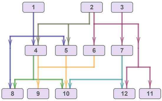
Figure 1.
An example of the layering of a hierarchical hypergraph with orthogonal hyperedges according to the accepted rules.
A well-known approach to hyperedge visualization is the replacement of each hyperedge with a set of edges with one dummy node, followed by the use of traditional layout techniques for graphs; then, the hypergraph is restored from the graph layout obtained in the previous step [3,4]. Therefore, this problem is closely related to hierarchical (i.e., directed acyclic) graph drawing, and methods based on the Sugiyama approach [5] will be applied.
To make this algorithm applicable to the hypergraph layout problem, Sander [6] first proposed reordering the nodes on each layer to minimize the number of edge crossings, and then calculated the preliminary coordinates for the nodes and segments to avoid hyperedge crossings, finally obtaining the coordinates that rendered a balanced drawing. In [7], an exact formulation of the mathematical problem of hyperedge routing was proposed, and it satisfied the constraints discussed above. The final step of the hypergraph drawing algorithm is assigning each upper vertical segment to a port of its source node and each lower vertical segment to a port of its target node.
Computing the optimal order of vertices for all layers of a graph is a highly time-consuming procedure. That is why it is reasonable to reorder vertices in each layer separately to minimize the number of edge crossings related to one of adjacent layers. A heuristic proposed in [8] was improved in further work; see [9].
Plenty of exact and heuristic algorithms have been presented for the minimization of edge crossings by reordering nodes on layers; see, e.g., [8,10]. However, application of these methods for a hypergraph might not provide acceptable results. It is known that decreasing the number of edge crossings does not ensure the same for the corresponding hypergraph [11]; see, for instance, Figure 2 and Figure 3, which present examples of single-source one-port hypergraphs.
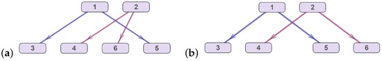
Figure 2.
Reordering nodes on the lower layer of a graph leads to a decrease in the number of edge crossings: two crossings for the layout (a) and one crossing for the layout (b).
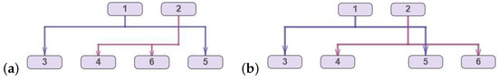
Figure 3.
The same reordering nodes on the lower layer of the corresponding hypergraph leads to an increase in the number of hyperedge crossings: one crossing for the layout (a) and two crossings for the layout (b).
An additional optimization problem arises if one takes ports for the source and target nodes into account because each vertical segment of a hyperedge must be assigned to a unique port. This problem should be considered as a part of a hierarchical hypergraph drawing problem, together with the reordering of nodes and horizontal segments. Figure 4 and Figure 5 show three layouts of the same hypergraph: without ports (optimal layout), with the assignment of ports as a result of a post-processing procedure, and, finally, with the optimal assignment of ports.
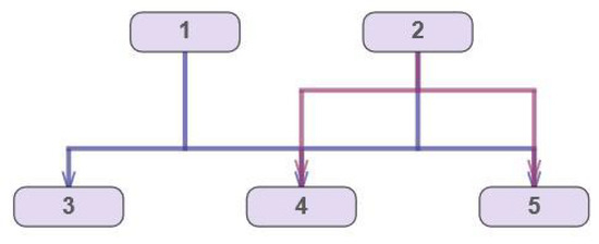
Figure 4.
Optimal layout of a hypergraph; no ports allowed.
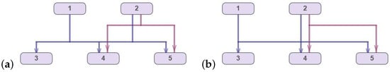
Figure 5.
Layout of a hypergraph with ports for the source and target nodes: (a) non-optimal layout; (b) optimal layout with ports.
The reordering heuristic by Eschbach et al. [12] only gives a local minimum of the number of hyperedge crossings. Spönemann et al. [11] proposed an algorithm for quite accurate (but not exact) counting of hyperedge crossings depending on the order of nodes without computing the hyperedge routing.
A hyperedge drawing is applied in a variety of practical areas: from cooperation scheme drawing and information and financial flow visualization to schematics of displays of automotive communication networks and VLSI design. Interesting applications of the hypergraph layout problem can be found in the development of effective routing protocols for IoT applications and in the development of energy-balanced routing protocols for terrestrial/underwater wireless sensor networks, as well as in the assessment of their safety.
The information system for the national investment projects that started in Russia in 2015 is an example of graphical data analysis [7]. One of the goals of this information system is to control all financial transactions and contracts related to large-scale national projects, in which hundreds of companies are involved. The embedded software visualizes companies as nodes of a hierarchical hypergraph and their business links and financial transactions as directed hyperedges. This visualization scheme enables one to highlight potential risks and to estimate the status of a project under consideration. It is clear that this visualization is only helpful as an analytical tool if it is easy to understand. It is more to the point that the hypergraph density is high.
The neighboring area of application is financial flow visualization for corporations with large numbers of branch offices and commercial subsidiaries. The display of the flow of information within or between universities can be discussed as an application as well.
There are some novel approaches to nanostructures and material science with application of graph theory [13,14], where there is a large variety of applications connected with hierarchical hypergraphs with orthogonal hyperedges.
2. Requirements for Hyperedge Drawing
In mathematical terms, a directed k-layering hypergraph contains a set V of nodes and a set of hyperedges. A hyperedge has source nodes and target nodes . A layering function is introduced in order to partition the set of vertices V into a k finite subsets (layers) . The function assigns a positive integer to each vertex (layer), .
We assume the following set of requirements for orthogonal hyperedge routing, which is complementary to that for a layered graph drawing [10]:
- Each hyperedge e consists of three elements: upper vertical segments , horizontal segments , and lower vertical segments ;
- Each hyperedge is incident to one or more source vertices and adjacent (target) vertices of the lower layers;
- Vertices are represented by rectangles of a fixed size with a set of ports on their upper and lower sides. In fact, every port is a common point of a vertex and an incident hyperedge;
- Each port of a vertex corresponds to exactly one vertical segment, either a segment of or a segment of . The number of ports of a vertex is equal to the number of incident hyperedges for this vertex;
- For every two hyperedges and , it holds that and intersect if and only if a horizontal segment has crossing points with a vertical segment, a segment of , or a segment of , or vice versa. Note that this requirement means that the overlapping of segments becomes non-feasible for hypergraph drawing. Two examples of such non-feasible overlapping are demonstrated in Figure 6;
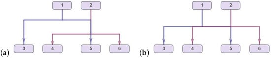 Figure 6. Examples of the non-feasible overlapping of hyperedges: (a) non-feasible overlapping of vertical segments; (b) non-feasible overlapping of horizontal segments.
 - The number of hyperedge crossings is to be minimized.
3. Mathematical Model for Drawing a Hierarchical Hypergraph with Orthogonal Hyperedges and Ports
If hypergraph H contains hyperedges connecting the vertices of non-adjacent layers, then every such “long” hyperedge e has to be transformed into several hyperedges that connect the vertices of adjacent layers only, with additional (dummy) vertices being introduced for every e in the following way:
- Find adjacent vertices u and v such that ;
- Insert a single dummy node on each layer l of hypergraph H, ;
- Replace the long hyperedge e with hyperedges that connect the inserted dummy vertices with the incident vertices of the original long hyperedge e so that each new hyperedge connects the vertices of the adjacent layers. This step should hold all of the connections between nodes on adjacent layers that are defined by hyperedge e.
Consider the hypergraph , which is constructed from the hypergraph H (after inserting dummy vertices into it) by splitting each vertex into subsets of port vertices. For each vertex (so-called “generating vertex”), sets and of the port vertices are introduced, and , where and denote the numbers of ports of vertex u for the upper vertical segments and for the lower vertical segments of the incident hyperedges, respectively. Each port vertex in the set is considered a vertex of hypergraph . A function C is introduced as well. For each port vertex, the function C yields its generating vertex. Note that . Figure 7 demonstrates an example of such a transformation of hypergraph H into hypergraph .
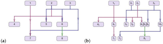
Figure 7.
Transformation of hypergraph H into hypergraph : (a) original hypergraph H; (b) hypergraph obtained after inserting dummy vertices and port vertices.
The following specific constraints are to be taken into account for the drawing of hypergraph : port vertices with the same value for function C (those generated by one generating vertex) should be neighboring ones, i.e., between any two port vertices with the same value for function C, on every layer, there is no port vertex with another value for function C.
For the mathematical formulation of the hypergraph drawing problem, three sets of real variables are introduced—X, , and —as well as four sets of integer variables—, , , and .
Variable denotes the x-coordinate of the vertex . The variables and are the x-coordinates of the leftmost and rightmost nodes of hyperedge e, respectively.
A minimum distance is known for each pair of port vertices : (or ), , or each pair of generating vertices : . The order relation for a pair of vertices u and v means that they are in lexicographic order on the same layer.
A maximum distance is known between each pair of port vertices (or ) of a generating vertex u, .
A minimum distance is known between vertical segments and or and for each pair of hyperedges : . The order relation for a pair of hyperedges and means that they are in lexicographic order, and their source vertices are on the same layer.
Each hyperedge has a so-called “area of crossings”. This can be defined as a set of points with coordinates such that and y is between the ordinates of the source and target nodes. Figure 8 demonstrates the area of crossings of hyperedge with the incident vertices . Vertices , which are incident to another hyperedge , are inside this region, and vertices 3 and 6 are outside of it.
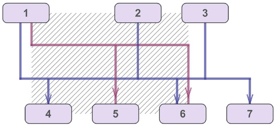
Figure 8.
The area of crossings of hyperedge .
For each pair of hyperedges with source vertices on the same layers, where , and , the integer variables and and dummy variables and are introduced as follows:
The variable is the number of crossings between the horizontal segment of one hyperedge of a corresponding pair of hyperedges and the upper segments of the other hyperedge. Similarly, the variable is the number of crossings between the horizontal segment of one hyperedge of this pair and the lower segments of the other hyperedge. The number of crossings for a pair of hyperedges and depends on the number of port vertices inside the area of crossings of these hyperedges and the relative vertical positions of their horizontal segments.
The following optimization criteria are applied in the model:
- Reducing the number of hyperedge crossings;
- Symmetric arrangement of source nodes relative to target nodes.
These can be formulated in the form:
Note that, in all of the formulae below, denotes the set cardinality for sets and an absolute value for numerical expressions.
To ensure that no vertices overlap in the hypergraph layout, the distance between every pair of generating vertices u and v on the same layer () should be equal to or greater than , i.e., . Taking into account that the abscissa of a generating vertex u can be calculated as the mean value of its port vertices with abscissas, we re-write this condition in the form
Analogous conditions are to be imposed for the distance between each pair of port vertices (or ) of every generating vertex . Note that they set both the minimum and the maximum distance between and as follows:
The next set of conditions ensure that the mean value of the x-coordinates of the port vertices in the sets and are equal such that all of the port vertices in and are to be merged back into one generating vertex in the hypergraph drawing:
The obvious condition that every port vertex u incident to hyperedge e lies between the leftmost and the rightmost vertices incident to hyperedge e defines the following connection between variables , , and for every hyperedge e:
A set of constraints (11)–(17) is formulated for each pair of hyperedges , with source nodes on the same layer.
If the abscissa of a port vertex u incident to the hyperedge belongs to the interval that is defined by the x-coordinates of the leftmost and the rightmost vertices incident to hyperedge , then the vertex u is inside the area of crossings of hyperedge . In this case, there might be a crossing of a vertical segment of hyperedge connected with the vertex u and a horizontal segment of hyperedge . The fact that a vertex is inside the area of crossings for a pair of hyperedges depends on the abscissa of the vertex and the values of the variables and in the following manner:
Note that in expression (11) and in all of the formulae below, M is an arbitrary large positive number, .
The vertical segments of every two hyperedges have no common point in the hypergraph layout. Hence, one has to ensure a minimum distance between the horizontal positions of the port vertices connected to these segments. The following conditions ensure the absence of non-feasible overlaps of hyperedge segments:
The transitivity condition is to be satisfied for the positions of the horizontal segments of any triplet of hyperedges:
Finally, we determine the domains for all of the variables in the problem:
The standard linearization procedure for nonlinear expressions (6)–(9), (11), (16), and (17) allows one to obtain a multi-objective mixed-integer program (5)–(21).
Figure 9 illustrates an example of the optimal layout of a hypergraph that was obtained on the basis of the model discussed above.
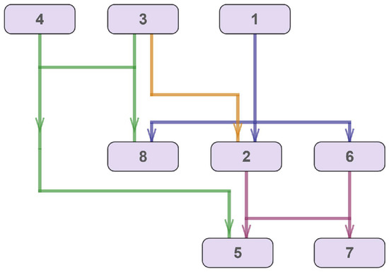
Figure 9.
An example of the optimal layout of a hypergraph.
Two additional post-processing steps are required for an optimal hypergraph layout: first, all dummy vertices must be rendered as points, and second, all subsets of the port vertices corresponding to a generated vertex must be merged back into one vertex.
4. Minimizing the Height of the Hypergraph Drawing
The optimization model in (5)–(21) yields the relative order of the horizontal segments of the hyperedges. Clearly, some horizontal segments can be placed on the same horizontal level of the hypergraph layout without non-feasible overlapping. The smaller the number of horizontal levels where the horizontal segments are placed, the smaller the height of the hypergraph drawing will be.
Some modifications of the model in (5)–(21) are considered to minimize the number of horizontal levels for the horizontal segments of hyperedges.
First, two types of additional variables are introduced: real variables Y and binary variables .
The variables are defined for each pair of hyperedges and so that in the following way:
The variables determine the relative level for the horizontal segment of every hyperedge . The smaller the value of is, the higher the horizontal segment of hyperedge e will be in the hypergraph drawing.
Conditions (23) and (24) are formulated for each pair of hyperedges and with source nodes on one layer, and they ensure that the values of and differ by a positive integer if the corresponding horizontal segments are on different levels. Again, a constant is used.
Figure 10 shows an example of the optimal layout of the hypergraph obtained using the described variant of the model. The horizontal segments of some hyperedges have the same ordinate, which makes it possible to reduce the height of the figure.
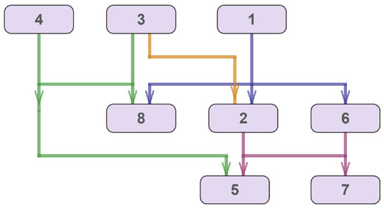
Figure 10.
An example of the optimal layout of the hypergraph with the same ordinates of horizontal segments.
5. A Mathematical Heuristic for the Hypergraph Layout
The problem of the hypergraph layout in (5)–(21) can be solved using the following five-step mathematical heuristic:
- Find the order of the vertices on each layer;
- Assign preliminary abscissas to the vertices;
- Find the relative order of horizontal segments for orthogonal hyperedges with source nodes on the same layer;
- Remove the non-feasible overlapping of vertical segments;
- Assign ports to the vertical segments.
Note that the aesthetic criteria used in the heuristic coincide with those in Section 3. The mathematical heuristic is sketched below; see Algorithm 1.
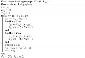
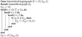
| Algorithm 1: A mathematical heuristic for the hypergraph layout. |
Data: hierarchical hypergraph |
Result: hypergraph drawing D |
; |
; |
; /∗ (26)–(30) ∗/ |
; |
; /∗ (31)–(33) ∗/ |
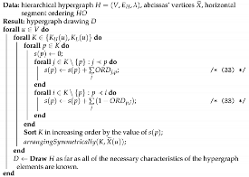
The first step (vertex ordering) includes a pre-processing procedure for the initial hypergraph H; the corresponding function is denoted as in Algorithm 1. A detailed description of this function that returns a graph corresponding to hypergraph H is given in Algorithm 2.
| Algorithm 2: The function. |
 |
To convert the hypergraph into a graph with the function, the so-called “balancing vertex” is introduced for each hyperedge ; see Figure 11a,b. Then, each vertex incident to the hyperedge is connected by a directed edge to the balancing vertex. This approach enables one to correctly take into account all possible intersections of edges.
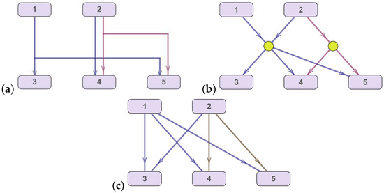
Figure 11.
An example of a hypergraph transformation: (a) original hypergraph H; (b) restructuring a hypergraph into a directed graph with balancing vertices; (c) restructuring a hypergraph into a directed graph.
The order of the vertices on the layers from is determined using the function; see Algorithm 1. The vertex-ordering problem is solved using an integer program [10] that minimizes the number of edge crossings in a directed acyclic graph.
To assign preliminary abscissas to the vertices (step 2 of the mathematical heuristic), the function is used. Again, hypergraph H is pre-processed with the function; see Algorithm 3. As a result of the transformation, every pair of adjacent vertices on the adjacent layers is connected by a directed edge; see Figure 11c.
| Algorithm 3: The function. |
 |
Then, x-coordinates are assigned to the vertices based on the solution to a linear programming problem with objective function (6); see [9]. Note that the relative vertex order on each layer remains.
Once step 2 is over, three introduced functions—, remove-Overlapping, and —are applied to obtain the hypergraph drawing. These functions correspond to steps 3, 4, and 5 of the mathematical heuristic, and their detailed description is presented below.
Knowing the x-coordinates of the vertices, the order of the horizontal segments of the hyperedges is determined. The objective function L that is minimized in step 3 is the number of hyperedge crossings:
For each pair of hyperedges and , one can calculate the number of source nodes and target nodes that are inside the area of crossings of hyperedge . We denote these numbers as and , respectively. Then, the system of constraints for the integer programming problem with objective function (26) is as follows:
Constraints (27) and (28) are a simplified version of conditions (12)–(15) from the optimization model described in Section 3. The simplification is based on the fact that the x-coordinates of vertices are known. Expression (29) coincides with condition (18) and ensures that the transitivity condition is satisfied for the positions of the horizontal segments of any triplet of hyperedges. Condition (30) determines the domains of all of the variables in the problem.
The function —see Algorithm 1—is the solution to the mixed-integer program in (26)–(30). It returns the relative order of horizontal segments of the hyperedges.
In step 4, all non-feasible overlaps of vertical segments of hyperedges are removed by using the integer program proposed in [7]. This solution is denoted as the removeOverlapping function in Algorithm 1. Non-feasible overlaps must be eliminated by shifting the vertices on layers by a certain integer number of “single shifts” for each corresponding vertex x-coordinate while maintaining the relative order of the vertices on the layers. The objective function of the integer programming problem minimizes the total number of shifts of vertices, and the constraints are (7)–(21) with fixed values of the variables for every pair of hyperedges.
The last step of the mathematical heuristic is the port assignment procedure when the relative order of ports is determined by the function for each hypergraph vertex—see Algorithm 4—where the function determines the x-coordinates of the port vertices by placing them symmetrically to the x-coordinate of the generating vertex without breaking the relative order of the port vertices.
| Algorithm 4: The function. |
 |
For every generating vertex u, binary variables are introduced for each pair of port vertices or (relation holds) as follows:
A numerical parameter is defined for each pair consisting of a hyperedge and a generating vertex :
Consider a pair of a hyperedge and a generating vertex . If , then u is the leftmost vertex in a set of vertices incident to e, and if , then u is the rightmost one. The equality means that vertex u is between the leftmost and the rightmost vertices incident to e. Parameter enables one to define the value of , i.e., the relative order of two port vertices u and v, as follows:
where denotes the unit step function, u and v are incident to the hyperedges and , respectively, or , , and a numerical parameter takes the value 2 if port vertex u for the upper vertical segment of or 1 in the other case.
Once the relative order of all pairs of port vertices , is known, all of the port vertices of the generating vertex u are positioned so that their mean x-coordinate coincides with that of the center of u. The minimal and maximal distances and (see Section 3) should be taken into account. Figure 12 illustrates a hypergraph layout that was obtained using the mathematical heuristic approach described above.
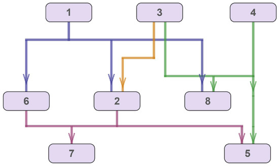
Figure 12.
An example of layout of a hypergraph obtained with the mathematical heuristic.
6. Numerical Results and Discussion
The approach to a solution of the hypergraph drawing problem proposed above was verified using synthetic initial data. The corresponding numerical results were analyzed for the multi-objective mixed-integer program in (5)–(21) and the mathematical heuristic (see Section 5) for a set of generated hypergraphs.
Wolfram Mathematica 12.3 [15] was used as a programming tool together with Gurobi Optimizer 9.1 [16]. All the numerical calculations were performed on an HP desktop, with an Intel Core i5 1.60 GHz CPU, 8 GB of RAM, and the Windows 10 operating system. The numerical results are presented in Table 1.

Table 1.
Numerical results obtained using the mathematical heuristic (MH) and mixed-integer program (MIP) for a set of generated hypergraphs.
Three approaches were applied to obtain the numerical results, namely, the mathematical heuristic (see Section 5), mixed-integer program (5)–(21) with a higher priority of the objective function (5), and the same mixed-integer program enhanced by an initial feasible solution derived with the mathematical heuristic approach.
Each hypergraph is described by its ID. If the ID contains the prefix ms, then the hypergraph is considered to have multi-source hyperedges; otherwise, all the hyperedges in the hypergraph are single-source ones (prefix ss in the ID). The numbers of vertices and hyperedges are indicated in the column (,). The column “Time in sec” gives information on the computation time for each numerical experiment. There is additional information (in parentheses) on how long it takes for Gurobi to find a solution that cannot be optimized with further iterations.
7. Conclusions
A new mathematical model for drawing a hierarchical hypergraph with vertex ports and multi-source orthogonal hyperedges is discussed in this paper. The model is based on the formulation of a mixed-integer program. One of the advantages of the model is that it enables one to simultaneously take into account a set of optimization criteria, including aesthetics ones (for overall hypergraph drawing), as well as the minimization of hyperedge crossings. The numerical results demonstrate that the number of hyperedge crossings can be minimized compared to the mathematical heuristic approach.
One of the application areas of the model is in financial flow visualization in information systems to create an initial drawing of a hypergraph. The initial layout is corrected when actual data are updated using the dynamic hierarchical graph-drawing algorithm [9].
Further directions of research include:
- The generalization of the proposed mathematical model for reverse-directed hyperedges by adding port vertices to the model on the left and right sides of the generating vertices;
- The development of a fast and efficient algorithm (heuristic, metaheuristic, column generation, etc.) for drawing large-scale hypergraphs.
Author Contributions
Conceptualization, G.F. and Y.V.; methodology, Y.V.; software, V.P.; validation, V.P.; formal analysis, G.F.; investigation, G.F., Y.V. and V.P.; resources, V.R.; data curation, G.F.; writing—original draft preparation, V.P.; writing—review and editing, G.F. and Y.V.; visualization, V.P.; supervision, G.F.; project administration, V.R.; funding acquisition, V.R. All authors have read and agreed to the published version of the manuscript.
Funding
The research was partially funded by the Ministry of Science and Higher Education of the Russian Federation as part of the World-Class Research Center program: Advanced Digital Technologies (contract No. 075-15-2020-903 dated 16.11.2020).
Institutional Review Board Statement
Not applicable.
Informed Consent Statement
Not applicable.
Data Availability Statement
Collection of the hypergraphs generated: https://drive.google.com/drive/folders/1GQL3gKQsVoDMrAt-YkHCYhaBabM7wBN- (Accessed: 14 December 2021). Additional data presented in this study are available on request from the authors.
Conflicts of Interest
The authors declare no conflict of interest. The funders had no role in the design of the study; in the collection, analyses, or interpretation of data; in the writing of the manuscript, or in the decision to publish the results.
References
- Spönemann, M. Graph Layout Support for Model-Driven Engineering; BoD–Books on Demand: Norderstedt, Germany, 2015. [Google Scholar]
- Helmke, S.; Goetze, B.; Scheffler, R.; Wrobel, G. Interactive, Orthogonal Hyperedge Routing in Schematic Diagrams Assisted by Layout Automatisms. In Diagrammatic Representation and Inference. Diagrams 2021; Lecture Notes in Computer Science; Springer: Berlin/Heidelberg, Germany, 2021. [Google Scholar] [CrossRef]
- Schulze, C.D.; Spönemann, M.; von Hanxleden, R. Drawing layered graphs with port constraints. J. Vis. Lang. Comput. Issue Diagr. Aesthet. Layout 2014, 25, 89–106. [Google Scholar] [CrossRef]
- Jünger, M.; Mutzel, P.; Spisla, C. More Compact Orthogonal Drawings by Allowing Additional Bends. Information 2018, 9, 153. [Google Scholar] [CrossRef] [Green Version]
- Sugiyama, K.; Tagawa, S.; Toda, M. Methods for visual understanding of hierarchical system structures. IEEE Trans. Syst. Man Cybern. 1981, 11, 109–125. [Google Scholar] [CrossRef]
- Sander, G. Layout of Directed Hypergraphs with Orthogonal Hyperedges. Graph Draw. 2003, 381–386. [Google Scholar] [CrossRef] [Green Version]
- Vasiliev, Y.M.; Fridman, G.M. Cooperation scheme visualization: Hyperedge routing method for hierarchical multilayer hypergraph. Sovrem. Ekon. Probl. Resheniia 2017, 3, 18–33. (In Russian) [Google Scholar] [CrossRef]
- Junger, M.; Mutzel, P. 2-layer straightline crossing minimization: Performance of exact and heuristic algorithms. J. Graph Algorithms Appl. 1997, 1. [Google Scholar] [CrossRef]
- Ismaeel, A.A.K. Dynamic Hierarchical Graph Drawing. Ph.D. Thesis, Karlsruher Instituts fur Technologie (KIT), Karlsruhe, Germany, 2012. [Google Scholar]
- Healy, P.; Nikolov, N.S. Hierarchical drawing algorithms. In Handbook on Graph Drawing and Visualization; CRC: Boca Raton, FL, USA, 2013; pp. 409–453. [Google Scholar]
- Spönemann, M.; Schulze, C.D.; Rüegg, U.; von Hanxleden, R. Counting Crossings for Layered Hypergraphs. In Diagrammatic Representation and Inference. Diagrams 2014; Lecture Notes in Computer Science; Springer: Berlin/Heidelberg, Germany, 2014; p. 8578. [Google Scholar] [CrossRef]
- Eschbach, T.; Guenther, W.; Becker, B. Orthogonal hypergraph drawing for improved visibility. J. Graph Algorithms Appl. 2006, 10, 141–157. [Google Scholar] [CrossRef]
- Šuvakov, M.; Andjelković, M.; Tadić, B. Hidden geometries in networks arising from cooperative self-assembly. Sci. Rep. 2018, 8, 1–10. [Google Scholar] [CrossRef] [Green Version]
- Tadić, B.; Andjelković, M.; Šuvakov, M.; Rodgers, G.J. Magnetisation Processes in Geometrically Frustrated Spin Networks with Self-Assembled Cliques. Entropy 2020, 22, 336. [Google Scholar] [CrossRef] [PubMed] [Green Version]
- Wolfram Research. Wolfram Mathematica. Available online: https://www.wolfram.com/mathematica/ (accessed on 14 December 2021).
- Gurobi Optimization, LLC. Gurobi Optimizer. Available online: https://www.gurobi.com/products/gurobi-optimizer/ (accessed on 14 December 2021).
Publisher’s Note: MDPI stays neutral with regard to jurisdictional claims in published maps and institutional affiliations. |
© 2022 by the authors. Licensee MDPI, Basel, Switzerland. This article is an open access article distributed under the terms and conditions of the Creative Commons Attribution (CC BY) license (https://creativecommons.org/licenses/by/4.0/).