1. Introduction
The principal problem of managing any objects in conditions of non-stationarity, non-uniformity, and/or chaotic dynamics is the lack of repeatability, which obstructs the use of conventional statistical research techniques. In this case, statistical extrapolation, which is the basis of automatic generation of management decisions, turns out to be ineffective, or even inapplicable [
1,
2,
3]. Hence, there is a need to search for regularizing effects that stabilize (at least locally) the prediction process in a given range of changes in the values of characteristic parameters.
This research considers a multidimensional time series of current readings of a number of financial instruments that evaluate, each from its own viewpoint, a certain market asset. The current market value of an asset is monitored based on the readings of the corresponding instrument. These readings can be adjusted, taking into account other similar instruments. In principle, all readings have a common base and are mutually correlated. The hypothesis is that the system of correlations between instruments has a significant degree of inertia [
4,
5,
6] and is approximately preserved with a small time lag.
Within the framework of this article, correlations between quotations of instruments are used as a regularizing mechanism. Similarly to other probabilistic characteristics of observation series, the parameters of the relationship change over time, which corresponds to the non-stationarity of the observed processes. However, the variability in correlations is significantly lower than that of the initial quotation changes. Moreover, with the growth of the observation window used to estimate the relationship parameters, the correlation characteristics stabilize near asymptotically stable values.
Hence, an assumption arises about the possibility of using these relationships to build multi-regression indicators that reflect market estimates of the current value of financial instruments. The mismatch of the market estimate of an instrument with its current value allows us to obtain an idea of the further dynamics of its quotation, which, as a rule, approaches equalizing the value of the instrument in relation to the “fair” market price. This, in turn, creates the basis for building a proactive management strategy based on this discrepancy.
It would be irrational to evaluate the quality of forecasting in conditions of market chaos using conventional indicators of the effectiveness of statistical estimates due to the above-mentioned features of the considered observation series. Rather, the effectiveness of such estimates should be assessed via terminal performance indicators of management strategies based on them. The corresponding numerical studies are provided in this paper.
This article is structured as follows.
Section 2 contains the main conceptual research contributions of this work. It presents quotation data on several financial instruments, which demonstrate that they are highly correlated. Further on, it contains a detailed description of the proposed problem, a basic asset management strategy that is based on corrected estimates of a selected indicator. Next, the task specifics that decrease the effectiveness of traditional statistical methods are considered as well as the approaches to improving the estimate quality via selecting the indicator kernel and removing some of the outliers.
Section 3 contains the resulting scheme for correcting estimates using an evolutionary algorithm. Finally,
Section 4 and
Section 5 are dedicated to a discussion and our conclusions, respectively.
2. Analyzed Data and Methodology
2.1. Data Model
Papers [
7,
8,
9,
10] justify describing quotation observation series on the basis of the Wald theorem by an additive model
where x
k, k = 1, …, n is a smoothed system component used for constructing management strategies and v
k, k = 1, …, n is noise. Similarly, instead of y
k, first finite differences of their logarithms could be used (i.e., the ARCH or GARCH models) [
11,
12], but this complicates returning to an estimation of the initial y
k. Let us highlight two important features of the presented observation model:
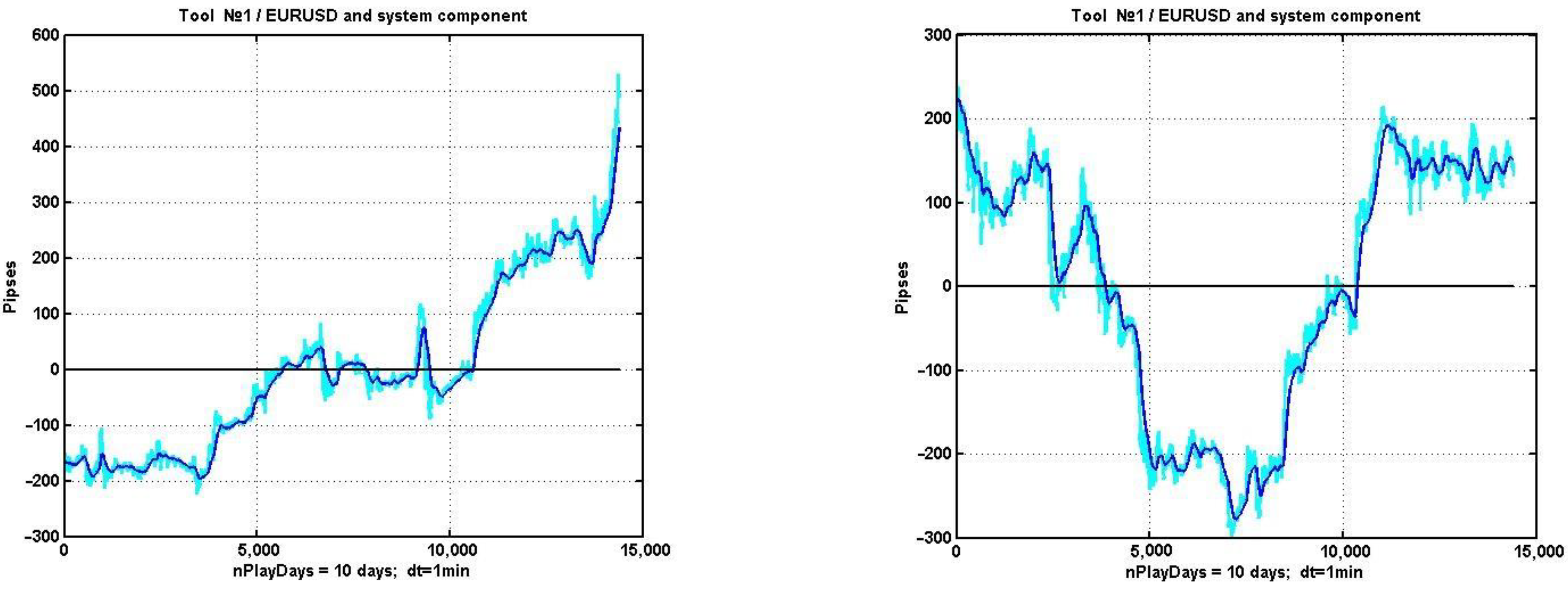
As illustrations justifying the choice of the model,
Figure 1 shows examples of quotations of financial assets on 10-day observation intervals.
To isolate the system component, an exponential filter
with a smoothing coefficient α = 0.01–0.3 was used.
The observed process y
k, k = 1, …, n does not conform to the efficient market hypothesis [
7] and, as shown in [
16,
17], has almost no inertia. The latter statement leads to a complete failure of management strategies based on mechanistic prolongation of the detected trends. At the same time, useful patterns can also be found in the system of correlations of trading asset quotations, as they are represented by multivariate observation series. In particular, increasing the observation interval makes it possible to detect stable correlations between various instruments of the currency and other markets [
18,
19].
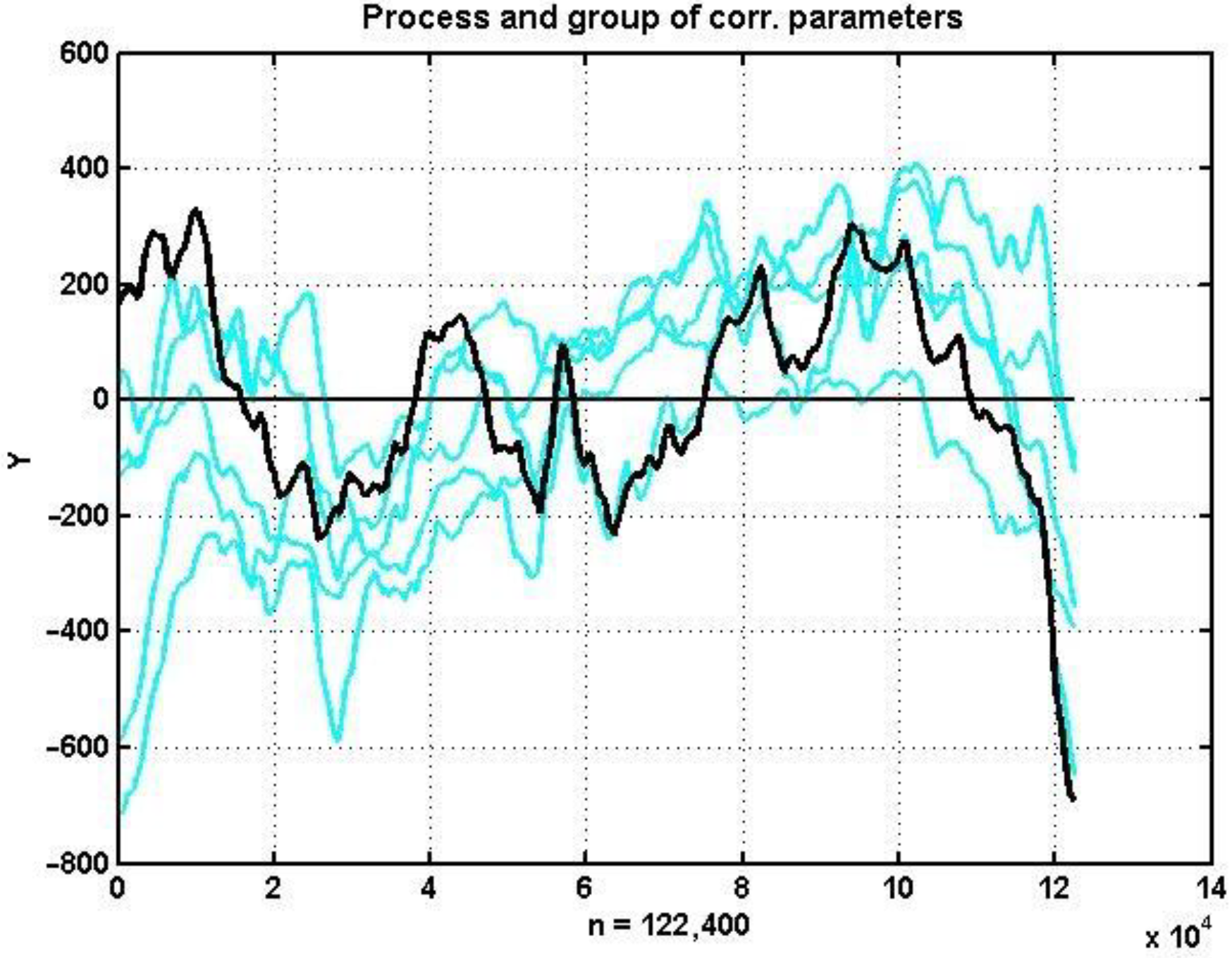
As an example illustrating the last statement,
Figure 2 shows time-synchronized charts of quotations of five different currency instruments on an 85-day observation area.
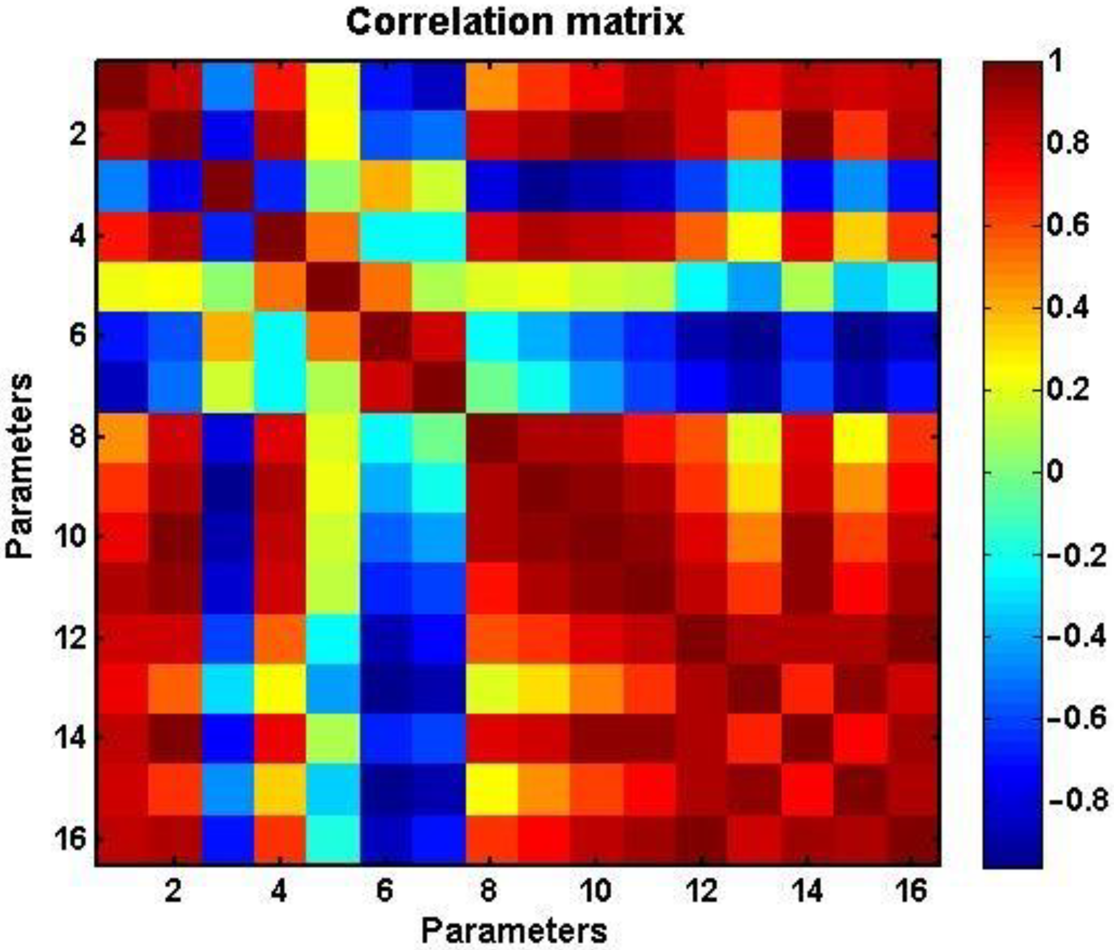
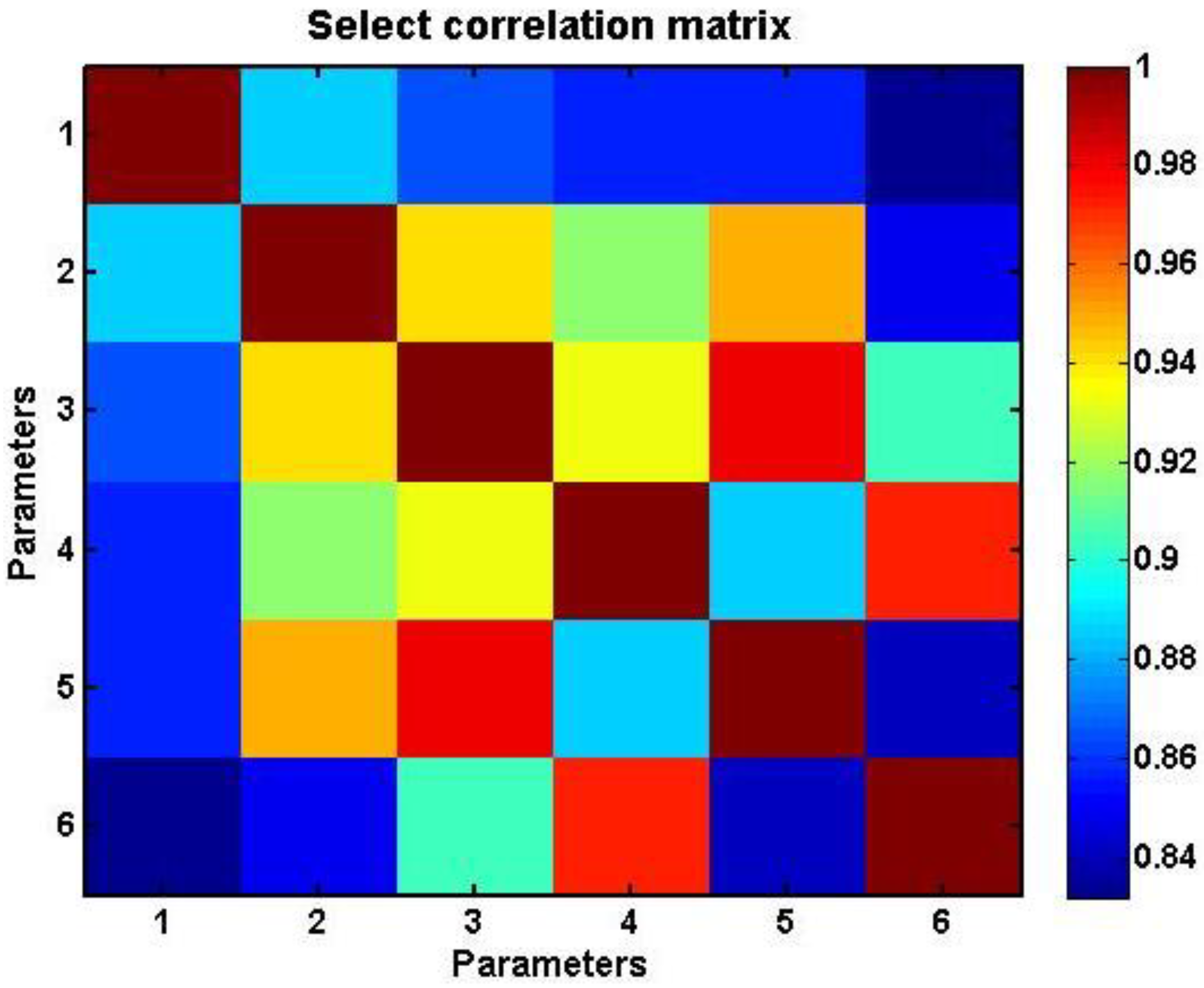
Figure 3 shows a tonal matrix reflecting the values of estimated pairwise correlations in the same observation interval for 16 currency pairs presented in
Table 1.
Figure 4 shows a similar tonal matrix for the pairwise correlations of EURUSD and its five most correlated currency pairs (#11: GBPUSD, #14: CHFJPY, #16: NZDJPY, #2: EURJPY, and #12: AUDJPY). These exact instruments are plotted in
Figure 2.
The presence of ordered relationships with lower variability than the quotes of working assets themselves allows us to construct mutual statistical dependencies, which, in turn, make it possible to adjust the current value of a financial instrument using its correlated instruments. Hence, there is a real possibility of constructing management strategies based on a statistical indicator, the value of which at any given time will be determined by the difference between the current quotation of a currency instrument and its estimate based on a group correlated with it. The most natural way of constructing such a forecast is multivariate linear regression (multi-regression) based on the modifications of the least squares method (LSM) [
20,
21].
It is obvious that the difference between the estimate and the current quotation of an asset can be used to manage assets with a variety of criteria that determine the time of opening and closing positions during the trading process. At the same time, in conditions of non-linearity and non-stationarity, analytical methods for comparing these criteria cannot be implemented. Hence arises the problem of numerical research on analytic and management techniques based on multi-regression (MR) estimation of a currency instrument, which is considered in this article.
2.2. Problem Statement
We consider a number of observations of the value of a non-stationary random process described by model (1), the system component of which is an oscillatory non-periodic process classified as deterministic chaos. On the same observation interval, an m-dimensional non-stationary random vector process is present, the elements of which are correlated with (1) and correspond to the same model of stochastic dynamics
As a result of numerical experiments, it was found [
18] that in general, among a set of financial instruments, it is possible to choose a vector subset (3) that has a significant correlation with the working (i.e., used in financial transactions) instrument y
k, k = 1, …, n. In the future, the elements Y
R will be used as regressors in the traditional MR model
The most natural way to estimate the value of the transfer coefficient C
k, k = 1, …, n, as already noted, is via the use of a conventional computational scheme based on the LSM:
All data accumulated during the observation from 1 to k − 1 are initially used as a training sample.
The analysis of the condition of a working tool consists in assessing the significance of the discrepancy between its current value y
k, k = 1, …, n and its regression estimate (4), reflecting the opinion of the market, represented by a set of regressor instruments, about its real value. If the regressors are representative in terms of their ability to reflect significant market variations, then the difference
will reflect the degree of under- or overpricing of the selected working instrument. This directly implies recommendations for a management strategy: the opening of a position should be carried out in a direction that compensates for the resulting fluctuation discrepancy (6).
2.3. A Simple Management Strategy Based on Multiregression Estimation
Despite the validity and constructiveness of the considered forecasting and management technique, the solution of this problem faces a number of significant issues due to the specifics of the data model (1). Let us consider this question in more detail.
The simplest asset management strategy based on computational regression estimates can be constructed upon criterion K: |dk| > d*, k = 1, …, n. If dk > d*, this means that ŷk > y + d*, i.e., the financial instrument is underpriced, and its price can be expected to go up. Vice versa, dk < −d* indicates an overprice, and therefore the instrument’s price should be expected to go down.
The conventional statistical approach involves determining the critical value d* based on its distribution tables (or the distribution of an associated statistic) and a given level of confidence. In the conditions of non-stationary dynamics with a chaotic systemic component, such an approach is unfeasible. The critical value has to be selected based on preliminary analysis of retrospective information drawn from a large observation interval.
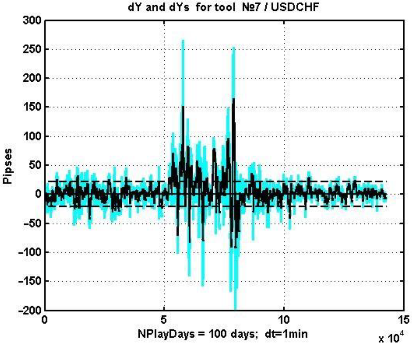
As an example, let us consider the change in (6) for USDCHF on a 100-day observation interval with a 5-min step. The respective plot, its smoothed version, and the decision levels are presented in
Figure 5.
The threshold value d* for making a management decision is the standard deviation (SD) of dk estimated on the selected observation interval. The corresponding estimate of the SD of the difference process was s = 24.7 and s = 21.5 for the smoothed process.
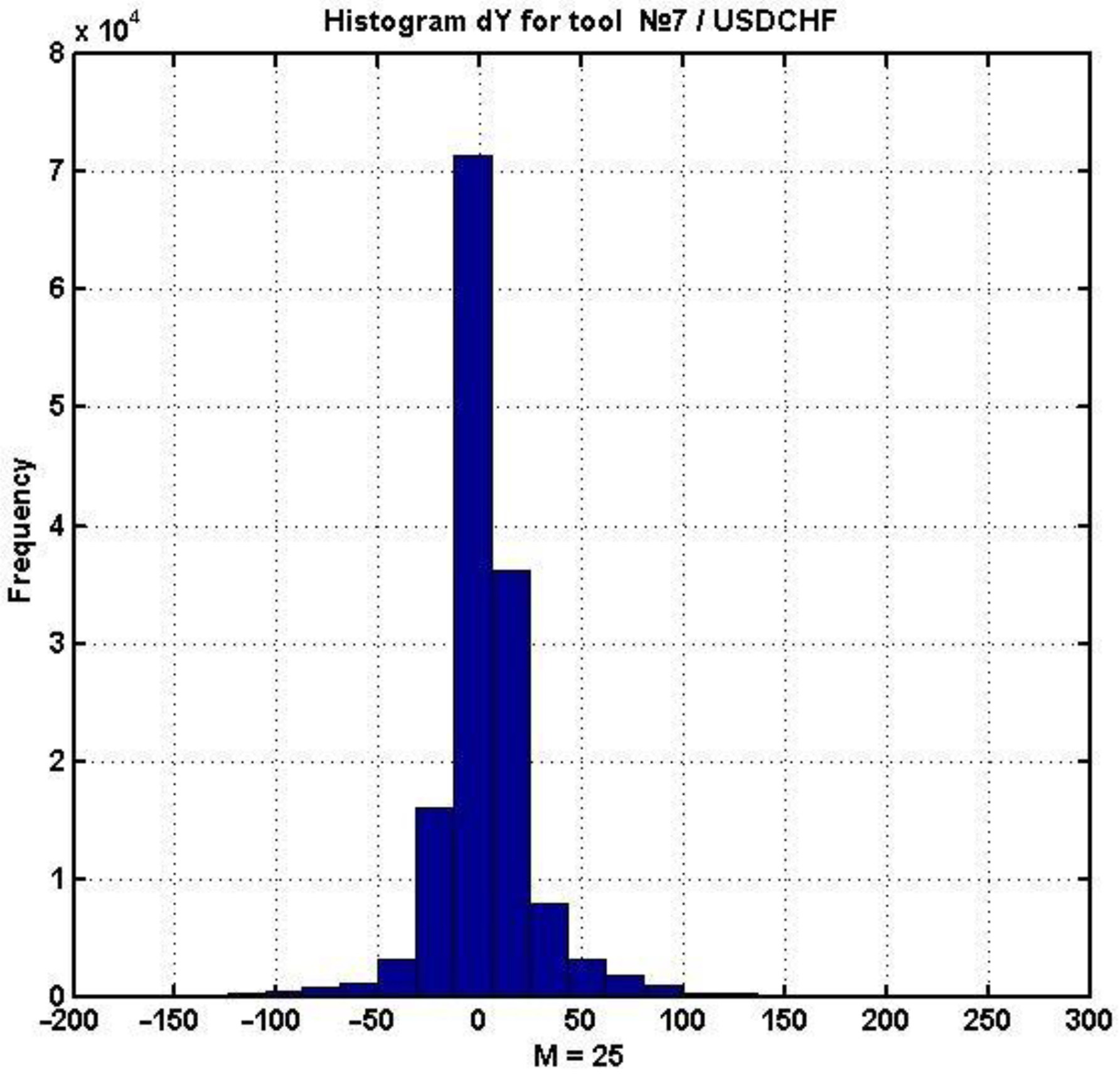
Figure 6 contains a histogram of d
k, k = 1, …, n, which demonstrates the weak convergence of the given difference’s distribution to the Gaussian law. This picture is static; considering it dynamics-wise, it can be seen that all the moments of the distribution change over time, and therefore the process is purely non-stationary.
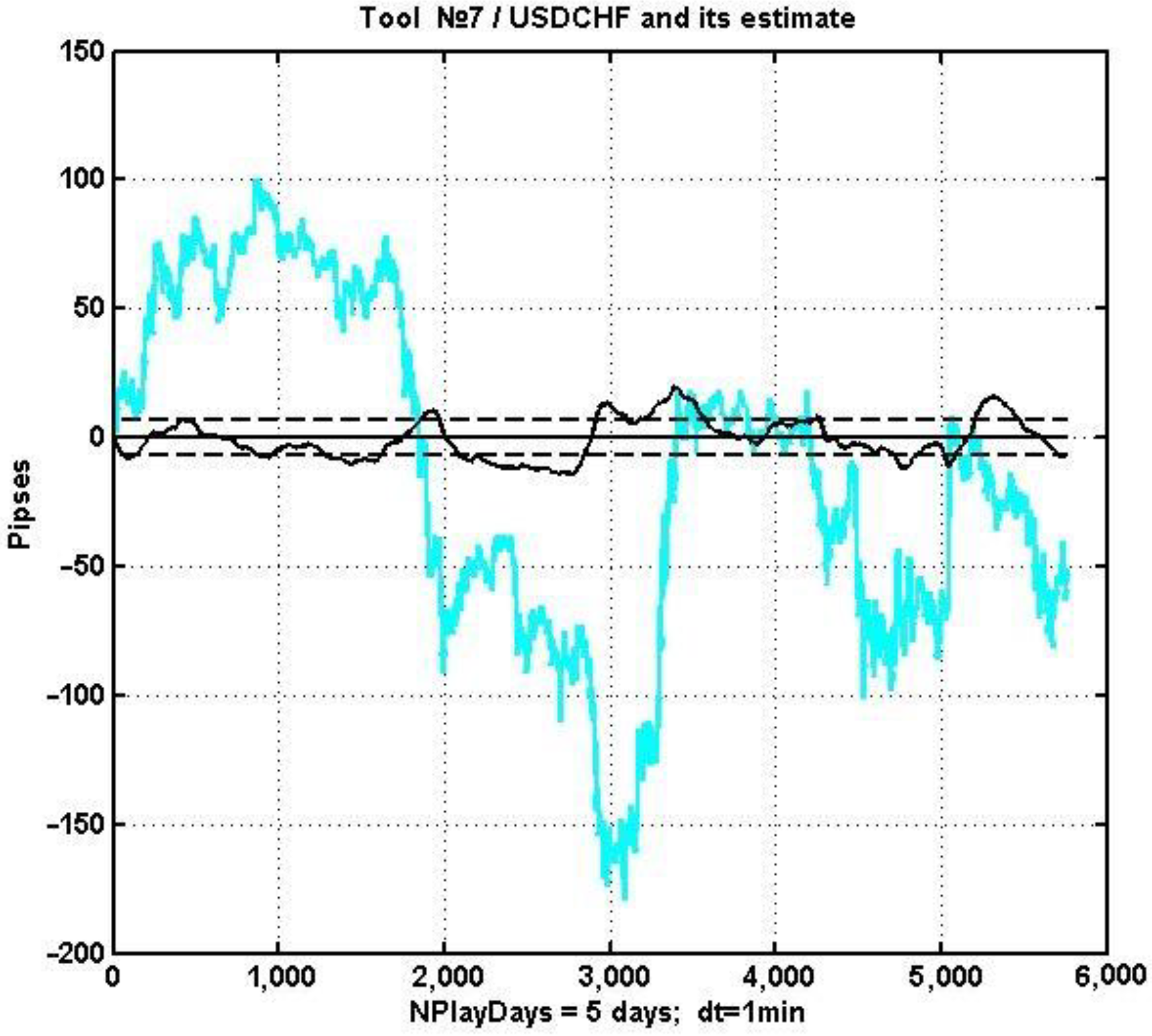
Next, let us consider the combined plots of the initial process and the criterion statistics (an oscillator) d
k, k = 1, …, n (
Figure 7). For easier visualization, a relatively small observation interval (5 days) is considered, and the oscillator and its critical value are enlarged by 1.5 times.
According to the described management strategy, if the smoothed oscillator surpasses the threshold value, i.e., dk > d*, a long position should be opened. Alternatively, one can open a short position if dk < −d*. Positions can be closed along with a reverse crossing of the threshold d*, or by the conventional methods of setting Take Profit and Stop Loss levels.
Figure 7 shows that there is no stable trend for either underprice or overprice in this particular example. One can assume that, on a sideways (“flat”) trend, the multi-regression oscillator will work quite effectively with correctly selected values of the management strategy’s parameters. However, if there is a strong trend caused by factors external to the market, the corresponding trend will prevail, majoring the influence of the discrepancy between the current price of the asset in relation to its market value.
Thus, in order to construct an effective management strategy based on the discrepancy between the asset price and its market estimate in conditions of non-linearity and non-stationarity, it is necessary to form a set of regressors most associated with the working instrument for the current short observation interval. This approach involves structural adaptation of the MR model (4), which in turn requires a more careful study of the features of the estimation task in the conditions of non-stationary dynamics of market parameters.
2.4. Specifics of Financial Instrument Value Analysis in the Conditions of Non-Stationary and Non-Linear Dynamics
The traditional MR estimation meets the conditions of non-bias, consistency, and asymptotic efficiency only when a number of constraints are met. Let us describe some of them:
The system component of a series of observations (1) xk, k = 1, …, n is an unknown deterministic process, which in some cases can be expressed analytically;
Regressors are not mutually correlated, i.e.,
The noise component of the model (1) v
k, k = 1, …, n is stationary, centered relative to the system component, and uncorrelated to the regressor’s random process
The simplest methods of data analysis based on algorithms of statistical hypothesis testing show that real observation series obtained via monitoring values of market assets do not fully meet the constraints listed above. This means that the price estimates of the working instrument obtained via statistical analysis are not only not optimal, but also, as a rule, are biased. At the same time, it is not possible to construct analytical methods for calculating a market estimate of a financial instrument for a model of type (1). Thus, the main method of analyzing the quality of evaluation, as has already been noted, is computational studies.
One of the known ways to reduce the bias of statistical estimates for non-stationary processes is to limit the length of the series of observations via a sliding observation window
, where
, and L is the window size. At the same time, the most up-to-date data should be processed, reflecting the current situation to a greater extent. The multipliers in the estimation algorithm using the LSM (5) are given by expressions
The size of the observation window is usually chosen to minimize the mean square of the error L*: d2 = s2 + b2 = min(L), where s is the estimate of the SD, and b is the estimated bias. However, for a model of the form (1) with a chaotic system component, it is not possible to obtain stable estimates of SD and bias values. In this regard, the choice of the observation window is carried out empirically, by comparing the estimation results on the training observation window preceding the current time.
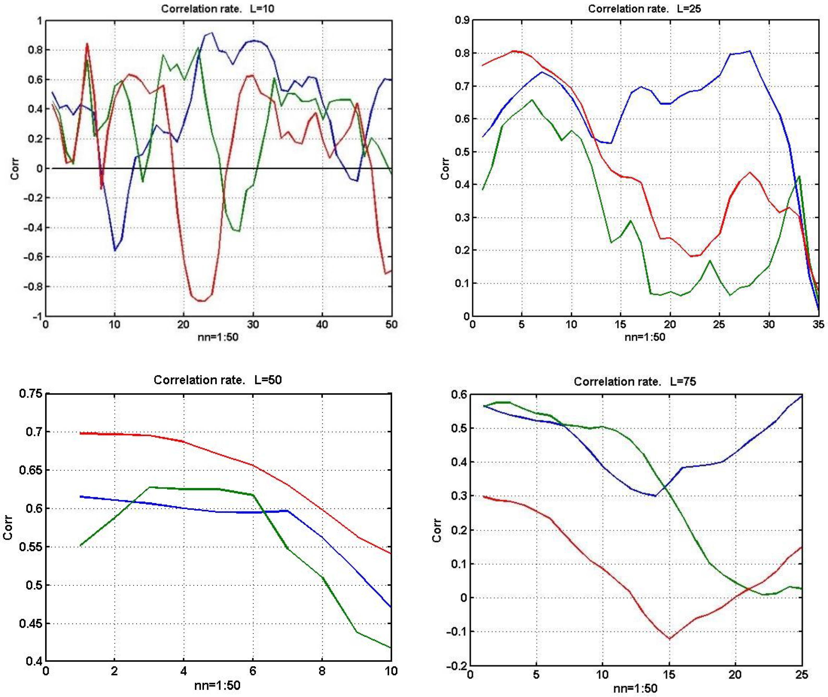
Another important feature of the statistical analysis of financial instruments is the presence of significant variations in the correlation matrix of the used regressors.
Figure 8 shows changes in the estimates of the pairwise correlation between two correlated currency instruments with an increasing sliding observation window of size L = 10, 25, 50, and 75 counts, respectively.
It is not difficult to see that as the sample size increases, the estimates become more stable. However, for a current assessment of the value of a financial instrument, the best composition of regressors YRk, k = 1, …, n in the computational scheme (4) will be different at each time moment. This justifies the use of structural adaptation of the MR model with a step-by-step selection of financial instruments used as regressors.
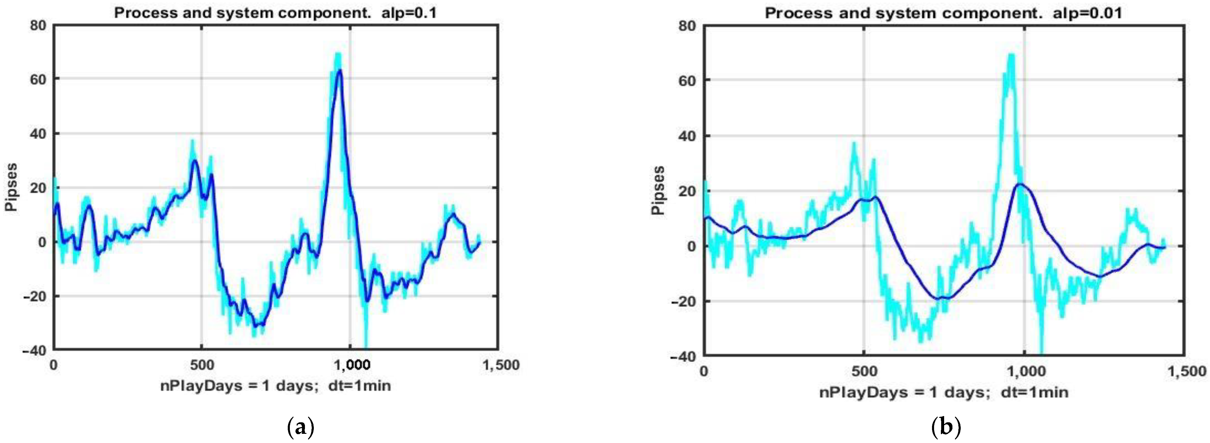
Another important feature of the considered problem is the separation of the system component from the initial process (1). In real time, this procedure is carried out by sequential filtering methods of type (2). It is quite obvious that an increase in the memory size of the filter or the weight characteristics of already smoothed observations leads to a decrease in the noise level v
k, k = 1, …, n. At the same time, this approach inevitably leads to delays in the reaction of current estimates to significant changes in the relative dynamics of quotations of financial instruments. In other words, there is a contradiction between the quality of smoothing random fluctuations in observations and the growth of the estimation bias caused by dynamic errors. An illustration of this problem is given by the example of the allocation of the system component of the quotes of the EURUSD currency pair using the exponential filter (2) for the filter coefficients
(
Figure 9a) and
(
Figure 9b).
Thus, the quality of recovery of the system component in data model (1) is determined by the compromise between the values of statistical and dynamic estimation errors. Furthermore, the shift in the balance between them depends either on the filter coefficient α (for a filter of type (2)) or on the size of the filter memory [
22]. In the conditions of chaotic dynamics described by model (1), the choice of this parameter also has no analytically sound recommendations and is based on empirical fitting to the results of retrospective analysis on previous observation segments that serve as a dataset. Double exponential filtration (back and forth) with α decreased to minimize bias could be a reasonable variant.
Based on the studies presented above, it can be concluded that the nature of the considered series of observations is deeply inconsistent with the known limitations of statistical analysis, which makes it possible to obtain effective estimates. Hence, an incorrect task of constructing management strategies arises in conditions when the quality of assessments of the state of market parameters is very uncertain. Traditional approaches to obtaining stable results in such situations are most often based on the principles of adaptation of estimates. The question of how this technique can be useful in conditions of chaotic dynamics remains open. Some aspects of this problem are touched upon in this article.
3. Results
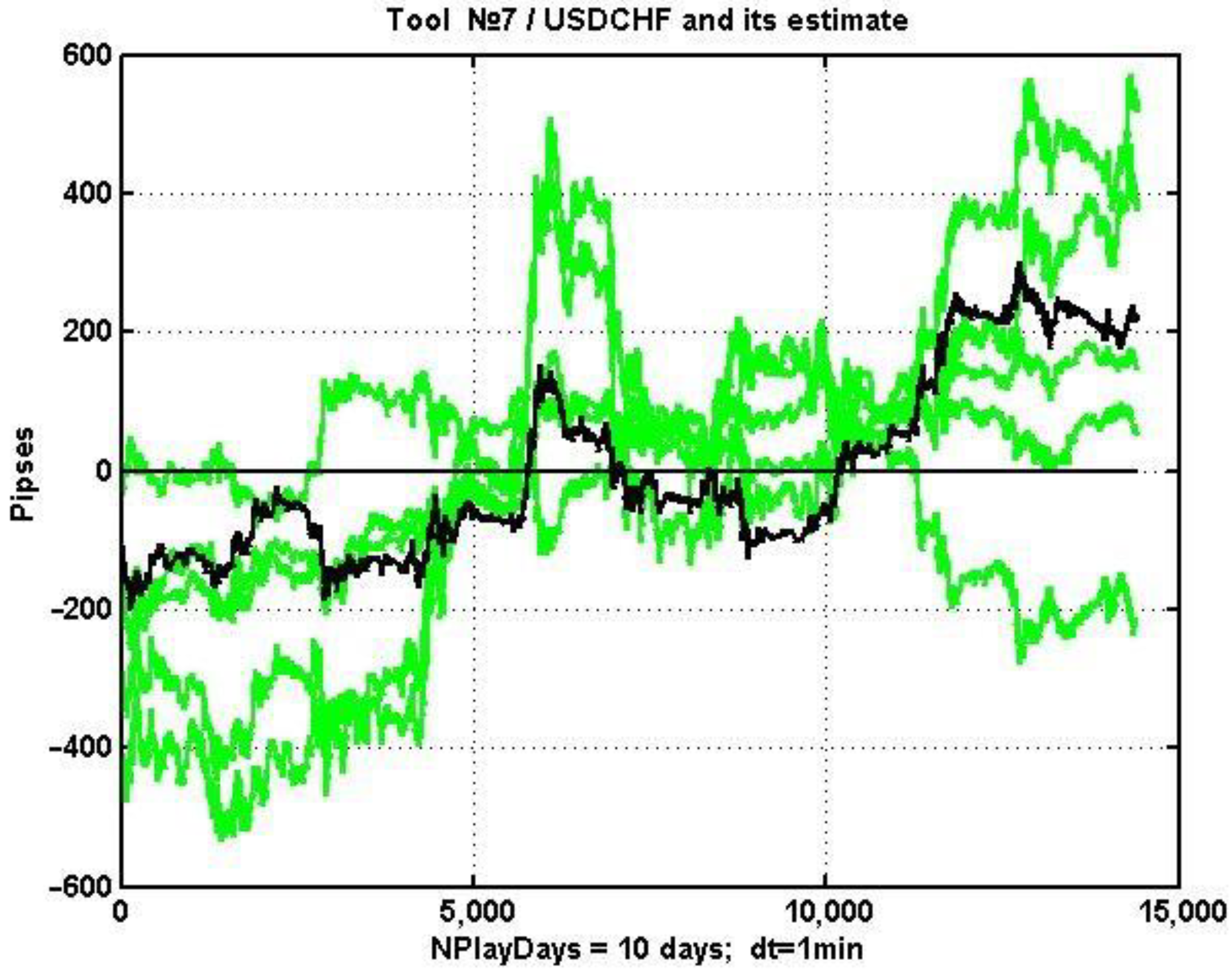
As an example of structural adaptation of the estimation model, consider the problem of choosing a group of regressors for a currency asset that consists of USDCHF.
Figure 10 shows the dynamics of the quotation over ten days against the background of changes in the quotes of the five currency pairs most correlated with it at the specified observation interval. The corresponding group consists of currency pairs with numbers 1, 9, 8, 10, and 16 (see
Table 1).
Note that one of the elements behaves counterphase-like with respect to the considered process. This is due to the degree of the relationship being evaluated by the absolute value. A currency pair with a strong negative correlation also carries a large amount of information about the behavior of the associated instrument. In this case, the corresponding regression coefficient before this term will be negative.
Within the listed constraints, the correlation matrix of the market (i.e., all 16 currency pairs) was recalculated. From the resulting matrix, a row corresponding to the number of the working asset was selected and sorted in descending order of the absolute values of pairwise correlations. The second to (m + 1)th observations of the obtained variation series determine the group of regressors with the largest absolute correlation value. The corresponding results obtained for 24 non-overlapping 10-h observation intervals are presented in
Table 2.
It can be seen that, during the first seven observation intervals, the optimal group of regressors <1 9 8 10 16> did not change. At steps 8–10, the composition of the group was preserved as well, but the first and the ninth regressors swapped places. Further evolution of the group’s composition is clear from the data given in the table. The general conclusion is that the composition changes quite slowly and the 10-day adaptation interval is acceptable for producing regression estimates with given regressors.
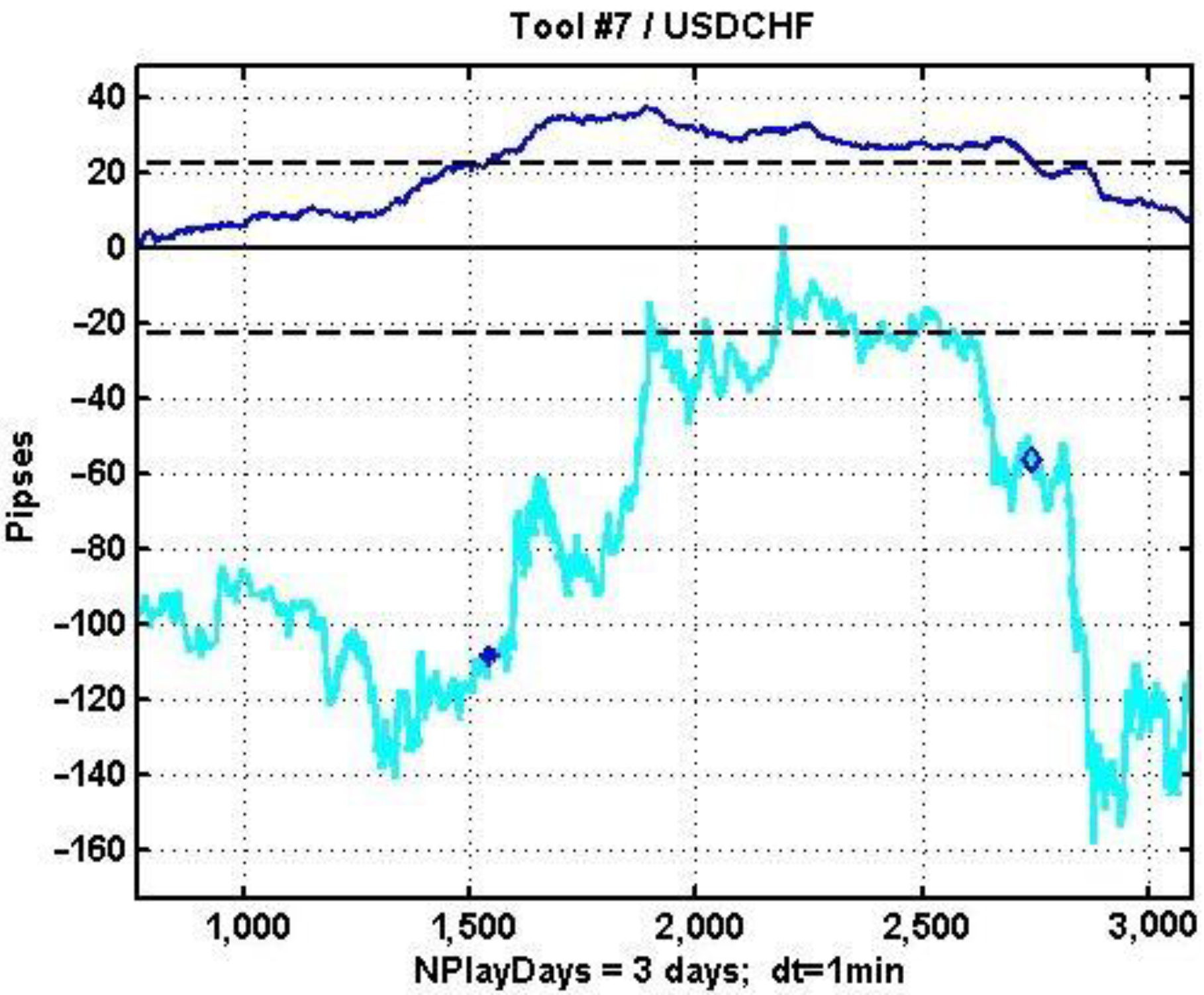
Figure 11 shows a centered plot of the quotation dynamics of the USDCHF currency instrument (bottom) and a smoothed plot of d
k (top) on a three-day observation interval. The same figure shows an example of the implementation of a simple management strategy based on an adaptive MR estimate. If the difference d
k between the estimate and the current value of a currency instrument turns out to be greater (in absolute value) than the threshold value d*, a recommendation is made to open a position in the appropriate direction. The asterisk marks the state of the quote at the time of opening a long position. The diamond corresponds to the position closing at d
k intersecting back the threshold value d*.
The use of structural adaptation in solving the asset management problem with MR estimation increases the frequency of profitable decisions by 5–10%, but does not solve the problem of stability of management in chaotic environments in general.
The reason for this is clear: moving in the oscillator’s direction is determined by its estimate of the prices of financial instruments used as regressors. At the same time, there are external factors that lead to the appearance of dynamic trends. The sum of this movements produces the final form of the dynamics, the direction of which is determined by a vector sum of heterogeneous and hardly forecasted influencing factors.
The absence of an analytical representation of the initial chaotic process does not allow us to obtain an accurate assessment of the potential capabilities of the chosen management strategy. The most effective way to obtain such an estimate is numerical analysis based on random search for optimal parameters of the management strategy. One of the implementations of random search is evolutionary modeling, which has found wide application in numerical optimization problems [
23,
24,
25,
26,
27,
28].
Let us consider the problem of estimating the potential characteristics of the adaptive MR oscillator discussed above based on the evolutionary optimization method. In accordance with the strategy described in the article, a position is opened when the smoothed value dk, k = 1, …, n of the threshold value d* is crossed. The position is closed when the process dk+τ crosses the level d*k+τ back or the zero level dk+τ = 0, where τ is the time of the crossing.
The list of optimized strategy parameters G = [nW, α, d*] (in terms of evolutionary modeling, genome G) includes the size of the sliding observation window nW, which is used to produce a regression estimate, an exponential smoothing coefficient α, and the decision level d*.
At the initial stage, by introducing small (within the limits of the corresponding parameters) variations in all parameters, a group of ancestral genomes (AG) of size Na is formed. Further, in a loop over the number of generations Ng, a new generation is created, consisting of an already existing group of ancestral genomes and a newly generated group of descendant genomes (DG). Descendant genomes are constructed from ancestral genomes in three main ways, including:
Small single changes made to one of the AG parameters. The parameter in question is selected by a random draw. If changes are to be made sequentially to each parameter, then each AG receives mg modifications, where mg is the size of the genome. In this case, there are N(1)d = Namg descendants with a given type of modification, and only one parameter (gene) is modified in each of them. In this case, mg = 3; therefore, if Na = 4 best variants (ancestors) are preserved in each generation, N(1)d = 12 versions of the first type of DG will be obtained.
Small group changes. They are carried out similarly to the previous case, but are made to all parameters at once instead. Thus, there are N(2)d = 4 more versions of DGs with slow changes in all genes.
Strong single mutation or parametric mutation. The AG and the gene number are selected via a random draw. With the probability of parametric mutation, produces N(3)d descendants, in each of which one gene in the range |∆| > 3σ is modified.
As an example, we used a program with Ngc = 9 generation changes in the same time interval of 10 days. As a starting genome, we used a vector G0 = [nW0, α0, d*0] = [5, 0.01, 0.6]. During genome modification, we used rough estimates of the SD of the three listed parameters: SD(G) = [3, 0.02, 0.5].
To compare the potential effectiveness of management strategies based on the MR assessment of the condition of the used asset, we considered two options:
A fixed group of five regressors is selected before the start of trading operations maximizing the correlation with the working instrument (asset). The correlation matrix for all 16 financial instruments is evaluated based on observations of their quotes during the 15 days preceding the start of trading.
Sequential adjustment of a group of five regressors. The adjustment is carried out based on the maximum correlation with the working instrument (asset) with an interval of 10 h. The correlation matrix is evaluated based on the results of observations of their quotes on a sliding observation window of 15 days.
Since the evaluation of gain was carried out via random search, we can only talk about some approximation of the optimal solution, which theoretically could be obtained via brute-force search in the values of the management strategy parameters.
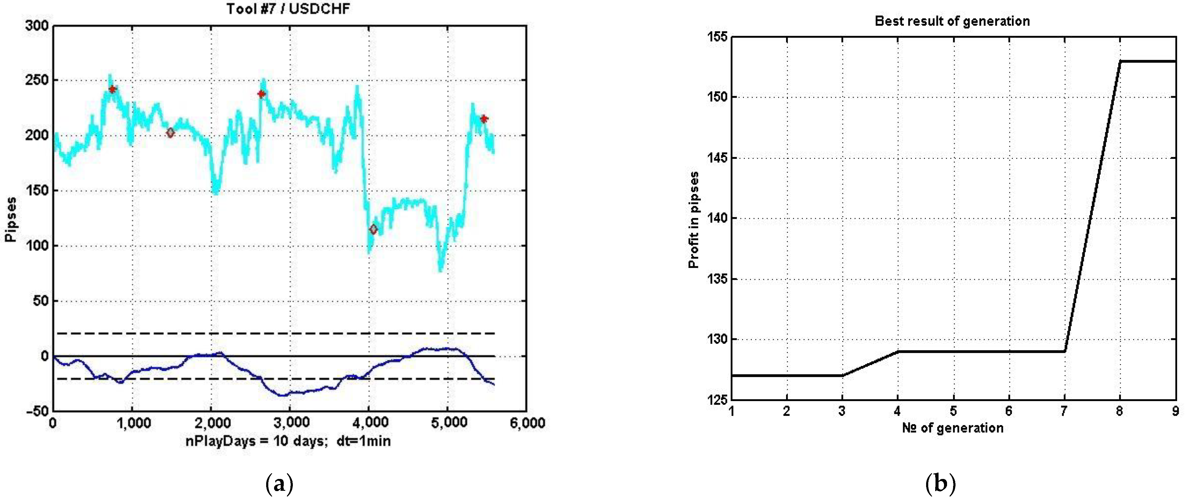
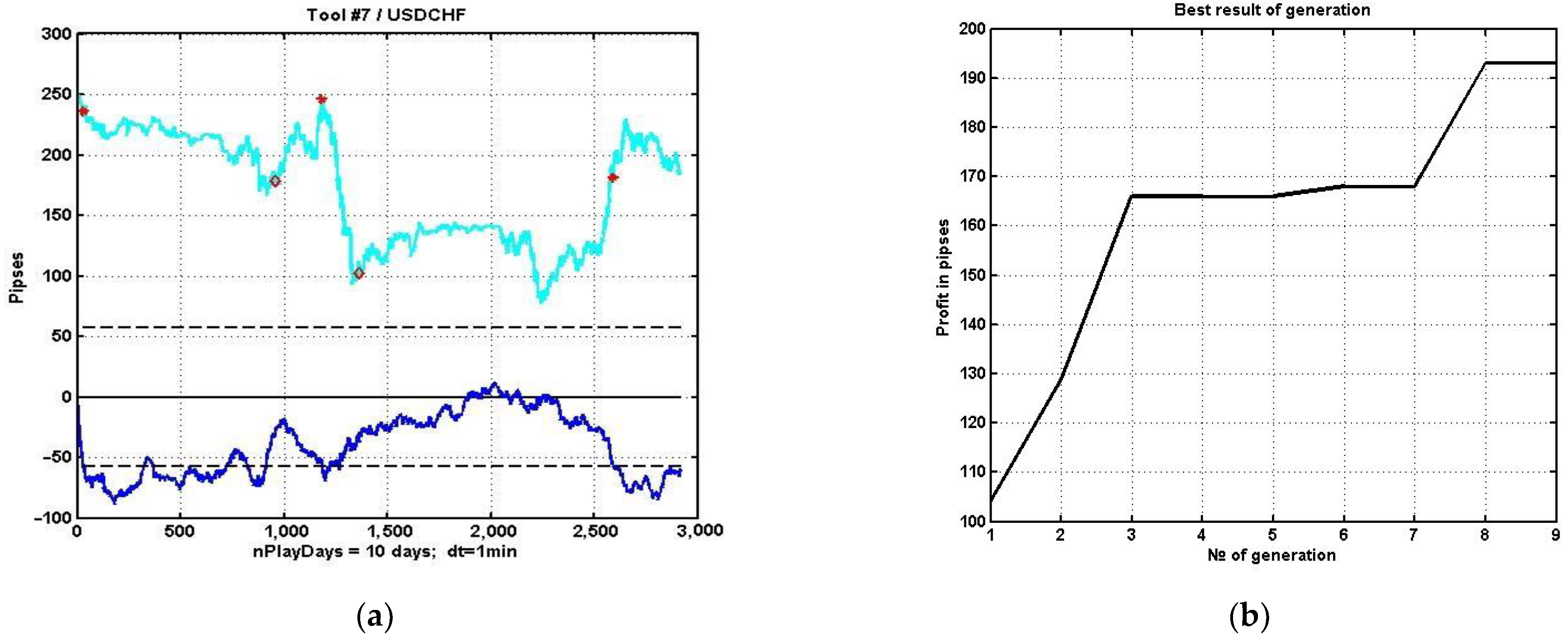
Figure 12a shows an example of the implementation of the best variant of management strategy parameters obtained via evolutionary parametric optimization over nine generations of the corresponding programs. The description of the plots is similar to the description of the processes in
Figure 11. This plot corresponds to the first option, i.e., non-adaptive with respect to the choice of the regressor set.
Figure 12b shows the dependence of the gain growth on the generation number for the non-adaptive strategy.
Similar plots of the implementation of a suboptimal strategy and the dependence of the gain on the generation number for the second option are shown, respectively, in
Figure 13a,b. A comparison of the two examples shows that adaptation during the choice of a group of regressors improves the quality of the estimate and, as a result, increases the potential gain by about 10–15%. Of course, a single example does not give an objective picture of the gain. To generalize the result, we averaged one hundred 10-day observation segments of quotations. Note that averaging over implementations in this case is not equivalent to averaging over one segment of a length equal to the sum of individual implementations. This is due to the fact that the process of price dynamics is not ergodic. Therefore, the task was reproduced for both averaging schemes and, ultimately, showed that the gain from adaptation varies in a wide range of 5% to 15%.
4. Discussion
The research presented in this article is focused on establishing the fundamental possibility of effective proactive management in multidimensional non-stationary, non-linear, and/or chaotic environments. As a basic hypothesis, the assumption is put forward that the market seeks to eliminate the mismatch between the current value of a financial instrument and its valuation, formed by the “opinion” of the market about its “fair price”. The traditional MR evaluation of the instrument was used as such a price in the conducted studies.
In general, the provided numerical studies confirm the hypothesis stated above, but its implementation for an effective management strategy encountered a number of significant difficulties. In particular, the nature of real market processes leads to a significant decrease in the accuracy of the generated estimates of the market value and, consequently, to a decrease in the effectiveness of the asset management process.
The conventional approach to increasing estimate stability for stochastic processes is based on adapting the estimation model to variations in the statistical structure of observation series. However, the effectiveness of adaptation in the tasks of constructing management strategies for chaotic dynamics can be ambiguous. This is due to the fact that real processes, due to their non-stationarity and non-ergodicity, do not allow us to close the adaptation circuit fast enough to have time to track changes in the structure of the observed dynamic process. Therefore, we propose to use the correlation structure of the initial data as a regularizing factor based on processes with relatively slow changes. In particular, as shown in this paper, the adaptation of the estimating model to variations in the correlation structure of multidimensional quotation dynamics can improve the quality of asset value recovery, and, as a result, raise the level of the potential efficiency of the MR oscillator.
5. Conclusions
Selecting a single working component and obtaining its current adjustment based on auxiliary components are problems that arise naturally during the analysis of multidimensional time series that estimate the current values of an indicator from different points of view using different sources of information. In a number of formulations, it turns out that the system of correlations between components has a known inertia, which allows it to be used with some time lag to adjust the current values of the working component. One such formulation of the problem of estimating the current value of a financial instrument is considered in this paper.
Further improvement of estimation quality involves the use of self-organizing algorithms of data analysis and management. In this paper, we investigated the construction of such algorithms using evolutionary modeling, in which the best versions of the observation model are formed by random changes in both the model’s structure and its parameters, with further selection of the most effective solutions in the process of changing generations of models.
The use of self-organization in the task of MR data analysis made it possible to obtain a fundamental confirmation of the viability of the proposed asset management method. However, a stable result with permanent profit was not achieved. This is due to the choice of regressors used for estimating the instrument value being limited to currency pairs available at the electronic Forex exchange. However, other parameters may have a greater influence on a particular financial instrument in a given time interval. These parameters could describe dynamic processes in the stock or commodity market or in the market infrastructure associated with political, military, environmental, and other factors.
Another direction of development of this approach is based on the robustification of estimation algorithms [
29,
30], i.e., reducing the sensitivity of estimates to variations in the statistical structure of the data. In principle, this approach could serve as an alternative to adaptation technologies that are insufficiently effective due to the inertia-free and chaotic nature of the initial series of observations. However, the price of increased stability is a decrease in accuracy. Thus, this issue requires separate research.


