
Quadratic B-Spline Surfaces with Free Parameters for the Interpolation of Curve Networks


Abstract
:1. Introduction
2. The Network of B-Spline Curves
- C1.
- all the curves are defined onand all the curves are defined on
- C2.
- there exist parametersandsuch that
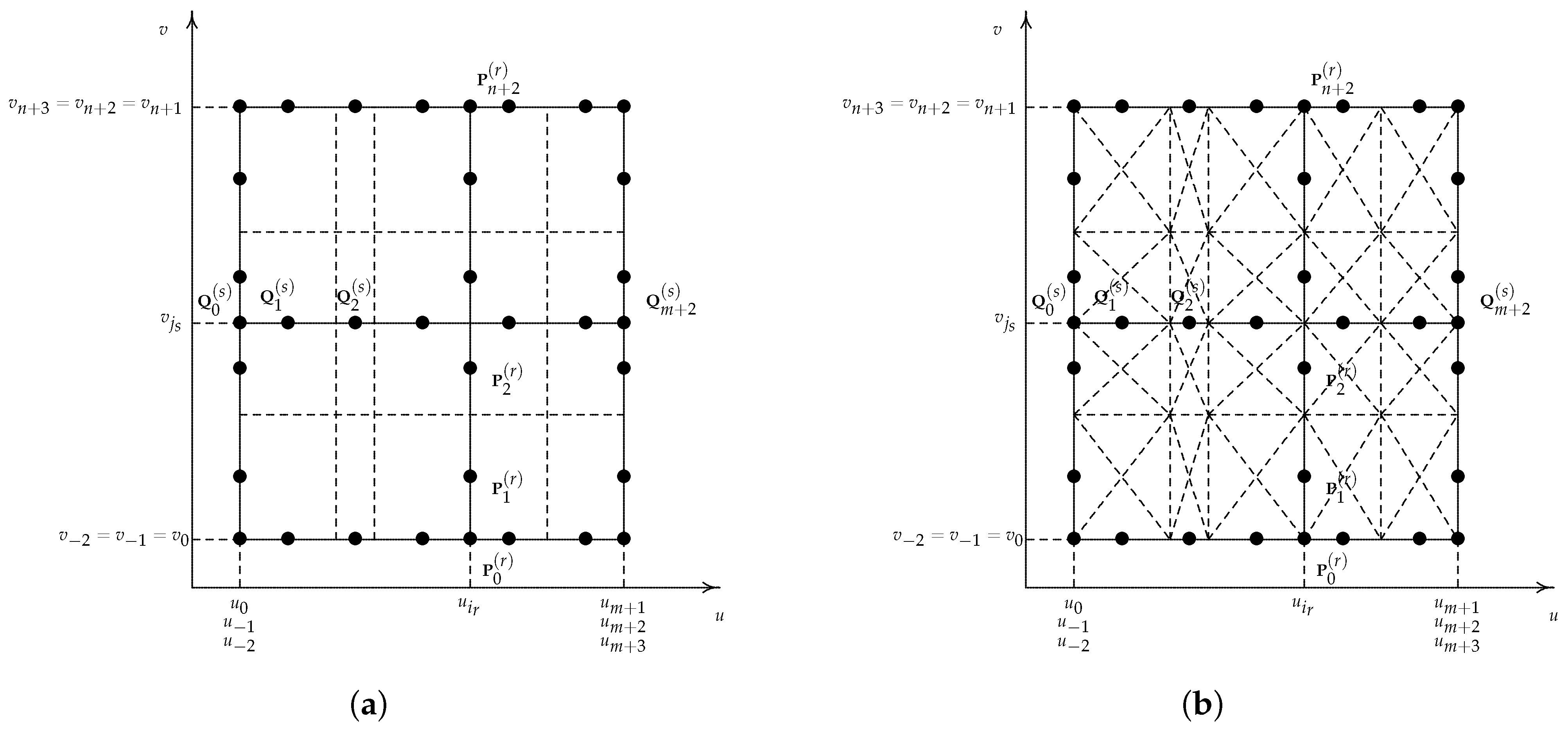
3. Construction of the Interpolating B-Spline Surface
- -
- the knots in the partitions U and V not associated to a curve of the network are barriers identifying subdomains in . In each subdomain, we have a minimal configuration;
- -
- the number of subdomains in is equal to ;
- -
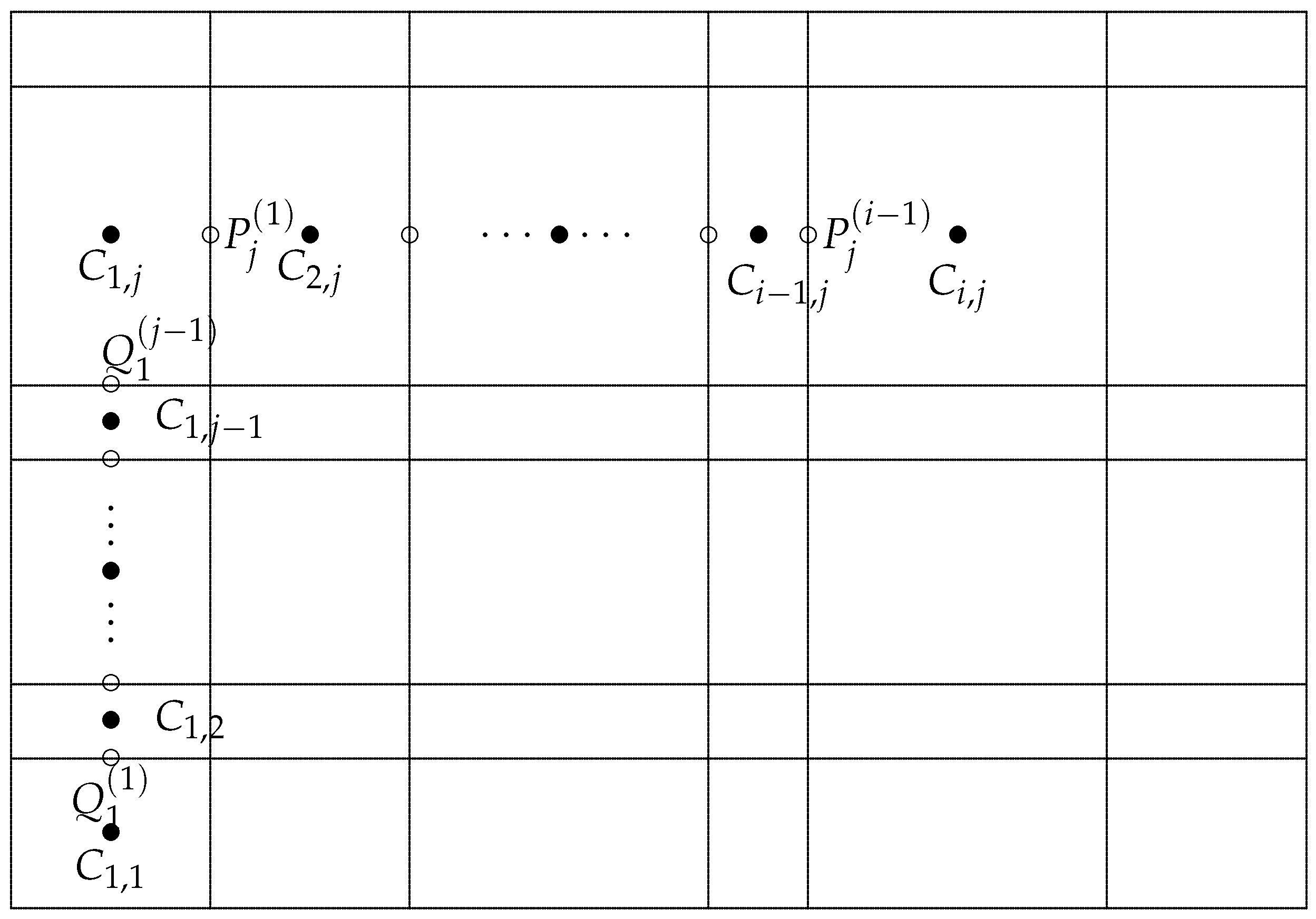
- the control point in the left-down corner of each subdomain is identified as a free parameter;
- -
- the control point is always a free parameter.
- -
- is the index of the last barrier before the control point in the direction U, i.e., ;
- -
- is the index of the last barrier before the control point in the direction V, i.e., ;
- -
- α is the number of barriers in the direction U before the control point ;
- -
- β is the number of barriers in the direction V before the control point .
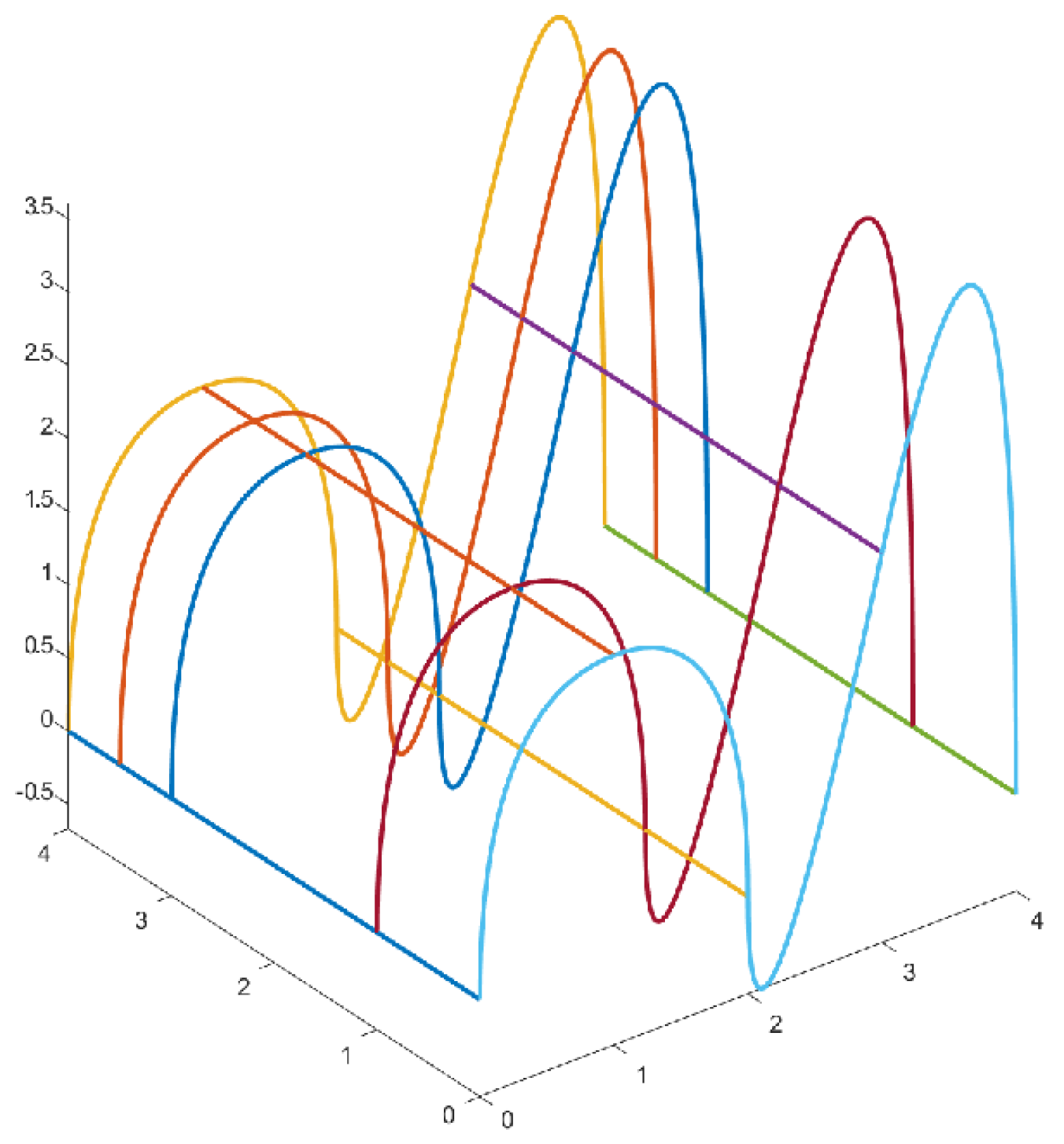
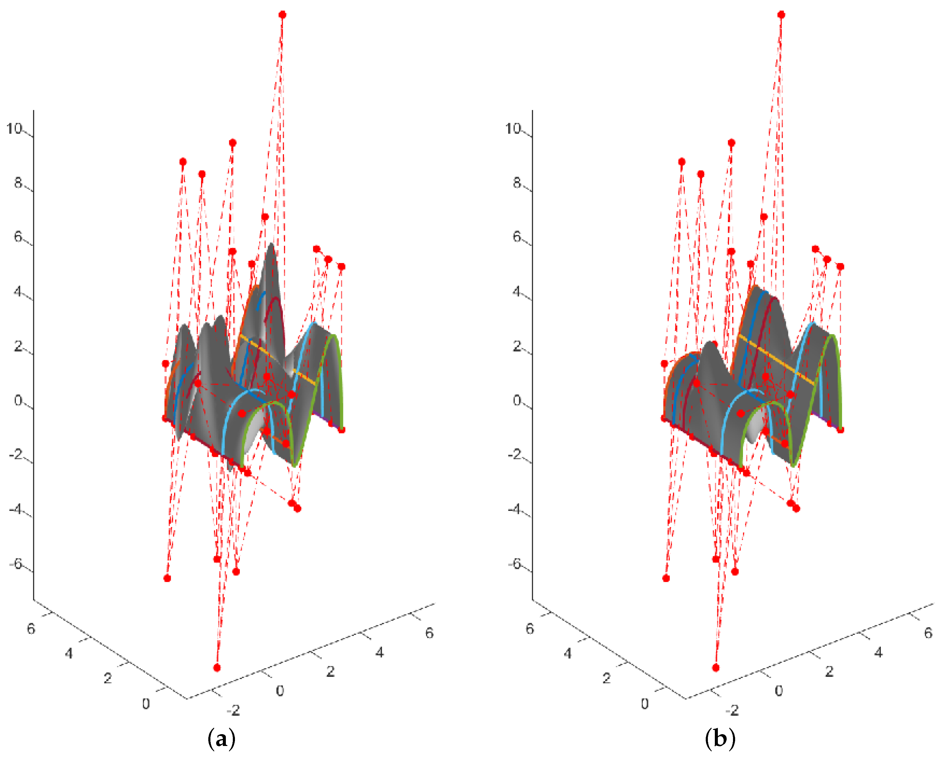
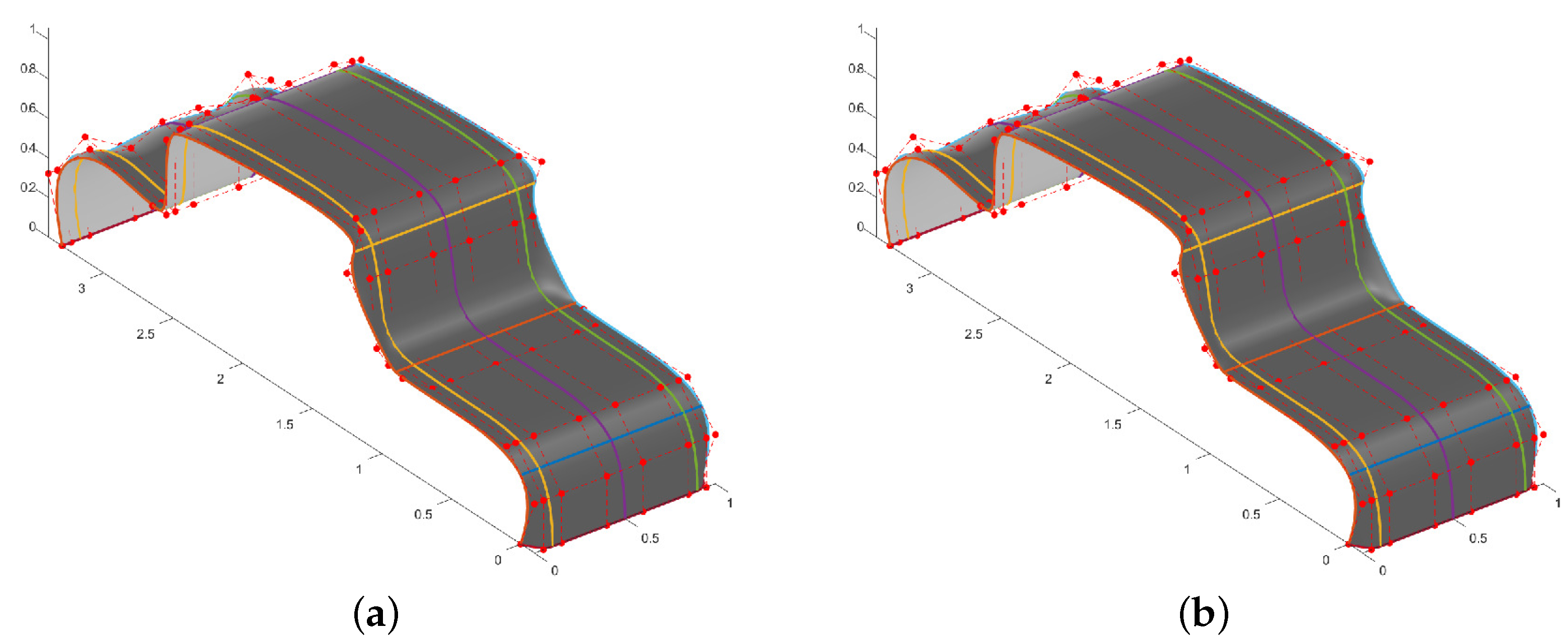
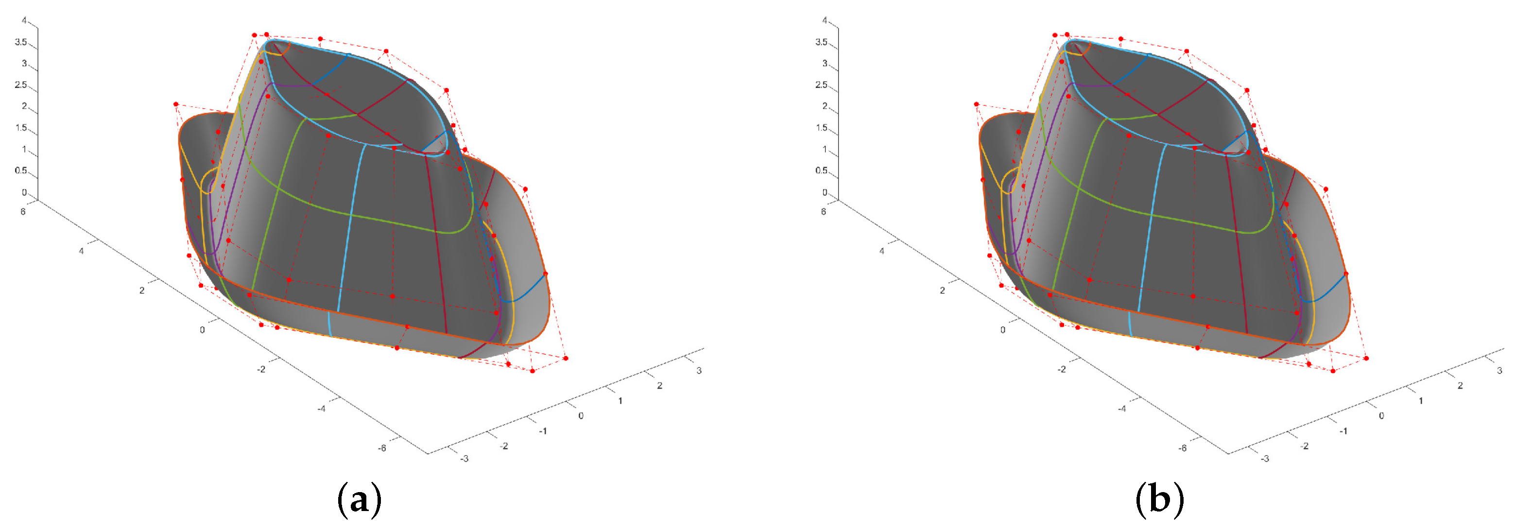
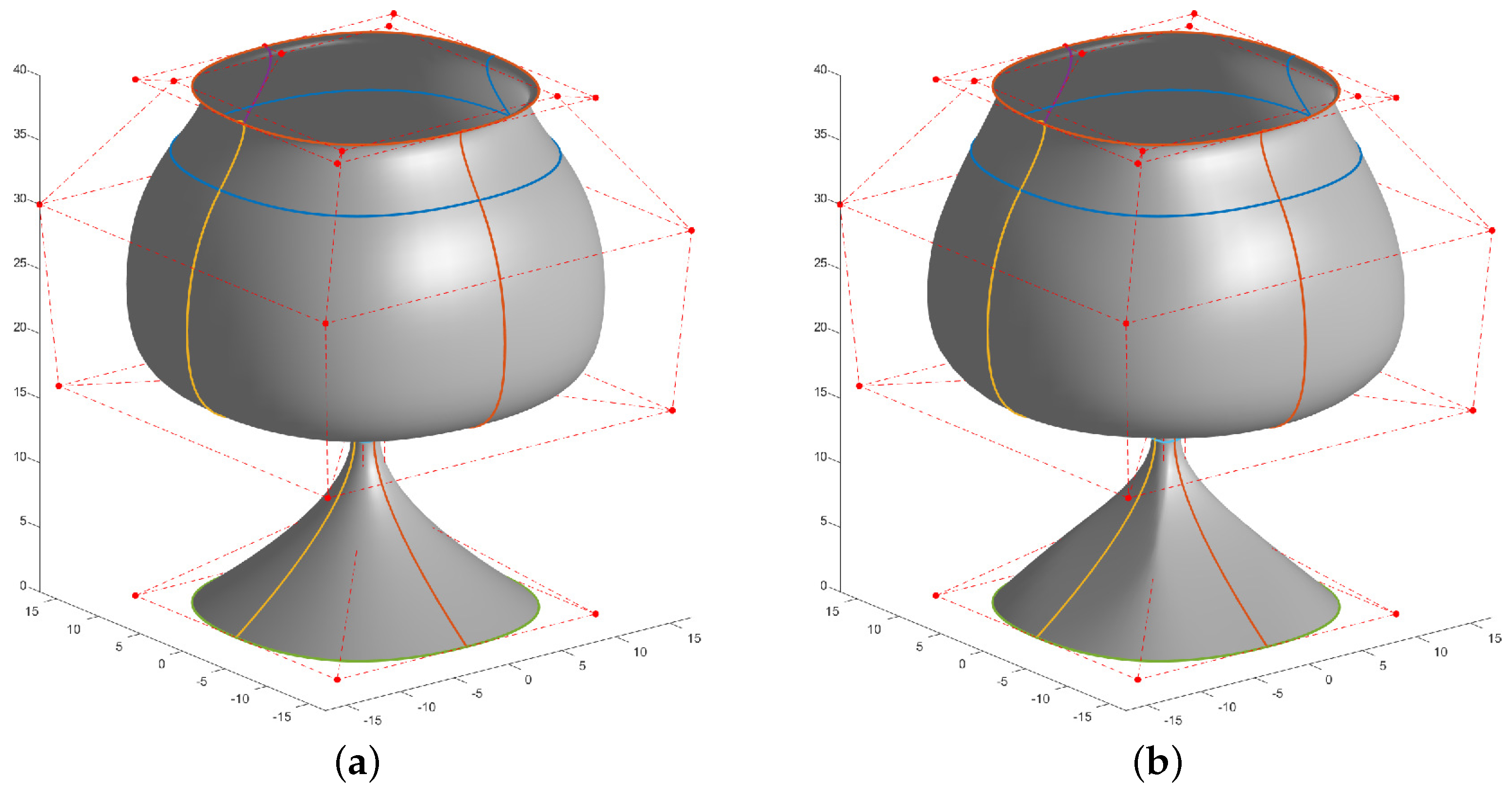
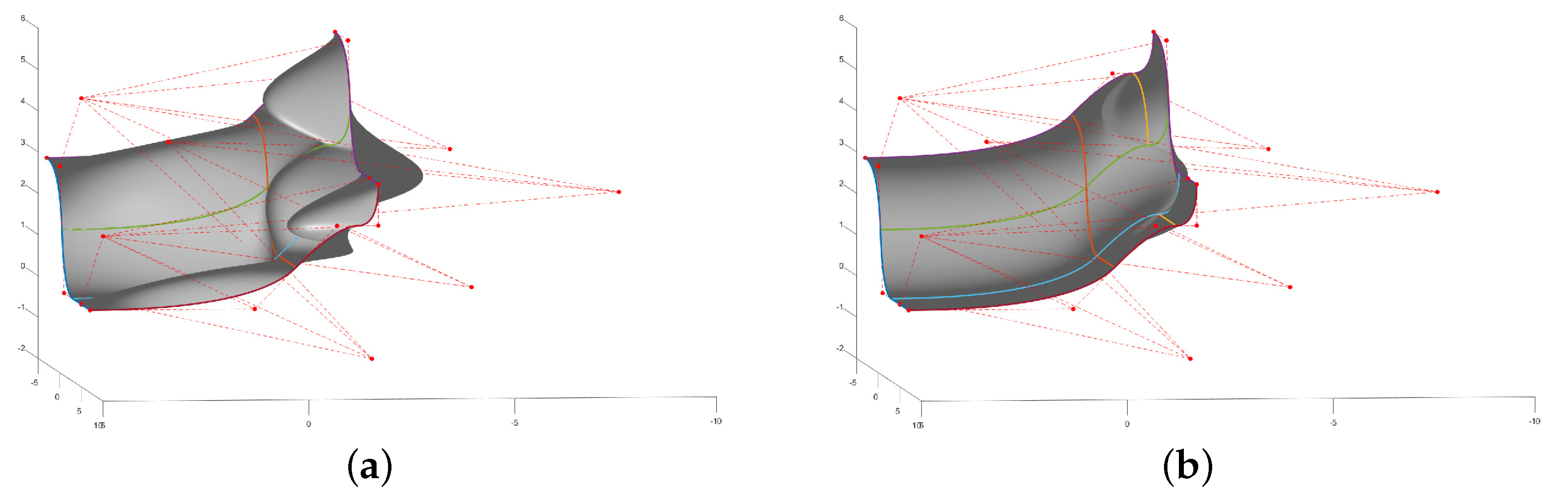
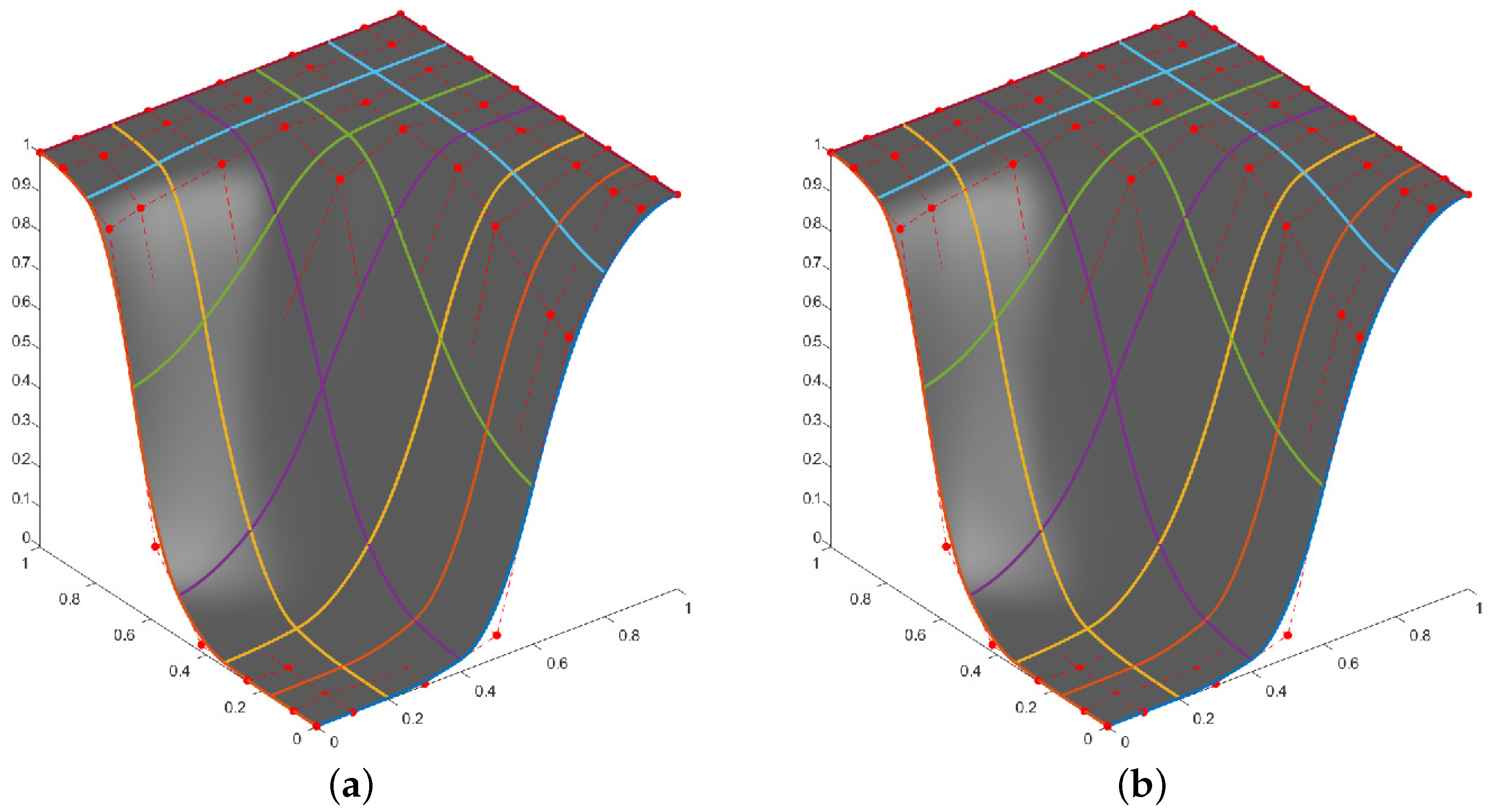
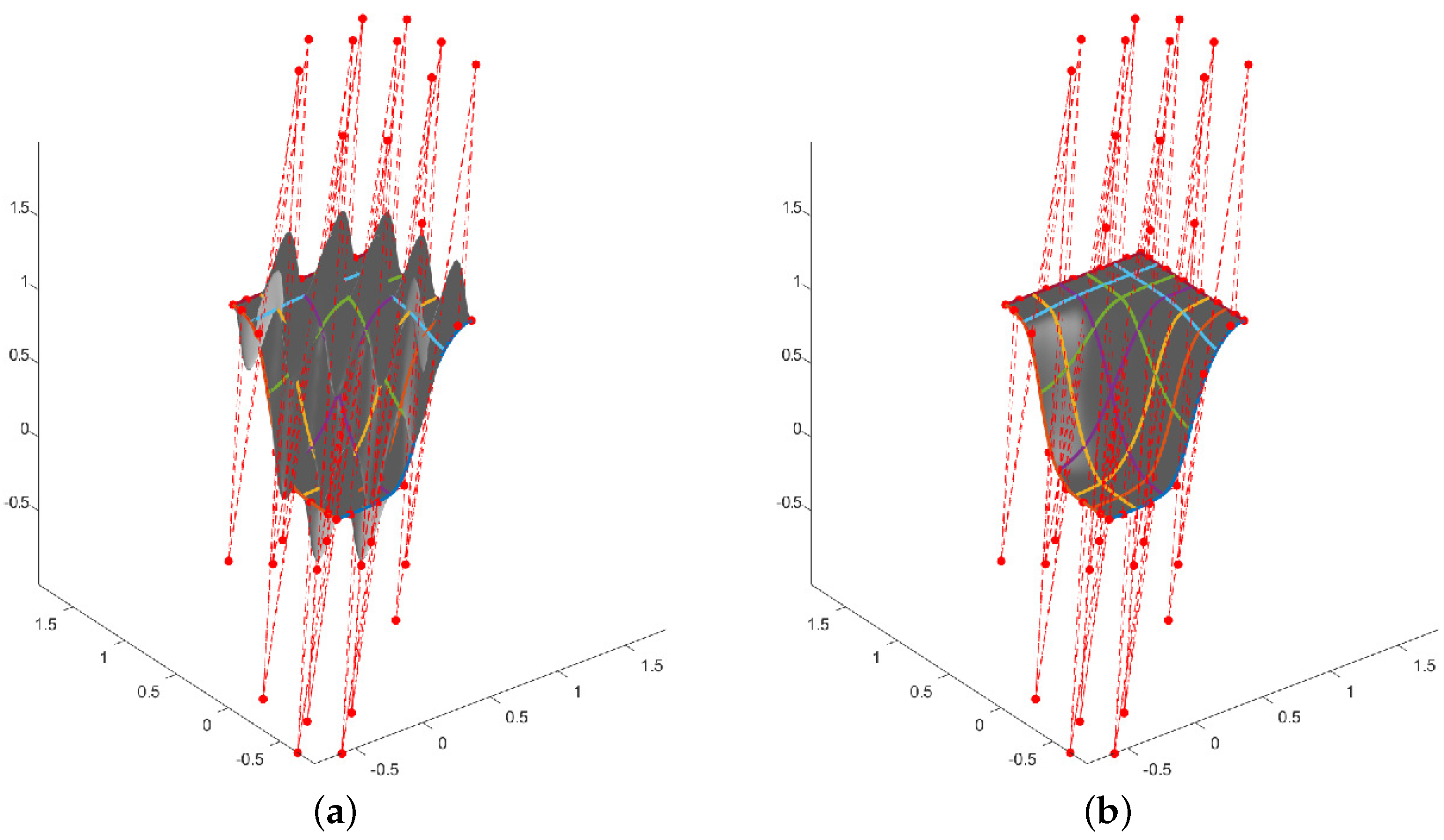
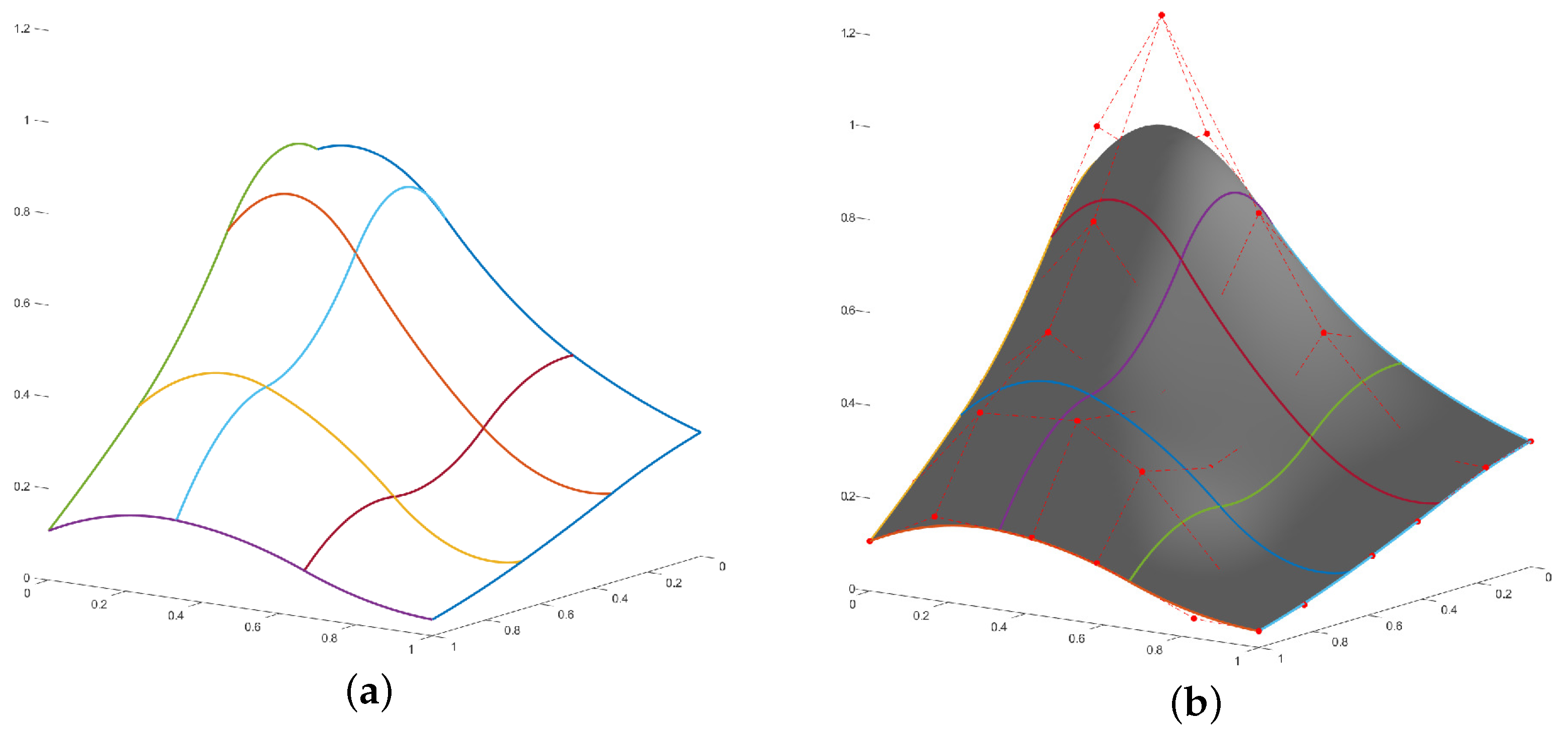
4. Numerical Results
4.1. Test 1
4.2. Test 2
4.3. Test 3
4.4. Test 4
4.5. Test 5
5. Conclusions
Author Contributions
Funding
Institutional Review Board Statement
Informed Consent Statement
Data Availability Statement
Acknowledgments
Conflicts of Interest
References
- Barnhill, R.E. Blending function interpolation: A survey and some new results. In Numerische Methoden der Approximationstheorie; Collatz, L., Werner, H., Meinardus, G., Eds.; Birkhauser Verlag: Basel, Switzerland, 1976; Volume 3, pp. 43–89. [Google Scholar]
- Bos, L.P.; Grabenstetter, J.E.; Salkauskas, K. Pseudo-tensor product interpolation and blending with families of univariate schemes. Comput. Aided Geom. Des. 1996, 13, 429–440. [Google Scholar] [CrossRef]
- Delvos, J.; Schempp, W. Boolean Methods in Interpolation and Approximation; Longman Scientific and Technical: Harlow, UK, 1989. [Google Scholar]
- Gordon, W.J. Spline blended interpolation through curve networks. J. Math. Mech. 1969, 18, 931–952. [Google Scholar]
- Gordon, W.J. Blending-function methods of bivariate and multivariate interpolation. SIAM Numer. Anal. 1971, 8, 158–177. [Google Scholar] [CrossRef]
- Gordon, W.J. Sculptured surface definition via blending function methods. In Fundamental developments of Computer Aided Geometric Modeling; Piegl, L., Ed.; Academic Press: London, UK, 1993. [Google Scholar]
- Peters, J. Smooth interpolation of a mesh of curves. Constr. Approx. 1991, 7, 221–246. [Google Scholar] [CrossRef]
- Conti, C.; Dyn, N. Blending based Chaikin type subdivision schemes for nets of curves. In Mathematical Methods for Curves and Surfaces; Daehlen, M., Morken, K., Schumaker, L.L., Eds.; Nashboro Press: Brentwood, TN, USA, 2005; pp. 51–68. [Google Scholar]
- Greshake, S.H.; Bronsart, R. Application of subdivision surfaces in ship hull form modeling. Comput.-Aided Des. 2018, 100, 79–92. [Google Scholar] [CrossRef]
- Piegl, L.; Tiller, W. The NURBS Book; Springer: Berlin/Heidelberg, Germany, 1995. [Google Scholar]
- Bouhiri, S.; Lamnii, A.; Lamnii, M.; Zidna, A. A C1 composite spline Hermite interpolant on the sphere. Math. Meth. Appl. Sci 2021, 44, 11376–11391. [Google Scholar] [CrossRef]
- Wang, R.H.; Li, C.J. A kind of multivariate NURBS surfaces. J. Comput. Appl. Math. 2004, 22, 137–144. [Google Scholar]
- Wang, R.H.; Li, C.J. Bivariate cubic spline space and bivariate cubic NURBS surfaces. In Proceedings of the Geometric Modeling and Processing 2004, Beijing, China, 13–15 April 2004; pp. 115–123. [Google Scholar]
- Wang, R.H.; Li, C.J. The multivariate quartic NURBS surfaces. J. Comput. Appl. Math. 2004, 163, 155–164. [Google Scholar]
- Dagnino, C.; Lamberti, P.; Remogna, S. Curve network interpolation by C1 quadratic B-spline surfaces. Comput. Aided Geom. Des. 2015, 40, 26–39. [Google Scholar] [CrossRef] [Green Version]
- Sablonnière, P. On some multivariate quadratic spline quasi-interpolants on bounded domains. In Modern Developments in Multivariate Approximations; Hausmann, W., Ed.; Birkhäuser Verlag: Basel, Switzerland, 2003; Volume 145, pp. 263–278. [Google Scholar]
- Sablonnière, P. Quadratic spline quasi-interpolants on bounded domains of , d = 1, 2, 3. Rend. Sem. Mat. Univ. Pol. Torino 2003, 61, 229–246. [Google Scholar]
- de Boor, C. A Practical Guide to Splines; Revised edition; Springer: Berlin, Germany, 2001. [Google Scholar]
- Chui, C.K. Multivariate Splines; CBMS-NSF Regional Conference Series in Applied Mathematics; SIAM: Philadelphia, PA, USA, 1988; Volume 54. [Google Scholar]
- Chui, C.K.; Wang, R.H. Concerning C1 B-splines on triangulations of non-uniform rectangular partition. Approx. Theory Appl. 1984, 1, 11–18. [Google Scholar]
- Dagnino, C.; Lamberti, P. On the construction of local quadratic spline quasi-interpolants on bounded rectangular domains. J. Comput. Appl. Math. 2008, 221, 367–375. [Google Scholar] [CrossRef] [Green Version]
- Wang, R.H. Multivariate Spline Functions and Their Applications; Science Press: Beijing, China; New York, NY, USA; Kluwer Academic Publishers: Dordrecht, The Netherlands; Boston, MA, USA; London, UK, 2001. [Google Scholar]
- Dagnino, C.; Lamberti, P.; Remogna, S. BB-Coefficients of Unequally Smooth Quadratic B-Splines on Non Uniform Criss-Cross Triangulations. Quaderni Scientifici del Dipartimento di Matematica, Università di Torino, 2008 n. 24. Available online: http://hdl.handle.net/2318/434 (accessed on 4 February 2022).
- Dagnino, C.; Lamberti, P.; Remogna, S. B-spline bases for unequally smooth quadratic spline spaces on non-uniform criss-cross triangulations. Numer. Algorithms 2012, 61, 209–222. [Google Scholar] [CrossRef] [Green Version]
- Wang, R.H.; He, T. The spline spaces with boundary conditions on nonuniform type-2 triangulation. Kexue Tongbao 1985, 30, 858–861. [Google Scholar]
- Conti, C.; Sestini, A. Choosing nodes in parametric blending function interpolation. Comput. Aided Des. 1996, 28, 135–143. [Google Scholar] [CrossRef]
- Hadenfeld, J. Local energy fairing of B-spline surfaces. In Mathematical Methods for Curves and Surfaces: Ulvik, 1994; Daehlen, M., Lyche, T., Schumaker, L.L., Eds.; Vanderbilt Univ. Press: Nashville, TN, USA, 1995; pp. 203–212. [Google Scholar]
- Lyness, J.N.; Cools, R. A survey of numerical cubature over triangles. Proc. Symp. Appl. Math. 1994, 48, 127–150. [Google Scholar]
- von Winckel, G. Matlab Procedure Triquad. Available online: http://www.mathworks.com/matlabcentral/fileexchange/9230-gaussian-quadrature-for-triangles (accessed on 4 February 2022).


Publisher’s Note: MDPI stays neutral with regard to jurisdictional claims in published maps and institutional affiliations. |
© 2022 by the authors. Licensee MDPI, Basel, Switzerland. This article is an open access article distributed under the terms and conditions of the Creative Commons Attribution (CC BY) license (https://creativecommons.org/licenses/by/4.0/).
Share and Cite
Lamberti, P.; Remogna, S. Quadratic B-Spline Surfaces with Free Parameters for the Interpolation of Curve Networks. Mathematics 2022, 10, 543. https://doi.org/10.3390/math10040543
Lamberti P, Remogna S. Quadratic B-Spline Surfaces with Free Parameters for the Interpolation of Curve Networks. Mathematics. 2022; 10(4):543. https://doi.org/10.3390/math10040543
Chicago/Turabian StyleLamberti, Paola, and Sara Remogna. 2022. "Quadratic B-Spline Surfaces with Free Parameters for the Interpolation of Curve Networks" Mathematics 10, no. 4: 543. https://doi.org/10.3390/math10040543
APA StyleLamberti, P., & Remogna, S. (2022). Quadratic B-Spline Surfaces with Free Parameters for the Interpolation of Curve Networks. Mathematics, 10(4), 543. https://doi.org/10.3390/math10040543