Adaptive Guided Spatial Compressive Cuckoo Search for Optimization Problems

Abstract

Cuckoo Search (CS) is one of the heuristic algorithms that has gradually drawn public attention because of its simple parameters and easily understood principle. However, it still has some disadvantages, such as its insufficient accuracy and slow convergence speed. In this paper, an Adaptive Guided Spatial Compressive CS (AGSCCS) has been proposed to handle the weaknesses of CS. Firstly, we adopt a chaotic mapping method to generate the initial population in order to make it more uniform. Secondly, a scheme for updating the personalized adaptive guided local location areas has been proposed to enhance the local search exploitation and convergence speed. It uses the parent’s optimal and worst group solutions to guide the next iteration. Finally, a novel spatial compression (SC) method is applied to the algorithm to accelerate the speed of iteration. It compresses the convergence space at an appropriate time, which is aimed at improving the shrinkage speed of the algorithm. AGSCCS has been examined on a suite from CEC2014 and compared with the traditional CS, as well as its four latest variants. Then the parameter identification and optimization of the photovoltaic (PV) model are applied to examine the capacity of AGSCCS. This is conducted to verify the effectiveness of AGSCCS for industrial problem application.

1. Introduction

The optimization problems cover a wide range, including economic dispatch [1], data clustering [2], structure design [3], image processing [4], and so on. The aim of optimization is to find the optimal solution only when the constraint conditions are satisfied. If the optimization has no constraint conditions, it is named an unconstrained optimization. Otherwise, it is called a constraint optimization problem [5]. A mathematical model is derived below, which can be concluded in most of the above cases:

$$\left\{\begin{array}{c}minimize:\hspace{1em}\hspace{1em}f\left(x\right)\\ subject to:\hspace{1em}g\left(x\right)\le 0, h\left(x\right)=0\\ g\left(x\right)=\{g_1\left(x\right),g_2\left(x\right),\dots ,g_m\left(x\right)\\ h\left(x\right)=\left\{h_1\left(x\right),h_2\left(x\right),\dots ,h_n\left(x\right)\right\}\end{array}\right.$$

(1)

where f(x) is the objective function, $i$ exhibits the number of objective functions, g(x) and h(x) are constraint functions, g(x) is an inequality constraint and h(x) is an equality constraint. When the problem is unconstrained, g(x) and h(x) are equal to 0 and m and n represent the number of constraints, respectively.

To solve the optimization problem, various solutions have been proposed. In the beginning, some accurate numerical algorithms were developed, such as gradient descent technology [6,7], linear programming [8], nonlinear programming [9], quadratic programming [10,11], Lagrange multiplier method [12,13] and λ-iteration method [14,15]. However, these numerical methods do not show absolute computational advantages in high-dimensional problems. Contrarily, it loses time because of its accurate search methods [16]. Later on, some heuristic algorithms are gradually invented. The earliest and most famous one is the genetic algorithm (GA), first proposed in the 1970s by John Holland [17]. It draws lessons from the process of chromosome gene crossover and mutation in biological evolution to transform the accurate solution of the problem into an optimization. Since heuristic algorithms often lack global guidance rules, they are easy to fall into local stagnation. In the past two decades, some intelligent algorithms imitating the biological behavior of nature have begun to appear, which are called metaheuristics. Particle Swarm Optimization (PSO) can be regarded as one of the earliest swarm intelligence algorithms [18]. PSO is a random search algorithm based on group cooperation, which simulates the foraging behavior of birds. A bat-inspired algorithm (BA) was proposed by X.S. Yang et al. [19]. The BA makes use of the process of a bat population moving and searching prey. The Artificial Bee Colony Algorithm (ABC) was invented by Karaboga et al. [20]. It is a metaheuristic algorithm that imitates bee foraging behavior. It regards the population as bees and divides bees into several species. Different bees exchange information in a specific way, thereby guiding the bee colony to a better solution. The Grey Wolf Optimizer (GWO) is another metaheuristic algorithm and was proposed by Mirjalili [21]. It has three intelligent behaviors containing encircling prey, hunting, and attacking. In addition, the Cuckoo Search (CS) algorithm was proposed by Xin-She Yang [22]. CS is a nature-inspired algorithm that imitates the brood reproductive strategy of cuckoo birds to increase the survival probability of their offspring. Different from other metaheuristic algorithms, CS adapts its parameters by relying on the random walk possibility $P_a$, which is easy to control for the iterations of the simple parameters. What is more, CS adopts two searching methods including $L\mathit{é}vy$ Flight and random walk flight. This combination of large and small step size makes the global searchability stronger when compared with other algorithms.

Although CS has been easily accepted, there are still some weaknesses, such as insensitive parameters and easy convergence to the local optimal [23,24]. Commonly, conventional improvements for CS mainly aim at the following steps:

(1)

Improve $L\mathit{é}vy$ Flight. $L\mathit{é}vy$ Flight is proposed to enhance the disorder and randomness in the search process to increase the diversity of solutions. It combines considerable step length with a small step length to strengthen global searchability. Researchers modified $L\mathit{é}vy$ Flight to achieve a faster convergence. Naik cancelled the step of $L\mathit{é}vy$ flight and made the adaptive step according to the fitness function value and its current position in the search space [25]. In reference [26], Ammar Mansoor Kamoona improved CS by replacing the Gaussian random walk with a virus diffusion instead of the Lévy flights for a more stable process of nest updating in traditional optimization problems. Hu Peng et al. [27] used the combination of Gaussian distribution and $L\mathit{é}vy$ distribution to control the global search by means of random numbers. S. Walton et al. [28] changed the step size generation method in $L\mathit{é}vy$ flight and obtained a better performance. A new nearest neighbor strategy was adopted to replace the function of $L\mathit{é}vy$ flight [29]. Moreover, he changed the strategy for crossover in global search. Jiatang Cheng et al. [30] drew lessons from ABC and employed two different one-dimensional update rules to balance the global and local search performance.

However, the above work is always aimed at global search. Too much attention is paid to global search and ignores local search. $L\mathit{é}vy$ flight provides a rough position for the optimization process, while local walking deteriorates the mining ability of CS. Therefore, the improvement of local walking is also important.

(2)

Secondly, the parameter and strategy adjustment have always been a significant concern for improving the metaheuristic algorithm. The accuracy and convergence speed of CS are increased through the adaptive adjustment of parameters or the innovation of strategies in the algorithm. For example, Pauline adopted a new adaptive step size adjustment strategy for the $L\mathit{é}vy$ Flight weight factor, which can converge to the global optimal solution faster [31]. Tong et al. [32] proposed an improved CS; ImCS drew on the opposite learning strategy and combined it with the dynamic adjustment of the score probability. It was used for the identification of the photovoltaic model. Wang et al. [33] used chaotic mapping to adjust the step size of cuckoo in the original CS method and applied an elite strategy to retain the best population information. Hojjat Rakhshani et al. [34] proposed two population models and a new learning strategy. The strategy provided an online trade-off between the two models, including local and global searches via two snap and drift modes.

These approaches in this area have indeed improved the diversity of the population. However, in adaptive and multi-strategy methods, the direction of the optimal solution is often used as the reference direction for the generation of children. If the population searches along the direction of the optimal solution, the population may be trapped into a local optimization. In addition, the elite strategy based on a single optimal solution rather than a group solution is not stable enough. Once the elite solution does not take effect, it will affect the iterative process of the whole solution group.

(3)

Thirdly, the combination of optimization and other algorithms is another improvement focus. For example, M. Shehab et al. [35] innovatively adopted the hill-climbing method into CS. The algorithm used CS to obtain the best solution and passed the solution to the hill-climbing algorithm. This intensification process accelerated the search and overcame the slow convergence of the standard CS algorithm. Jinjin Ding et al. [23] combined PSO with CS. The selection scheme of PSO and the elimination mechanism of CS gave the new algorithm a better performance. DE and CS also could be combined. In ref [36], Z. Zhang et al. made use of the characteristics of the two algorithms dividing the population into two subgroups independently.

This kind of improvement method generally uses one algorithm to optimize the parameters of another algorithm. Later, global optimization would be carried out. This method has strong operability, but there are two or more cycles, which increases the complexity of the algorithm.

Based on the above discussion, we proposed three strategies to solve the above problems of CS. Firstly, a scheme of initializing the population by chaotic mapping has been proposed to solve the problem of uneven distribution in high-dimensional cases. Experiments show that the iterative operation using the chaotic sequence as the initial population will influence the whole process of the algorithm [33]. Furthermore, this often achieves better results than a pseudo-random number [37]. Secondly, aiming at enhancing the process of random walk, we put forward an adaptive guided local search method, which reduces the instability of randomness by the original local search. This search method ranks all of the species according to their adaptability. In this segment, we believe that the information for optimal solutions and poor solutions are both important to the iterative process. Thus, the position of the best of the first $p\%$ and the worst of the last $p\%$ calculates the difference and gets the direction of the next generation’s solution. This measure reasonably takes advantage of the best and worst solutions because they are considered to have potential information related to the ideal solution [38]. The solution group ensures the universality of the optimization process and avoids the occurrence of individual abnormal solutions affecting the optimization direction. Thirdly, as discussed before, to increase the optimization ability some researchers like to use different algorithms combined with CS. However, compared with the original CS, this measure increases many additional segments. Moreover, there is added algorithm complexity, which wastes computational time. Therefore, we propose a spatial compression (SC) technique that positively impacts the algorithm from the outside. The SC technique was firstly proposed by A. Hirrsh and can help the algorithm converge by artificial extrusion [39]. This method that adjusts the optimization space with the help of external pressure has been proved to be effective [40].

We incorporated these three improvements into CS and propose an Adaptive Guided Spatial Compressive CS (AGSCCS). It has the following merits compared with CS and other improved algorithms: (1) An even and effective initial population. This population generation method is applicable when solving high-dimensional problems. (2) Reasonable and efficient information from each generation of optimal solutions while avoiding the population search bias caused by random sequences. (3) Increasing the precision of the population iteration while maintaining the convergence rate. The imposed spatial compression also boosts the exploration power of the algorithm to some extent, as it could identify potentially viable regions, judge the next direction of spatial reduction, and avoid getting trapped in local optimal. The AGSCCS algorithm will be simulated and compared on 30 reference functions with single, multi-peak, rotation, and displacement characteristics. Moreover, we also applied the proposed algorithm to the photovoltaic (PV) model problem to verify its feasibility for practical issues. Research on PV systems is vital for the efficient use of renewable energy. Its purpose is to accurately, stably, and quickly identify the important parameters in the PV model. The results show that both the effectiveness and efficiency of the proposed algorithm are proven. Compared with other algorithms, the new algorithm is competitive in dealing with various optimization problems, which is mainly reflected in:

(1)

An initialization method of a logistic chaotic map is used to replace the random number generation method regardless of the dimension.

(2)

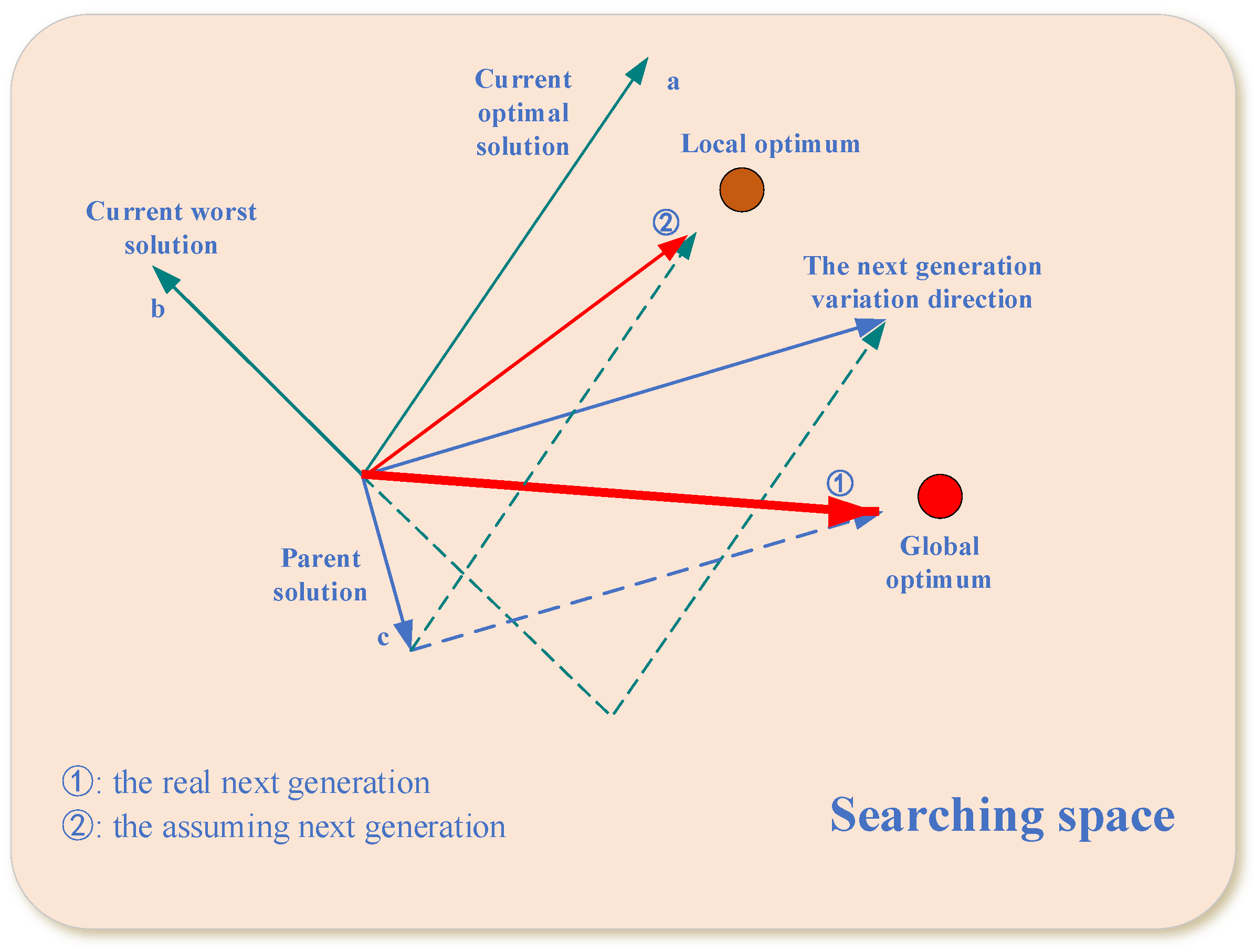
A guiding method that includes the information of optimal solutions and worst solutions is used to facilitate the generation of offspring.

(3)

An adaptive update step size replaces the random step size to make the search radius more reasonable.

(4)

In the iterative process, the SC technique is added to compress the space to help rapid convergence artificially.

The rest of the thesis is divided into the following six parts. The introduction of the original CS is briefly exhibited in Section 2. Section 3 concisely introduces the main idea of AGSCS. In Section 4, the experimental simulation results and their interpretations are presented. Furthermore, a sensitive discussion is performed to compare the enhancement of the improved strategies. In Section 5, AGSCCS is applied to the parameter identification and optimization of the PV model. The work is summarized in Section 6.

2. Cuckoo Search (CS)

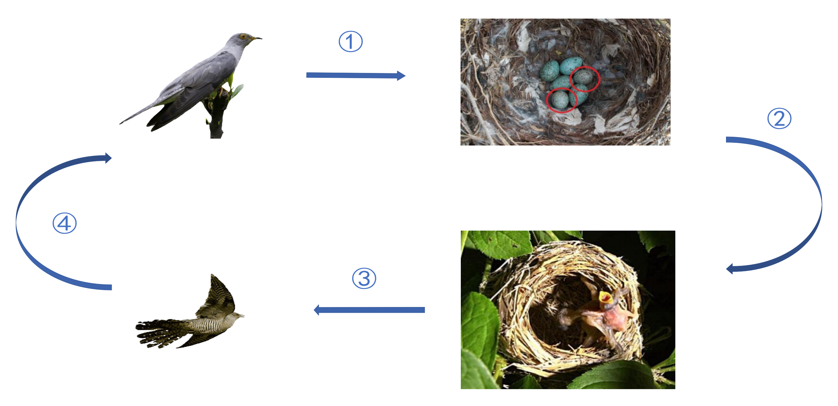
2.1. Cuckoo Breeding Behavior

CS is a heuristic algorithm proposed by Yang [22]. It is an intelligent algorithm that imitates the feeding method of cuckoos. As shown in Figure 1, cuckoo mothers choose other birds’ nests to lay eggs. In nature, cuckoo mothers prefer to choose the best nest among a plenty of nests [41]. In addition, baby cuckoos have some methods to ensure their safety. For one thing, some cuckoo eggs are pretty similar to those of hosts. Another thing is that the hatching time of the cuckoo is often earlier than those of the host birds. Therefore, once the little cuckoo breaks its shell, they have a chance to throw some eggs out of the nest to enhance their possibility of survival. Moreover, the little cuckoo can imitate the cry of the child of the host bird to get more food. However, the survival of a baby cuckoo is not easy. If the host recognizes the egg, it will be discarded. In that case, host mothers only choose to get rid of their eggs or abandon the nests altogether. Later, cuckoo mothers will move to build a new nest somewhere else. If the eggs are lucky enough not to be recognized, they will survive. Therefore, for the safety of the children, cuckoo mothers always choose some birds similar to their living habits [42].

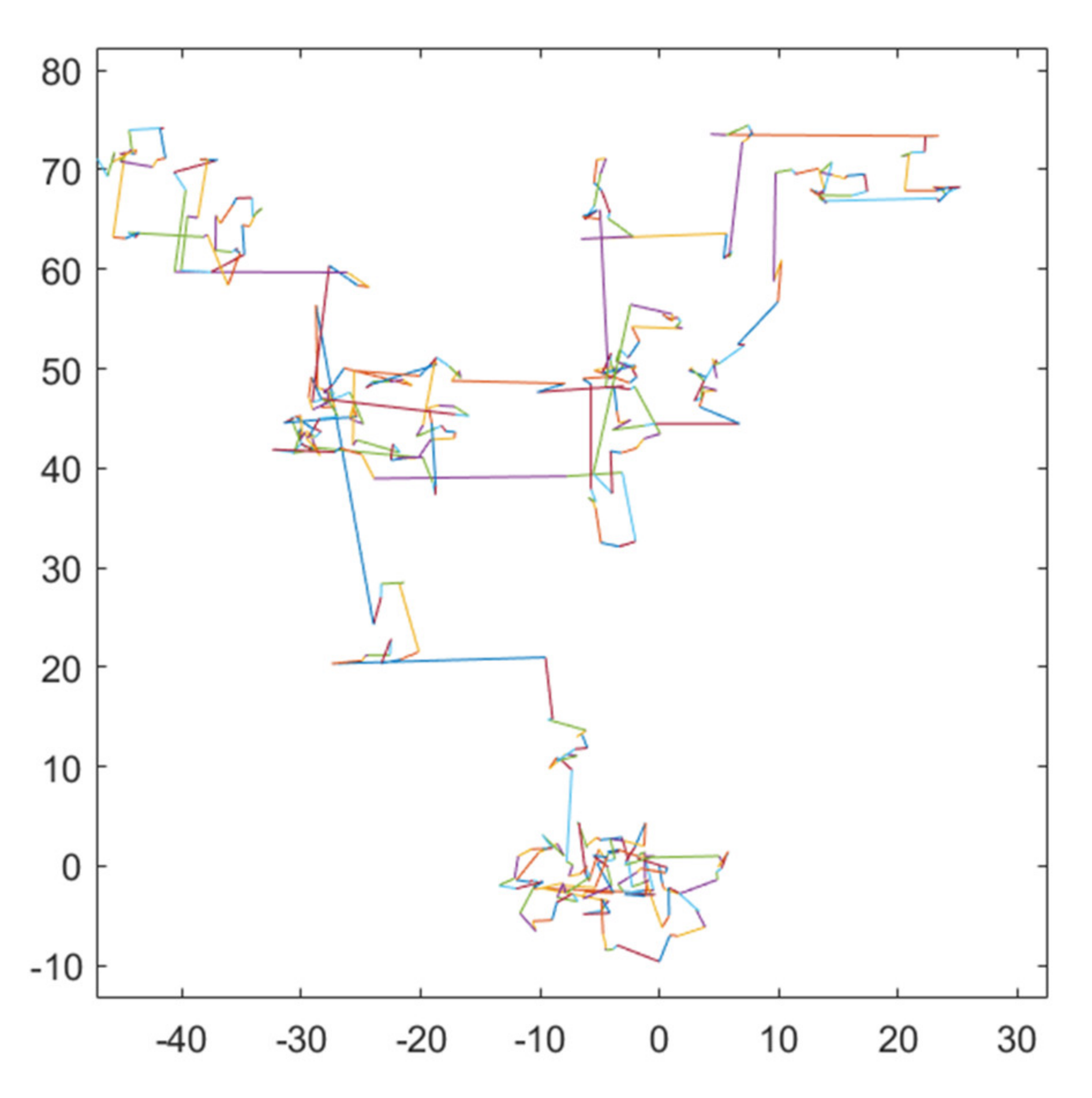
2.2. Lévy Flights Random Walk (LFRW)

There are some different methods to find the best solution for a local search in the conventional evolutionary algorithms. For example, Evolutionary Strategy (ES) [40] follows a Gaussian distribution. GA and evolutionary programming (EP) choose the random selection mode to find the best solution. A random searching measure is always a better choice in most heuristic algorithms. However, blindly random selection will only reduce the efficiency of the algorithm. Therefore, CS applies a new searching method to enhance itself. In a global search, CS adopts a new searching space technique, which is called $L\mathit{é}vy$ Flight Random Walk (LFRW). A quantity of evidence has confirmed that some birds and fish in nature use a mixture of $L\mathit{é}vy$ flight and Brownian motion to capture prey [43]. In a nutshell, $L\mathit{é}vy$ flight is the approach that combines long and short steps. The step length of $L\mathit{é}vy$ flight obeys $L\mathit{é}vy$ distribution. Sometimes, the direction of $L\mathit{é}vy$ flight will suddenly turn 90 degrees. Its 2D plane flight trajectory is simulated in Figure 2. In local search, CS adopts a novel measure called random walk [44]. As we all know, it is challenging to balance the breadth and depth when the population is in convergence. $L\mathit{é}vy$ flight has a promising performance in a searching space as it mixes long and short steps, which benefits global search. Random walk describes the behavior of random diffusion. Combining the two methods is beneficial to improve the depth and breadth of the algorithm, which is conducive to improving the accuracy of the algorithm.

In a word, $L\mathit{é}vy$ flight is a random walk that is used in the second stage of CS. The offspring is generated by $L\mathit{é}vy$ flight as follows:

$$\begin{gathered} X_i^{g+1}=X_i^g+\alpha \otimes L\mathit{é}vy\left(\beta \right) \\ \alpha ={\alpha }_0\otimes \left(X_i^g-X_k^g\right) \end{gathered}$$

(2)

where $X_i^{t+1}$ is the next generation, $X_i^t$ is the current generation, and $X_k^t$ is a randomly generated solution; $\alpha$ ($\alpha >0$) is the step size of $L\mathit{é}vy$ flight; $L\mathit{é}vy\left(s,\lambda \right)$ is a random search path following $L\mathit{é}vy$ distribution; $\otimes$ is a special multiplication indicating the entry-wise multiplication; and ${\alpha }_0$ is a step control parameter. Yang simplified the $L\mathit{é}vy$ distribution function and Fourier transform to obtain the probability density function in power form, which is given by:

$$L\mathit{é}vy\left(\beta \right)~\mu =t^{-1-\beta },0<\beta <2$$

(3)

Actually, the integral expression of $L\mathit{é}vy$ distribution is quite complex, and it has not been analyzed. However, Mantegna proposed a method to solve for random numbers with a positive distribution in 1994 [45], which is similar to the distribution law of $L\mathit{é}vy$ distribution. Thus, this method is used in Yang’s approach as follows:

$$L\mathit{é}vy\left(\beta \right)~\frac{u}{{\left|v\right|}^{\frac{1}{\beta }}}$$

(4)

where both $u,v$ follow the Gaussian normal distribution. The specific expressions are given by:

$$\begin{gathered} u~Norm\left(0,{\sigma }^2\right),v~Norm\left(0,1\right) \\ \sigma ={\left\{\frac{\mathsf{\Gamma }\left(1+\beta \right)\sin \left(\frac{\pi \beta }{2}\right)}{\beta \mathsf{\Gamma }\left(\frac{1+\beta }{2}\right)2^{\frac{\beta -1}{2}}}\right\}}^{\frac{1}{\beta }} \end{gathered}$$

(5)

Usually, $1<\beta \le 3$. In original CS, $\beta$ is set to 3/2 and $\mathsf{\Gamma }$ is a gamma function, which is formulated as:

$$\mathsf{\Gamma }\left(z\right)={{\displaystyle \int }}_0^{+\infty }\frac{t^{z-1}}{e^t}dt$$

(6)

Therefore, the calculated formula of the offspring is as follows:

$$X_i^{t+1}=X_i^t+{\alpha }_0\frac{u}{{\left|v\right|}^{\frac{1}{\beta }}}\left(X_i^t-X_k^t\right)$$

(7)

2.3. Local Random Walk

As is mentioned above, CS has two location updating methods for global and local searches. In global search, it adopts $L\mathit{é}vy$ flights to evolve the population. In local search, it adopts random walk to excavate potential information for solutions, which enhances the exploitation of CS. In this section, CS proposed a threshold that is called $P_a$. The application law of $P_a$ is:

$$u_i=\left\{\begin{array}{cc}{v}_i,\hfill & \hfill rand>P_a\\ x_i,\hfill & \hfill otherwise\end{array}\right.$$

(8)

where $x_i$ is the population generated by $L\mathit{é}vy$ Flight,$i$ is the position of the solution vectors in the population, and $v_i$ is a trial vector, which is obtained by the random walk of $x_i$. In general, CS enforces random walk only when the generated value satisfies the threshold $P_a$. Random walk of CS shall be carried out according to the following rules:

$$v_i=x_i+\alpha \otimes H\left(P_a-r\right)\otimes \left(x_m-x_n\right)$$

(9)

where $i$ means the index of the current solution in the population, $\alpha$ is the coefficient of the step size, $H$ is a Heaviside function, $r$ is a random number following a normal distribution, and $x_m$ and $x_n$ are both the two random solution vectors in the current population. In this way, the local optimization is more stable. Moreover, it is easy to obtain excellent solution information. Algorithm 1 shows the pseudo-code of CS.

Algorithm 1 The pseudo-code of CS

Input: $\mathit{N}$: the population size    $\mathit{D}$: the dimension of the population    $\mathit{G}$: the maximum iteration numbers    $\mathit{g}$: the current iteration    ${\mathit{P}}_{\mathit{a}}$: the possibility of being discovered

${\mathit{X}}_{\mathit{i}}$: a single solution in the population

${\mathit{X}}_{\mathit{b}\mathit{e}\mathit{s}\mathit{t}}:$ the best solution of all solution vectors in the current iteration

1: For $i=1:N$

2:  Initialize the $X_i$ 3: End

4: Calculate $f \left(X_i\right)$, find the best nest $X_{best}$ and record its fitness $f\left(X_{best}\right)$

5: While $g<G$ do

6:   Randomly choose $i$th solution to make a LFRW and calculate fitness $f\left(U_i\right)$

7:  If $f\left(U_i\right)\le f\left(X_i\right)$

8:   Replace $f\left(X_i\right)$ by $f\left(U_i\right)$ and update the location of the nest by Equation (2)

9:  End If

10: For $i$ = 1:$N$

11:  If the egg is discovered by the host

12:   Random walk on current generation and generate a new solution $V_i$ by Equation (9)

13:   If $f(V_i)\le f\left(X_i\right)$

14:    Replace $f\left(X_i\right)$ by $V\left(X_i\right)$ and update the location of the nest

15:   End If

16:  End If

17: End for

18: Replace $X_{best}$ with the best solution obtained so far

19: $g=g+1$

20: End while

Output: The best solution

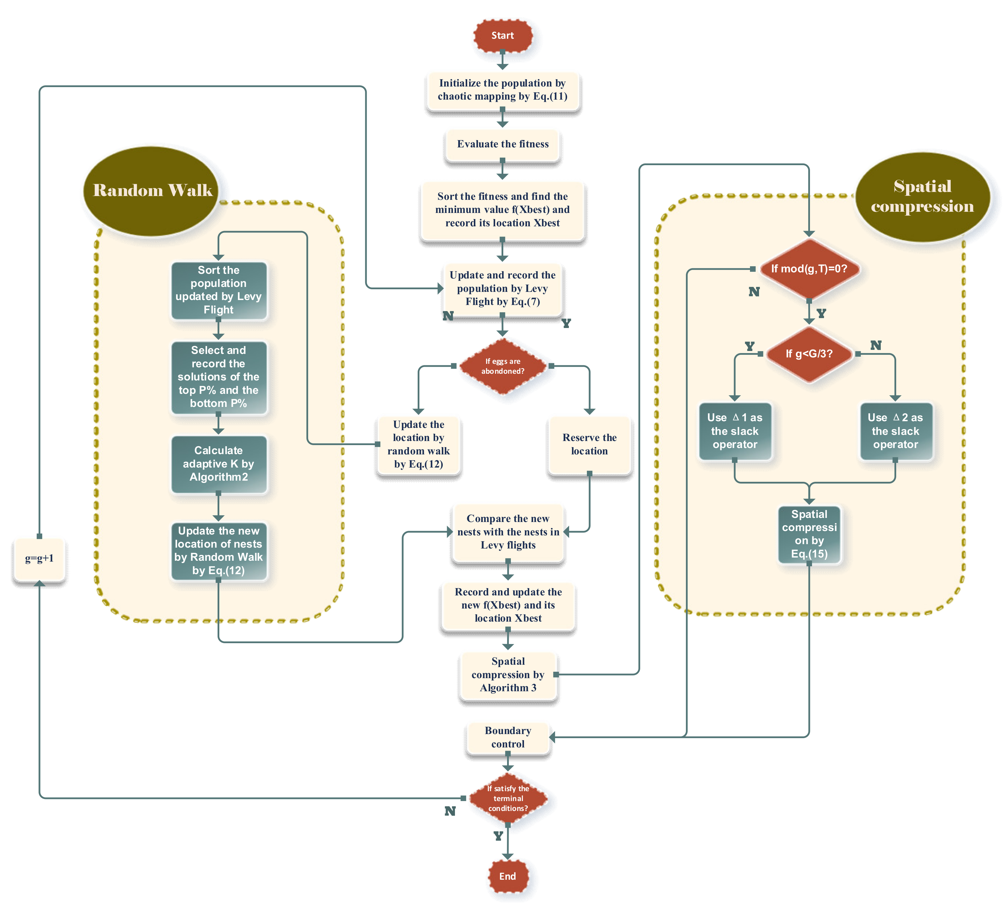
3. Main Ideas of Improved AGSCCS

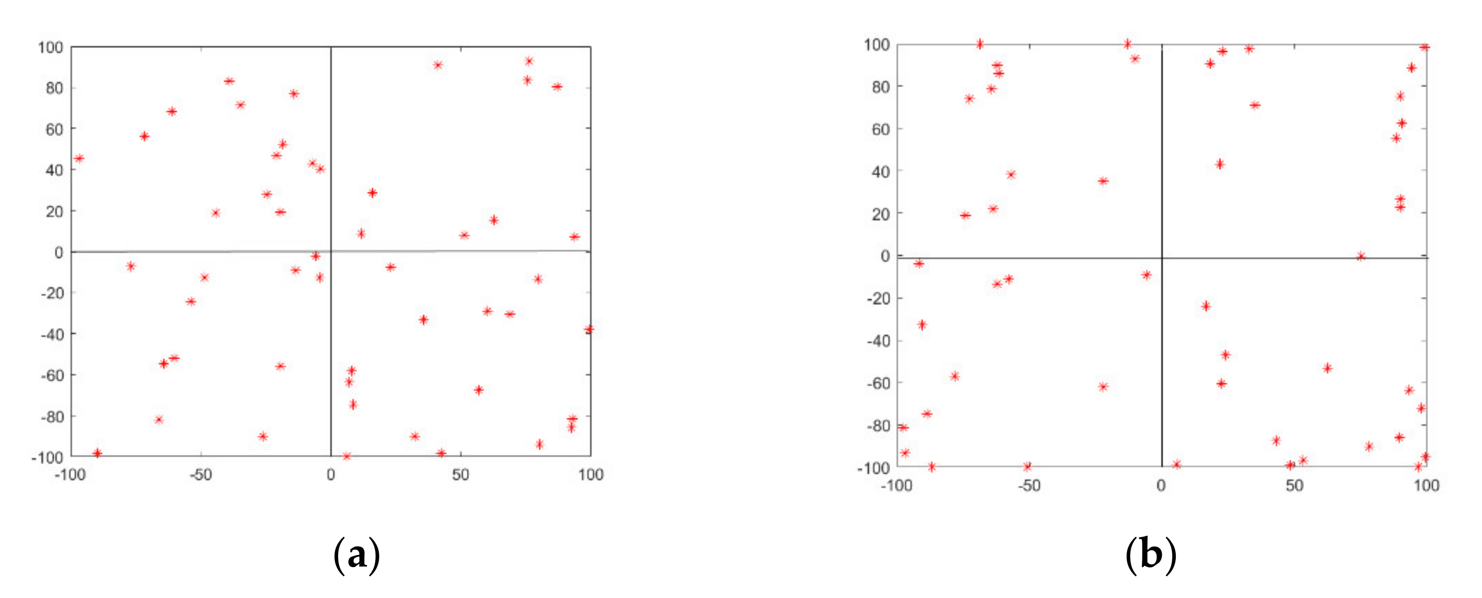
Although many attempts have been made to improve the performance of CS, there are still some disadvantages of CS because of its simple structure [23]. Firstly, the local search follows the pseudo-random number distribution in the original CS. In this case, the population cannot balance the global search and local search in the later stage due to the nonuniformity of the distribution in high-dimensional space, which will fall into a local optimization [46,47]. In other words, the exploration and exploitation ability of the algorithm will be limited due to the pseudo-random distribution. Secondly, the original CS uses a static method to calculate the step size, leading to slow convergence [48]. Thirdly, the global search capacity has been improved by $L\mathit{é}vy$ Flight. It uses the combination of long and short distances for spatial search and quickly determines the feasible region. However, the local search needs to be enhanced because of the uncertainty of random search, which may also cause the local optimal [24].

Based on the above problems, AGSCCS has been proposed. AGSCCS retains the core idea of the original CS algorithm and makes some adjustments to the drawback of CS. Firstly, it uses the chaotic mapping to generate the initial population instead of the pseudo-random distribution. This measure solves the problem of the nonuniformity of the distribution in high-dimensional space. Secondly, the generation step size is modified. An adaptive coefficient is added to control the change in the step size. A guided sorting method is added to make full use of the optimum group and worst group. This measure solves the defect of the imbalance between exploration and exploitation in the later period, giving an excellent promotion for the exploitation. Thirdly, a SC technique is also proposed. It mainly aims at quickly determining the vicinity of the ideal solution and prevents the population from falling into the local optimal. The following sections introduce the three above strategies.

3.1. Initialization

The standard evolutionary algorithms will tend to appear premature because of the decline in population diversity and the setting of control parameters in the later stage [49]. The randomly generated initial population can easily cause population convergence and aggregation. The chaotic mapping method is used to initialize the population to improve the effectiveness and universality of the CS algorithm. Chaos is a common nonlinear phenomenon, which can traverse all states and generate chaotic sequences without repetition in a specific range [50]. Compared with the traditional initialization, the chaotic mapping method preferentially selects the position and velocity of particles in the initialization population. It can also use the algorithm to randomly generate the initial value of the population, which maintains the diversity of the population and makes full use of the space and regularity of the initial ergodic of chaotic dynamics.

As can be seen from Figure 3, the initial population generated by using Logistic chaotic initialization mapping is more uniform. Assuming that the (0,0) point is the segmentation point, the whole search domain is divided into four spaces. Points 13, 9, 12, 16 are randomly generated in the four quadrants by common initialization, and the initial populations for 11, 13, 12, 14 are generated by the chaotic mapping method. From the distribution’s point of view, the initial population generated by the chaotic mapping method is more uniform.

Common chaotic mapping models include piecewise linear tent mapping, chaotic characteristics of a one-dimensional Iterative Map with Infinite Collapses (ICMIC), sinusoidal chaotic mapping (sine mapping), etc. [50,51]. However, the tent chaotic map has unstable periodic points, which easily affects the generation of chaotic sequences. The pseudo-random number generated by the ICMIC model is between [−1,1], which does not meet the initialization value required in this paper. The scope of the application of the sine mapping function also has significant limitations. Its independent variables and value range are often controlled between [−1,1]. To simplify the model and improve the efficiency of the algorithm, we will adopt a logistic nonlinear mapping after considering the above factors. The logical mapping can be described as:

$$y_i^{g+1}=\mu y_i^g\left(1-y_i^g\right)$$

(10)

where $y_i$ is a random value that follows a uniform distribution,$i$ means the current position of the current solution vector in the population, $g$ is the current iteration, and $\mu$ is the control coefficient of the expression, and it is a positive constant. The value of $g$ is a positive integer, which indicates the current number of iterations. When 3.5699 ≤ $\mu$ ≤ 4, the system is in full chaos and has no stable solution [2]. Therefore, the population initiation is given as:

$$X_i^0=(X_{max}-X_{min})\ast y_i^1+X_{min}$$

(11)

where $y_i^1$ is an initial value generated by the chaotic map according to Equation (10), and $X_{max}$ and $X_{min}$ are the upper and lower limits of the search space, respectively.

3.2. A Scheme of Updating Personalized Adaptive Guided Local Location Areas

In nature, if the host does not find the cuckoo’s eggs, the eggs can continue to survive. Once the cuckoo’s eggs are found, they will be abandoned by the host and the cuckoo’s mother can only find another nest to lay eggs. In the CS algorithm, the author proposed a ‘random walk’ method. $P_a$ is the probability of the eggs being discovered. Once found, these solutions need to be transferred randomly and immediately to improve their survival rate. The total number of solutions in each iteration remains unchanged [52]. The above process is the random walk. However, any random behavior can affect the accuracy of the algorithm. The global optimal may be missed if the step size is too long. Meanwhile, if the step size is too short, the population will always search around the local optimal. Thus, an adaptive differential guided location updating strategy is proposed to avoid this situation.

Intuitively, a completely random step size is risky for the iteration because it may run counter to the direction of the solution. The common method is to use the information of excellent solutions to pass on to the next generation to generate children [53,54]. Literature [38] adopts a new variation rule. It uses two randomly selected vectors coming from the top and bottom 100$p\%$ individuals in the current size population, and the third vector is randomly selected from the middle [$NP-2 \left(100p\%\right)$] individuals ($NP$ is the population size). The three groups set the balance between the global search ability and local development tendency and improve the convergence speed of the algorithm. In this study, we combine this improvement concept with CS.

The original CS always uses the pseudo-random number method to generate a new step size in the local search phase. However, pseudo-random numbers are easy for showing the nonuniformity, especially in high-dimensional space. In some literature [55,56], researchers often used the information of the optimal solution and the worst solution in the previous generation solution set to replace the random step-size, which can make full use of the information of the solution. However, suppose we only use the single optimal solution and the worst solution in each generation of the population. In that case, the population may fall into local stagnation because of following the direction of the optimal solution. Therefore, the definitions of ‘optimal solution group’ and ‘worst solution group’ are proposed. The optimal solution group is the top 100$p\%$ individuals, while the worst solution group is the bottom 100$p\%$ individuals in the current $NP$ size population. The advantage of using a solution group instead of an optimal solution is to avoid always following the same iterative direction of the optimal solution. This specific idea can refer to Figure 3 (②). Furthermore, this measure contributes to the diversity of the population, which is beneficial to the iteration in the latter stage. The formula is described as follows:

$$nes{t}_i^{g+1}=nes{t}_i^g+K·\left(nes{t}_{pbest}^g-nes{t}_{pworst}^g\right)$$

(12)

where nest is the iterative population, $g$ is the current iteration, $i$ means the position of the decision vector in population, $pbest$ and $pworst$ are the top and bottom $p\%$ solutions in population, and $K$ is a coefficient of controlling step size. The core idea of this method is: (1) for each population, we can learn the information of the best solution group and the worst solution group from the current generation. (2) The effect of difference is understood as the positive effect of the best solution group and the negative effect of the worst solution group. In the iterative process, the variation direction of the offspring follows the same direction as the best solution group vector while maintaining the opposite direction to the worst solution group of the random vector. The specific optimization direction of the offspring will be determined by the parent and the variation direction. This specific idea will be visualized in Figure 3.

Figure 4 shows the specific ideas for population evolution—where a is the current optimal solution, b is current worst solution, and c is the parent solution. In some improvements of CS, researchers utilize a and c to generate the offspring. However, they do not notice that the worst group affects the iteration at the same time. It will make the population evolve along the direction of the optimal solution and lead to falling into local optimization. In our method, a and b will firstly generate the direction of the next generation variation direction. Then, the parent will combine with the variation direction to produce a new searching direction.

Moreover, the adjustment for the operator $K$ is also essential. The best solution group and the worst solution group previously proposed are used to control the direction of the iteration step, and $K$ is the coefficient controlling this iteration step. Its randomness will also affect the efficiency of the algorithm. Our idea is to control the size of $K$ so that the algorithm maintains a relatively large step size at the beginning of the iteration, and it could quickly converge near the ideal solution. In the later stage, we will gradually reduce the step size to converge to the position of the ideal solution accurately. In this study, we proposed an adaptive method to control $K$. The pseudo-code can be shown in Algorithm 2.

Algorithm 2 The pseudo-code of $K$

Input: $\mathit{g}$: the current iteration

$\mathit{G}$: the maximum number of iterations

1: $K_{max}=1,K_{min}=0.1$

2: Initialize $K$, $K_0=0.4$

3: $\lambda =e^{1-\frac{g}{G+1-g}}$

4: Update $K\prime$, $K\prime =K_0\ast 2^{\lambda }$

5: Judge whether the current $K$ is within the threshold

6: If rand < threshold do

7:   $K=K_{min}+\mathrm{rand}\ast K_{max}$

8: Else

9:   $K=K\prime$ 10: End if 11: Calculate new step size by Equation (12)

Output: The value of $stepsize$

$K$ is a parameter for the step size. It can be seen from Algorithm 2 that the value of $K$ increases during iteration. In the beginning, the value of the vector $K$ is close to $2K_0$, which is convenient for the population, thereby accelerating the convergence of the optimal solution. In the later stage, $K$ gradually decreases into $K_0$, which prevents excessive convergence. The above measure can ensure the algorithm is searching around the feasible areas all along. The threshold is set to appropriately increase the diversity of the algorithms and reduce the possibility of searching for the local optimal. It allows random change for the step size, which increases the diversity of the algorithm. Thus, the population variety remains in the later stage.

3.3. Spatial Compressions Technique

Original CS uses simple boundary constraints, which have no benefits for spatial convergence. In this section, a SC technique is proposed to actively adjust the optimization space. Briefly, its primary function is to properly change the optimization space of the algorithm in the iterative process. In the evolutionary early stage, the algorithm space is compressed to converge near the ideal solution quickly. In the late stage of evolution, the behavior of the compressing space will be slowed down appropriately to prevent a fall into the local optimal [40].

SC should cooperate with the optimization population convergence. The shrinkage operator is set larger than the one in the later stage. Therefore, the population can quickly eliminate the infeasible area in the beginning. In the later stage, the shrinkage operator should be set smaller to improve the convergence accuracy of the algorithm. Based on the above methods, we propose two different shrinkage operators for the different stages according to the current population. The first operator accelerates the population searching around the space used in the beginning stage. The second one is used to improve the accuracy of the algorithm and find more potential solutions.

$$\Delta 1=0.5\ast X_{max}-X_{min}$$

(13)

$$\Delta 2=\frac{\beta \ast u_i^t-l_i^t-\left(X_{max}-X_{min}\right)}{2}$$

(14)

where $X_{max} \mathrm{and} X_{min}$ represent the upper and lower bounds of the ith decision variable in the population, $u_i^t$ and $l_i^t$, respectively, represent the actual limit of the decision variable in the current generation, $\beta$ is a zoom parameter, and $D$ is the dimension of the population. According to the above operators, Equation (13) is used in the beginning stage and Equation (14) is used later. In this article, the first third of the iteration is the beginning stage and the last two-thirds are the later stage. Based on the above analysis and some improvements, the new boundary calculation formula is as follows:

$$u_i^{t+1}=X_{max}+\Delta ;l_i^{t+1}=X_{min}-\Delta$$

(15)

where Δ is a shrink operator. It has different values depending on the current iteration. The pseudo-code of the section of the SC technique is shown in Algorithm 3.

Algorithm 3 The pseudo-code of shrink space technique

Input: $\mathit{g}$: the current iteration

$\mathit{G}$: the maximum number of iterations

$\mathit{N}$: the population size

1: Initialize $\mathsf{\Delta }$, $T=20$

2: If mod (g$,T$) = 0

3:  For $g=1$ to $G$ do

4:   Calculating $\mathsf{\Delta }1$ and $\mathsf{\Delta }2$ for different individuals in the population by Equations (13) and (14)

5:   If $g$ < $G/3$ do

6:    choose $\mathsf{\Delta }1$ as shrinking operator

7:   Else

8:    choose $\mathsf{\Delta }2$ as shrinking operator 9:   End if

10:  End for

11: Update the new upper and lower bounds by Equation (15)

12: End if

Output: new upper and lower bounds

There is no need to shrink the space frequently, which is likely to cause over-convergence. Given this, we choose to perform a spatial convergence every 20 generations. It will not only ensure the efficiency of the algorithm, but also effectively save computing resources. The pseudo-code and flow diagrams of AGSCCS are presented in Algorithm 4 and Figure 5.

Algorithm 4 The pseudo-code of AGSCCS

Input: $\mathit{N}$: the population size

$\mathit{D}$: the dimension of decision variables

$\mathit{G}$: the maximum iteration number

${\mathit{P}}_{\mathit{a}}$: the possibility of being discovered

${\mathit{X}}_{\mathit{i}}$: a single solution in the population

${\mathit{X}}_{\mathit{b}\mathit{e}\mathit{s}\mathit{t}}:$ the best solution of the all solutions in the current iteration

1: For $i=1:N$

2:  Initialize the population $X_i^0$ by Equation (11) 3: End

4: Calculate $f \left(X_i^0\right)$, find the best nest $X_{best}$ and record its fitness $f\left(X_{best}\right)$

5: While $g<G$ do

6:  Make a LFRW for $X_i$ and calculate fitness $f\left(X_i\right)$

7:  If $f\left(U_i\right)\le f\left(X_i\right)$

8:   Replace $f\left(X_i\right)$ with $f\left(U_i\right)$ and update the location of the nest

9:  End If

10:  Sort the population and find the top and bottom $p\%$

11:  If the egg is discovered by the host

12:   Calculate the adaptive step size by Algorithm 2 and Equation (12)

13:    Random walk on current generation and generate a new solution $V_i$

14:  End If

15:  If $f\left(V_i\right)\le f\left(X_i\right)$

16:    Replace $X_i$ with $V_i$ and update the location of the nest

17:  End If

18: Replace $X_{best}$ with the best solution obtained so far

19:  If $mod \left(t, T\right)=0$

20:    Conduct the shrink space technique as shown in Algorithm 3

21:    If the new boundary value is not within limits

22:     Conduct boundary condition control

23:    End if

24:   End if

25: $g=g+1$

26: End while

Output: The best solution after iteration

3.4. Computational Complexity

If $N$ is the wolf pack size, then $D$ is the dimension of the optimization problem and $M$ is the maximum iteration number. The computational complexity of each operator of AGSCCS is given below:

(1)

The chaotic mapping of AGSCCS initialization in $O\left(N\right)$ time.

(2)

Adaptive guided local location areas require $O\left(2\right)$ time.

(3)

Adaptive operator F requires $O\left(N\right)$ time.

(4)

The shrinking space technique demands $O(\frac{M}{T}\times D)$, where T is the threshold controlling spatial compress technique.

In conclusion, the time complexity of each iteration is $O(2$N$+2+\frac{M}{T}\times D)$. As $2N$ is more than two, the overall time complexity of the proposed AGSCCS algorithm can be expressed as $O(2N+\frac{MD}{T})$. Therefore, the total computational complexity of AGSCCS is equal to $O\left(\left(2N+\frac{MD}{T}\right)\times M\right)$ for the maximum iteration number $M$.

4. Experiment and Analysis

In this section, some experiments will be performed to examine the performance of AGSCCS. To make a comparison, the test will be done on the other algorithms, including CS [22], ACS, ImCS, GBCS, and ACSA at the same time. All of them improve the original CS algorithm from different angles. For example, ACS changes the parameters in the random walk method to increase the diversity of the mutation [25]. GBCS combines the process of a random walk with PSO, which realizes adaptive controlling and updating of parameters through external archiving events [27]. ImCS draws on the opposite learning strategy and combines it with the dynamic adjustment of score probability [32]. ACSA is another improved CS algorithm that adjusts the generating step size [31]. It uses the average value, maximum, and minimum to calculate the next generation’s step size.

4.1. Benchmark Test

The benchmark test is a necessary part of the algorithm. It can verify both the performance and characteristics of the algorithm. During these years, lots of benchmark tests have been proposed. In this paper, CEC2014 will be adopted to examine the algorithm. It is a classic collection of the test function, including Ackley, Schwefel’s, Rosenbrock’s, Rastrigin’s, etc. [57]. It covers 30 benchmark functions. In general, these 30 test functions can be summarized as four parts:

(1)

Unimodal Functions ($F_1-F_3$)

(2)

Simple multimodal Functions ($F_4-F_{16}$)

(3)

Hybrid functions ($F_{17}-F_{22}$)

(4)

Composition functions ($F_{22}-F_{30}$)

The specific content of each function has been listed in a lot of research [58].

4.2. Comparison between AGSCCS and Other Algorithms

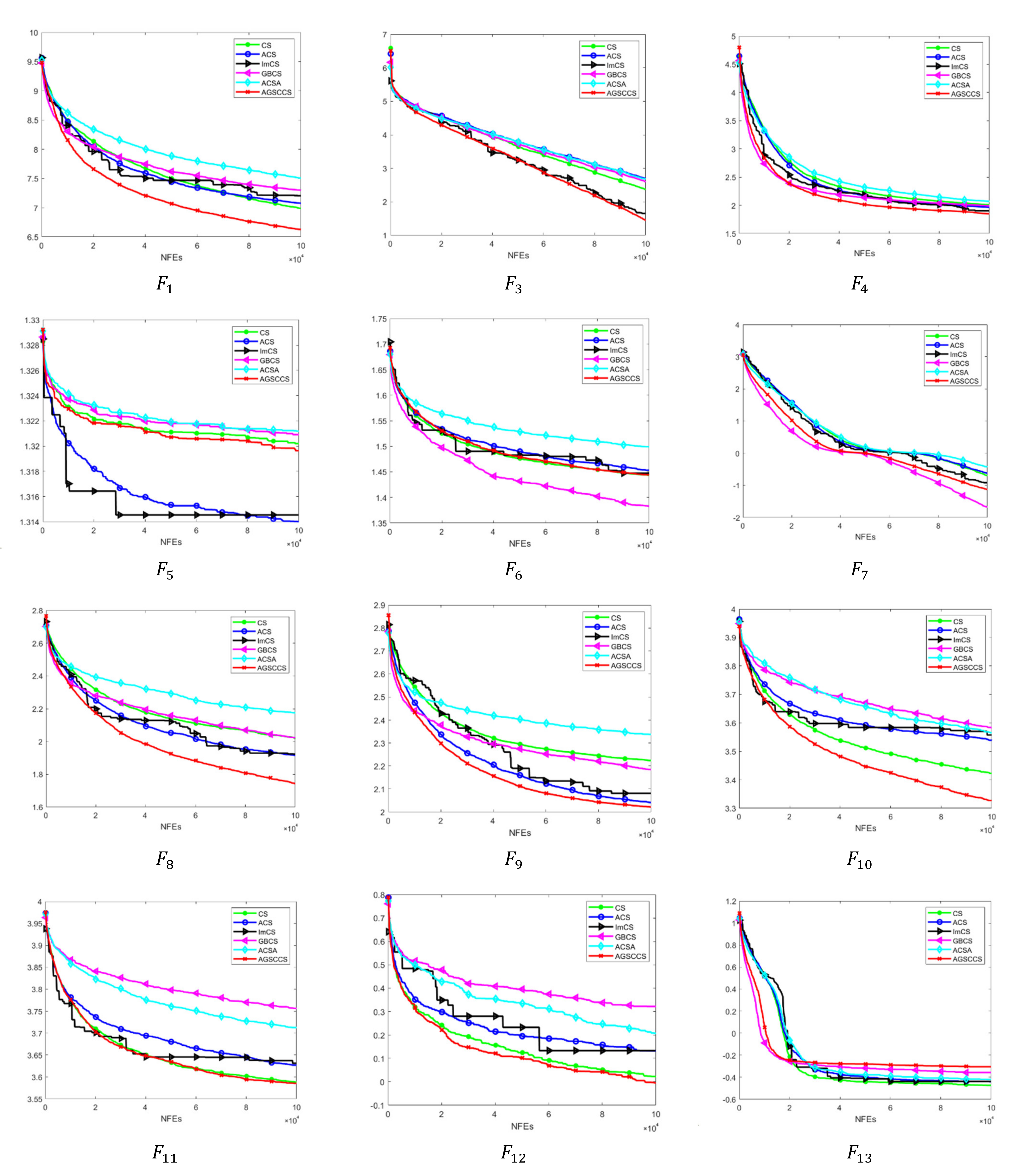
CS is a heuristic algorithm that was proposed in recent years. Given this, in order to test its performance comprehensively, we chose four differently related CS algorithms to make the comparison.

The population size is set to $N=50,$ and the dimension of the problems is set to $D=30$. The function evaluation times are set to FES = 100,000. Each experiment is run 30 times and six algorithms are completed to get the mean and standard values.

To comprehensively analyze the performance of AGSCCS, five relevant algorithms were chosen: CS, ACS, ImCS, GBCS, and ACSA. In this study, the population size of each algorithm is set to 30. Thirty turns tests would be run to avoid any randomness caused by one turn. The experimental results show both the mean and standard values of all the experiments in

Table 1. Experimental results of CS, ACS, ImCS, GBCS, ACSA, and AGSCCS at $D=30$. (Bold is the optimal algorithm results of each test function.)

	CS		ACS		ImCS		GBCS		ACSA		AGSCCS
	Mean	Std	Mean	Std	Mean	Std	Mean	Std	Mean	Std	Mean	Std
f1	9.76 × 106	2.42 × 106	1.19 × 107	3.35 × 106	1.60 × 107	2.34 × 105	1.99 × 107	5.97 × 106	3.21 × 107	1.05 × 107	4.23 × 106	1.40 × 106
f2	1.00 × 1010	0.00	1.00 × 1010	0.00	1.00 × 1010	0.00	1.00 × 1010	0.00	1.00 × 1010	0.00	1.00 × 1010	0.00
f3	2.31 × 102	8.32 × 101	4.98 × 102	1.34 × 102	4.49 × 101	1.98 × 101	3.99 × 102	9.55 × 101	4.76 × 102	2.10 × 102	2.80 × 101	7.34
f4	1.02 × 102	1.87 × 101	9.24 × 101	2.54 × 101	7.94 × 101	2.29 × 101	9.79 × 101	1.80 × 101	1.18 × 102	2.12 × 101	7.08 × 101	2.28 × 101
f5	2.09 × 101	8.99 × 10−2	2.06 × 101	5.57 × 10−2	2.06 × 101	4.87 × 10−2	2.09 × 101	5.06 × 10−2	2.09 × 101	5.56 × 10−2	2.09 × 101	7.94 × 10−2
f6	2.77 × 101	9.62 × 10−1	2.84 × 101	2.29	2.80 × 101	2.39	2.42 × 101	3.36	3.16 × 101	1.69	2.78 × 101	1.32
f7	2.03 × 10−1	5.60 × 10−2	2.35 × 10−1	7.40 × 10−2	1.20 × 10−1	5.70 × 10−2	2.12 × 10−2	1.30 × 10−2	3.70 × 10−1	9.40 × 10−2	7.51 × 10−2	5.61 × 10−2
f8	1.04 × 102	1.44 × 101	8.24 × 101	1.41 × 101	8.39 × 101	1.30 × 101	1.05 × 102	1.54 × 101	1.49 × 102	1.69 × 101	5.53 × 101	8.21
f9	1.67 × 102	2.16 × 101	1.10 × 102	1.55 × 101	1.21 × 102	1.42 × 101	1.53 × 102	1.46 × 101	2.18 × 102	1.80 × 101	1.05 × 102	1.48 × 101
f10	2.65 × 103	1.81 × 102	3.45 × 103	4.12 × 102	3.61 × 103	4.40 × 102	3.83 × 103	5.35 × 102	3.68 × 103	4.45 × 102	2.12 × 103	1.96 × 102
f11	3.87 × 103	1.91 × 102	4.23 × 103	5.23 × 102	4.28 × 103	3.90 × 102	5.70 × 103	4.25 × 102	5.16 × 103	2.14 × 102	3.85 × 103	2.67 × 102
f12	1.05	1.23 × 10−1	1.36	2.29 × 10−1	1.36	2.34 × 10−1	2.10	3.45 × 10−1	1.61	2.18 × 10−1	9.89 × 10−1	1.43 × 10−1
f13	3.37 × 10−1	4.61 × 10−2	3.64 × 10−1	3.85 × 10−2	3.66 × 10−1	4.43 × 10−2	4.40 × 10−1	5.97 × 10−2	3.81 × 10−1	5.12 × 10−2	4.97 × 10−1	5.75 × 10−2
f14	2.70 × 10−1	2.67 × 10−2	2.68 × 10−1	2.83 × 10−2	2.79 × 10−1	2.97 × 10−2	3.00 × 10−1	3.44 × 10−2	2.62 × 10−1	2.14 × 10−2	4.31 × 10−1	2.80 × 10−1
f15	1.47 × 101	1.38	1.78 × 101	1.81	1.66 × 101	1.52	1.61 × 101	1.41	1.82 × 101	1.36	1.07 × 101	1.01
f16	1.27 × 101	1.72 × 10−1	1.28 × 101	1.89 × 10−1	1.28 × 101	2.09 × 10−1	1.27 × 101	1.97 × 10−1	1.27 × 101	3.91 × 10−1	1.27 × 101	2.34 × 10−1
f17	9.32 × 104	3.24 × 104	1.11 × 105	4.40 × 104	2.87 × 104	3.86 × 102	1.99 × 105	6.36 × 104	2.44 × 105	1.02 × 105	2.72 × 104	7.89 × 103
f18	3.69 × 103	4.06 × 103	3.12 × 104	1.55 × 104	3.60 × 102	1.42 × 102	2.17 × 103	1.25 × 103	3.11 × 103	3.66 × 103	3.33 × 108	1.83 × 109
f19	1.10 × 101	6.24 × 10−1	9.83	6.15 × 10−1	9.91	5.67 × 10−1	9.88	8.77 × 10−1	1.16 × 101	2.13	9.83	1.58
f20	3.21 × 102	5.94 × 101	3.86 × 102	9.66 × 101	3.76 × 102	1.75 × 101	3.69 × 102	1.13 × 102	7.06 × 102	1.72 × 103	1.65 × 102	3.27 × 101
f21	5.08 × 103	1.08 × 103	8.29 × 103	1.67 × 103	3.53 × 103	1.80 × 102	1.41 × 104	5.17 × 103	1.29 × 104	4.31 × 103	2.54 × 103	4.35 × 102
f22	3.45 × 102	9.51 × 101	2.87 × 102	1.12 × 102	3.08 × 102	7.07 × 101	2.31 × 102	9.23 × 101	4.45 × 102	1.79 × 102	2.64 × 102	1.15 × 102
f23	3.15 × 102	2.59 × 10−3	3.15 × 102	1.10 × 10−2	3.15 × 102	4.61 × 10−3	3.15 × 102	3.54 × 10−4	3.15 × 102	4.27 × 10−5	3.15 × 102	1.49 × 10−1
f24	2.34 × 102	4.11	2.34 × 102	3.50	2.33 × 102	3.34	2.29 × 102	5.04	2.31 × 102	2.09	2.28 × 102	2.09
f25	2.12 × 102	1.23	2.11 × 102	2.18	2.07 × 102	1.26	2.12 × 102	1.61	2.14 × 102	1.83	2.06 × 102	1.23
f26	1.00 × 102	4.02 × 10−2	1.00 × 102	4.05 × 10−2	1.00 × 102	3.44 × 10−2	1.00 × 102	6.63 × 10−2	1.00 × 102	7.58 × 10−2	1.00 × 102	8.99 × 10−2
f27	4.34 × 102	1.07 × 101	4.24 × 102	6.68	4.19 × 102	1.22 × 101	6.43 × 102	1.93 × 102	6.45 × 102	2.02 × 102	8.25 × 102	2.12 × 102
f28	1.06 × 103	4.33 × 101	1.03 × 103	4.44 × 101	1.03 × 103	5.14 × 101	9.41 × 102	3.91 × 101	8.68 × 102	2.68 × 102	1.03 × 103	1.19 × 102
f29	4.31 × 103	1.99 × 103	7.85 × 103	3.10 × 103	2.05 × 103	5.96 × 102	2.83 × 105	1.53 × 106	3.46 × 102	9.98 × 101	5.85 × 106	4.59 × 106
f30	4.93 × 103	9.64 × 102	5.96 × 103	2.56 × 103	3.16 × 103	7.30 × 102	3.81 × 103	8.84 × 102	1.68 × 103	2.09 × 102	3.62 × 103	1.32 × 103
+/−/≈	22/3/5		22/4/4		18/8/4		17/8/5		19/6/5		-

. The mean values show the precision performance, while the standard value shows the stability. According to the instruction of the CEC2014 benchmark tests, different kinds of functions are exhibited to verify the performance of the algorithms. For example, the unimodal function can reflect the exploitation capacity while the multimodal function shows the exploration capacity.

(1)

Unimodal functions ($F_1-F_3$). In Table 1, AGSCCS shows better performances in two functions in a group of three algorithms compared with CS, ACS, ImCS, GBCS, and ACSA when D = 30. Actually, except for function $F_2$, it may be because the CS algorithm cannot find the best value for the function, whereas AGSCCS always gets the best results in $F_1$ and $F_3$ compared to the other four algorithms. Given that the whole domain of the unimodal function is smooth, it is easy for the algorithm to find the minimum on the unimodal function. In this situation, AGSCCS can also score the best grades that prove the pretty exploitation capacity compared to other algorithms. This may owe to the SC technique. It quickly distinguishes the current environment to the extreme value of the region. Additionally, it benefits the capacity for algorithm convergence.

(2)

Simple multimodal functions ($F_4-F_{16}$). These functions are comparatively difficult for iterations compared to unimodal functions, given that they have more local extremums. In a total of 13 functions, AGSCCS performs better compared to eight functions, while CS, ACS, ImCS, GBCS, and ACSA have outstanding performances in functions 2, 1, 1, 3, 2, respectively; especially $F_{15}$ shown in Figure 6, given that it is a shifted and rotated expanded function with multiple extreme points. Moreover, it adds some characteristics of the Rosenbrock function into the search space, which strengthens the difficulty for finding the solution. AGSCCS achieves good iterative results on this function, which shows an excellent exploration capacity. This good exploration capacity is from the adaptive guided updating location method. The guided differential step size method can help the algorithm search for the direction of good solutions while avoiding bad solutions.

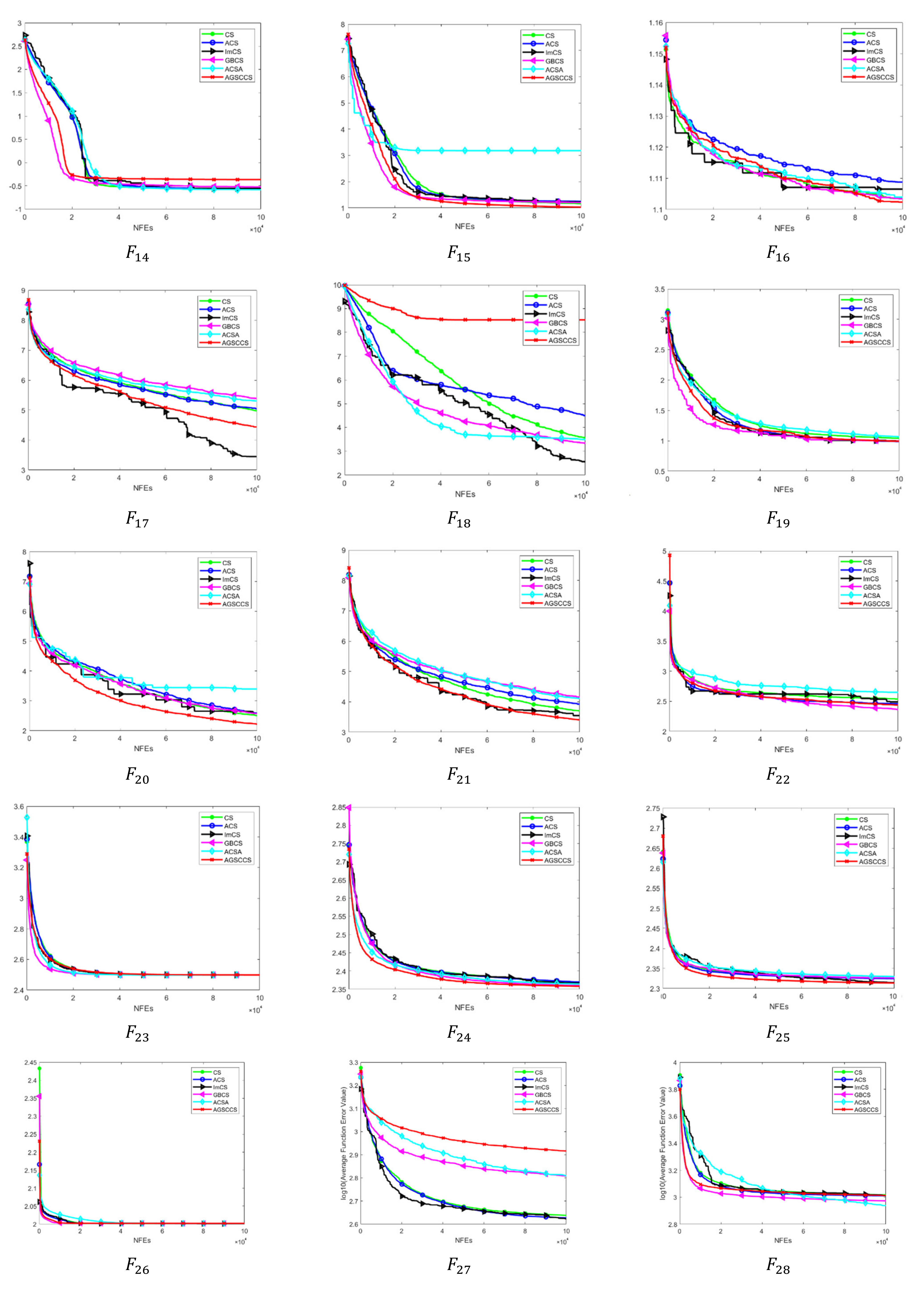
(3)

Hybrid functions ($F_{17}-F_{22}$). In these functions, AGSCCS still achieves the best compared to the other four algorithms. It has better performances on $F_{17}$, $F_{19}$, $F_{20}$, and $F_{21}$. In the total of six functions, CS, ACS, ImCS, GBCS, and ACSA lead in only functions 0, 1, 1, 2, 0. In $F_{20}$, the six algorithms almost converge to smaller values while AGSCCS can converge to a better value, which exhibits the excellent capacity of exploration of AGSCCS. Although GBCS has better results in $F_{22}$, AGSCCS is extremely close to its results. These experimental results can prove the leading position of AGSCCS in hybrid functions.

(4)

Composition functions ($F_{22}-F_{30}$). In $F_{22}-F_{30}$, AGSCCS shows better performances in four functions in total. Intuitively, AGSCCS has the best results in $F_{23}-F_{26}$. In these four functions, it always gets full marks. Although ACS performs unsatisfactorily on $F_{27}-F_{30}$, it cannot deny its excellent exploration and exploration ability. On the previous unimodal and multimodal functions, the comprehensive performances of ACS have been certified. The poor performances of ACS may be due to the instability of its state under multi-dimensional and multimodal problems. Therefore, AGSCCS does not show any disadvantages compared with the other four algorithms in hybrid composition functions.

To further analyze the searching process of AGSCCS, the iterative graphs for the CEC2014 benchmark are as follows.

Given that there is a considerable statistical difference between each function, we take the logarithm of the obtained function values to get the iterative graph. As can be seen from Figure 7, in 19 of the 30 test functions AGSCCS performs better than CS, ACS, ImCS, GBCS, and ACSA in terms of accuracy and stability. On the one hand, 19 functions of AGSCCS reach the minimum fitness value in the mean of iteration results, which is the algorithm with the largest number of minimum values among the six algorithms. This is due to the chaotic initialization and adaptive guided population iteration. The method of chaotic initialization improves the diversity of the population. The best and worst solution group of the previous generation are retained to provide references for the next generation and improve the exploration ability of the population, thus obtaining a smaller adaptation value. However, on the other hand, the AGSCCS algorithm performs equally well with the mean error. Compared with the second ImCS algorithm, AGSCCS achieves a minimum error on 20 test functions, while the second ImCS algorithm only shows better results on 5 test functions. This is due to the method of shrinking space. This method actively compresses the space in proper time, reduces the optimization range, improves the convergence speed, and enhances the stability of the algorithm. Similarly, in terms of convergence speed, AGSCCS’s convergence is faster than CS, ACS, ImCS, GBCS, and ACSA. In the same iteration, AGSCCS always tends to achieve a smaller value. There is no doubt that the SC technique contributes to the fast speed of convergence. In $F_6$, even if GBCS achieves the best solution compared with other algorithms within a relatively short time, it still $F_{10}$ , $F_{11}$ , and $F_{12}$ , which belong to the multimodal functions. Hence, it is not hard to conclude that GBCS has a worse iteration capacity than AGSCCS. Due to the SC technique, AGSCCS can easily and quickly find the optimal value in the searching space. The adaptive random replacement nest step ensures that the searching direction is not easy to fall into the local optimal. Therefore, in terms of comprehensive strength, the AGSCCS algorithm performs better.

In summary, it isn’t easy to find the best solution to perfectly solve all kinds of problems, whether it is through the original CS or some improved method. Therefore, the proposed AGSCCS is hard to find at all of the optimal solutions simultaneously. However, according to the above analysis, it can be seen that AGSCCS is a noteworthy method for optimization problems. It vastly improves the performance of the conventional CS on various issues, no matter if the problems are unimodal or multimodal. Furthermore, it shows better results than CS, ACS, ImCS, GBCS, and ACSA. AGSCCS adopts chaotic mapping generation and adaptive guided step size to avoid local stagnation. SC accelerates the speed of convergence. Three methods contribute to a stable balance between the exploitation and exploration capacity for AGSCCS.

4.3. Discussion

A sensitivity test will be done to verify the validity of the three improved strategies. It covers four experimental subjects called AGSCCS-1, AGSCCS-2, AGSCCS-3, and AGSCCS itself. During this process, we take the control variable method to examine the influence of each strategy. For convenience, the three improved strategies are recorded as the improvement I (IM I), improvement II (IM II), and improvement III (IM III), which represent the chaotic mapping initialization, adaptive guided updating local areas, and SC technique, respectively. The matching package of each subject is shown in

Table 2. Matching package of each subject.

	AGSCCS-1	AGSCCS-2	AGSCCS-3	AGSCCS
IM 1 (Logistic chaotic mapping)	×	√	√	√
IM 2 (Adaptive guided updating local areas)	√	×	√	√
IM 3 (SC technique)	√	√	×	√

.

As can be seen from Table 2, each algorithm reduces one strategy compared with AGSCCS. These reduced strategies will be filled with some parts of the original CS. For example, AGSCCS-1 has no SC technique. From here, we will choose the common boundary condition treatment method, which comes from the original CS. The whole sensitivity test will be done at $D=30$. Each benchmark test will be run for 30 turns and the average value will be taken. The population size is set as 50 and FES = 100,000. The specific experimental results are shown in

Table 3. Sensitive test of AGSCCS. (Bold is the optimal algorithm results of each test function.)

	AGSCCS-1		AGSCCS-2		AGSCCS-3		AGSCCS
	Mean	Std	Mean	Std	Mean	Std	Mean	Std
f1	5.24 × 106	2.01 × 106	9.60 × 106	2.74 × 106	5.38 × 106	1.82 × 106	4.23 × 106	1.40 × 106
f2	1.00 × 1010	0.00	1.00 × 1010	0.00	1.00 × 1010	0.00	1.00 × 1010	0.00
f3	2.90 × 101	7.75	2.10 × 102	5.89 × 101	2.96 × 101	1.09 × 101	2.80 × 101	7.34
f4	8.02 × 101	2.56 × 101	9.86 × 101	1.35 × 101	6.95 × 101	3.26 × 101	7.08 × 101	2.28 × 101
f5	2.09 × 101	7.14 × 10−2	2.09 × 101	5.53 × 10−2	2.09 × 101	6.35 × 10−2	2.09 × 101	7.94 × 10−2
f6	2.69 × 101	1.21	2.79 × 101	1.29	2.68 × 101	1.18	2.78 × 101	1.32
f7	8.43 × 10−2	5.51 × 10−2	2.23 × 10−1	7.58 × 10−2	8.09 × 10−2	6.20 × 10−2	7.51 × 10−2	5.61 × 10−2
f8	5.96 × 101	8.44	1.04 × 102	1.43 × 101	5.68 × 101	8.98	5.53 × 101	8.21
f9	1.05 × 102	1.66 × 101	1.63 × 102	1.82 × 101	1.08 × 102	1.46 × 101	1.05 × 102	1.48 × 101
f10	2.33 × 103	2.56 × 102	2.63 × 103	1.83 × 102	2.25 × 103	2.53 × 102	2.12 × 103	1.96 × 102
f11	3.89 × 103	2.09 × 102	3.91 × 103	2.10 × 102	3.78 × 103	2.09 × 102	3.85 × 103	2.67 × 102
f12	1.10	1.61 × 10−1	1.04	1.73 × 10−1	1.10	1.36 × 10−1	9.89 × 10−1	1.43 × 10−1
f13	4.61 × 10−1	8.30 × 10−2	3.36 × 10−1	4.15 × 10−2	4.66 × 10−1	8.13 × 10−2	4.97 × 10−1	5.75 × 10−2
f14	4.33 × 10−1	2.71 × 10−1	2.61 × 10−1	2.46 × 10−2	4.01 × 10−1	2.37 × 10−1	4.31 × 10−1	2.80 × 10−1
f15	1.08 × 101	1.57	1.45 × 101	1.85	1.08 × 101	1.08	1.07 × 101	1.01
f16	1.27 × 101	2.52 × 10−1	1.28 × 101	2.22 × 10−1	1.28 × 101	2.52 × 10−1	1.27 × 101	2.34 × 10−1
f17	3.13 × 104	1.30 × 104	8.39 × 104	3.65 × 104	3.29 × 104	1.42 × 104	2.72 × 104	7.89 × 103
f18	5.03 × 102	1.13 × 102	2.86 × 103	1.91 × 103	4.75 × 102	1.05 × 102	3.33 × 108	1.83 × 109
f19	9.86	1.45	1.09 × 101	5.97 × 10−1	9.37	1.12	9.83	1.58
f20	1.70 × 102	3.37 × 101	3.15 × 102	8.00 × 101	1.67 × 102	2.56 × 101	1.65 × 102	3.27 × 101
f21	2.65 × 103	4.75 × 102	4.90 × 103	8.26 × 102	2.60 × 103	3.03 × 102	2.54 × 103	4.35 × 102
f22	3.44 × 102	9.97 × 101	3.91 × 102	8.90 × 101	3.09 × 102	1.09 × 102	2.74 × 102	1.15 × 102
f23	3.15 × 102	7.55 × 10−5	3.15 × 102	3.32 × 10−3	3.15 × 102	3.76 × 10−5	3.15 × 102	1.49 × 10−1
f24	2.29 × 102	3.86	2.35 × 102	3.72	2.28 × 102	2.98	2.28 × 102	2.09
f25	2.06 × 102	1.05	2.11 × 102	1.51	2.07 × 102	1.16	2.06 × 102	1.23
f26	1.00 × 102	9.09 × 10−2	1.00 × 102	4.51 × 10−2	1.09 × 102	4.83 × 101	1.00 × 102	8.99 × 10−2
f27	7.94 × 102	2.44 × 102	4.30 × 102	9.86	8.42 × 102	1.99 × 102	8.25 × 102	2.12 × 102
f28	1.06 × 103	2.10 × 102	1.05 × 103	4.76 × 101	1.06 × 103	1.49 × 102	1.03 × 103	1.19 × 102
f29	6.41 × 105	2.44 × 106	4.53 × 103	2.07 × 103	6.19 × 106	2.08 × 106	5.85 × 106	4.59 × 106
f30	3.64 × 103	1.69 × 103	4.23 × 103	8.66 × 102	3.80 × 103	2.41 × 103	3.62 × 103	1.32 × 103
+/−/≈	19/5/6		20/6/4		22/7/1		-

.

Obviously, the three strategies all play a necessary part in the algorithms. AGSCCS acquires 21 champions in the total of 30 benchmark tests, while AGSCCS-1, AGSCCS-2, and ACS-CS-3 score 7, 5, and 6 points in total. Among IM1, IM2, and IM3, IM3 has the most important effects on AGSCCS. Without IM3, it will be inferior in 22 functions. In other words, without the assistant of SC, AGSCCS-3 shows mediocre performance. IM1 and IM2 seem to have almost the same effect on AGSCCS. AGSCCS-1 is inferior in 19 functions and AGSCCS-2 is inferior in 20 functions. Although there is no significant difference in the data performance among the 30 test functions, it is obvious that any of the three improvements have improved the algorithm’s performance. As mentioned earlier, the SC technique is the most critical part of the improvement measures because it compresses the searching space and improves the algorithm’s efficiency. Moreover, the adaptive measures that adjust the updating methods are both verified to be valid. Although the results brought by the adaptive measures have a little enhancement, it can be inferred that the two measures bring a positive affection for the AGSCCS algorithm. Thus, it is certain that these three strategies are indispensable, given that they jointly promote the performance of AGSCCS.

4.4. Statistical Analysis

In this paper, a Wilcoxon signed rank test and Friedman test are used to verify the significant difference between AGSCCS and its competitors. The signs ‘+’, ‘−’, and ‘≈’ indicate that our methods perform better, lower, and the same as their competitors. The results are shown in the last rows in Table 1 and Table 3. The Wilcoxon test was performed at $\alpha =0.05$ as the significance level. The final average ranking of all 30 functions by the above six algorithms is shown in

Table 4. Average rankings of CS, ACS, ImCS, GBCS, ACSA, and AGSCCS according to Friedman test for 30 functions.

Algorithm	Ranking (D = 30)
CS	3.4000
ACS	3.6833
ImCS	3.0000
GBCS	3.8333
ACSA	4.5667
AGSCCS	2.5167

through the Friedman test. Obviously, from the results in the last row of Table 1 and Table 3 and the average ranking in Table 3, AGSCCS achieved the best overall performance among the six algorithms, which statistically verified the excellent search efficiency and accuracy of AGSCCS over traditional CS and its three modern variants.

5. Engineering Applications of AGSCCS

As mentioned in Section 1, CS has been widely used in various engineering problems. To verify the validity of AGSCCS, some issues covering the current–voltage characteristics of the solar cells and PV module will be solved by the proposed algorithm [59]. The other five algorithms (CS, ACS, ImCS, GBCS, and ACSA) will also be applied to settle the problems.

5.1. Problem Formulation

Obviously, since the output characteristics of the PV modules change with the external environment, it is essential to use an accurate model to describe the PV cells’ characteristics closely. Especially in the PV model, it is crucial to calculate the current voltage curve correctly. Generally, the accuracy and reliability of the current–voltage (I–V) characteristic curve, especially on the diode model parameters, is crucial to accurately identify its internal parameters. In this section, several equivalent PV models are proposed.

5.1.1. Single Diode Model (SDM)

In this situation, there is only one diode in the circuit diagram. The model has the following part: a current source, a parallel resistor considering leakage current, and a series resistor that represents the loss associated with the load current. The formula of the output current I of SDM is shown in Equation (16).

$$I=I_{pv}-I_{sd}\ast \left[e^{\frac{q\left(V+R_s\ast I\right)}{a·k·T}}-1\right]-\frac{V+R_s\ast I}{R_{sh}}$$

(16)

where $I_{pv}$ means the photo-generated current and $I_{sd}$ is the reverse saturation current of the diode, $R_s$ and $R_{sh}$ are the series and shunt resistances, V is the cell output voltage, n is the ideal diode factor, T indicates the junction temperature in Kelvin, k is the Boltzmann constant (1.3806503 × 10⁻²³ J/K), and q is the electron charge (1.60217646 × 10⁻¹⁹ C). There are five unknown parameters in DDM, including $I_{pv},I_{sd},a, R_s$ and $R_{sh}$.

5.1.2. Double Diode Model

Due to the influence of compound current loss in the depletion region, researchers have developed a more accurate DDM model than SDM. Its equivalent circuit has two diodes in parallel. The formula of the output current I of SDM is shown in Equation (17).

$$I=I_{pv}-I_{sd1}\ast \left[e^{\frac{q\left(V+R_s\ast I\right)}{a1·k·T}}-1\right]-I_{sd2}\ast \left[e^{\frac{q\left(V+R_s\ast I\right)}{a2·k·T}}-1\right]-\frac{V+R_s\ast I}{R_{sh}}$$

(17)

where $a1$ and $a2$ are the ideal factors in the situation of the two diodes. There are seven unknown parameters in DDM, including $I_{pv},I_{sd1},I_{sd2},a1,a2, R_s$ and $R_{sh}$.

5.1.3. PV Module Model

The PV module model relies on SDM and DDM as the core architecture, which is usually composed of several series or parallel PV cells and other modules. The models, in this case, are called the single diode module model (SMM) and double diode module model (DMM).

The output current I of the SMM formula is written in Equation (18).

$$I=I_{pv}{N}_p-I_{sd}{N}_p\ast \left[e^{\frac{q\left(V/N_p+R_s\ast I/N_p\right)}{a·k·T}}-1\right]-\frac{N_p\ast V/N_s+R_s\ast I}{R_{sh}}$$

(18)

The formula of the output current I of SMM is written in Equation (19).

$$I=I_{pv}{N}_p-I_{sd1}{N}_p\ast \left[e^{\frac{q\left(\frac{V}{N_p}+R_s\ast {\frac{I}{N}}_p\right)}{a1·k·T}}-1\right]-I_{sd2}{N}_p\ast \left[e^{\frac{q\left(\frac{V}{N_p}+R_s\ast {\frac{I}{N}}_p\right)}{a2·k·T}}-1\right]-\frac{N_p\ast V/N_s+R_s\ast I}{R_{sh}}$$

(19)

where $N_s$ represents the number of series solar cells and $N_p$ denotes the number of solar cells in parallel.

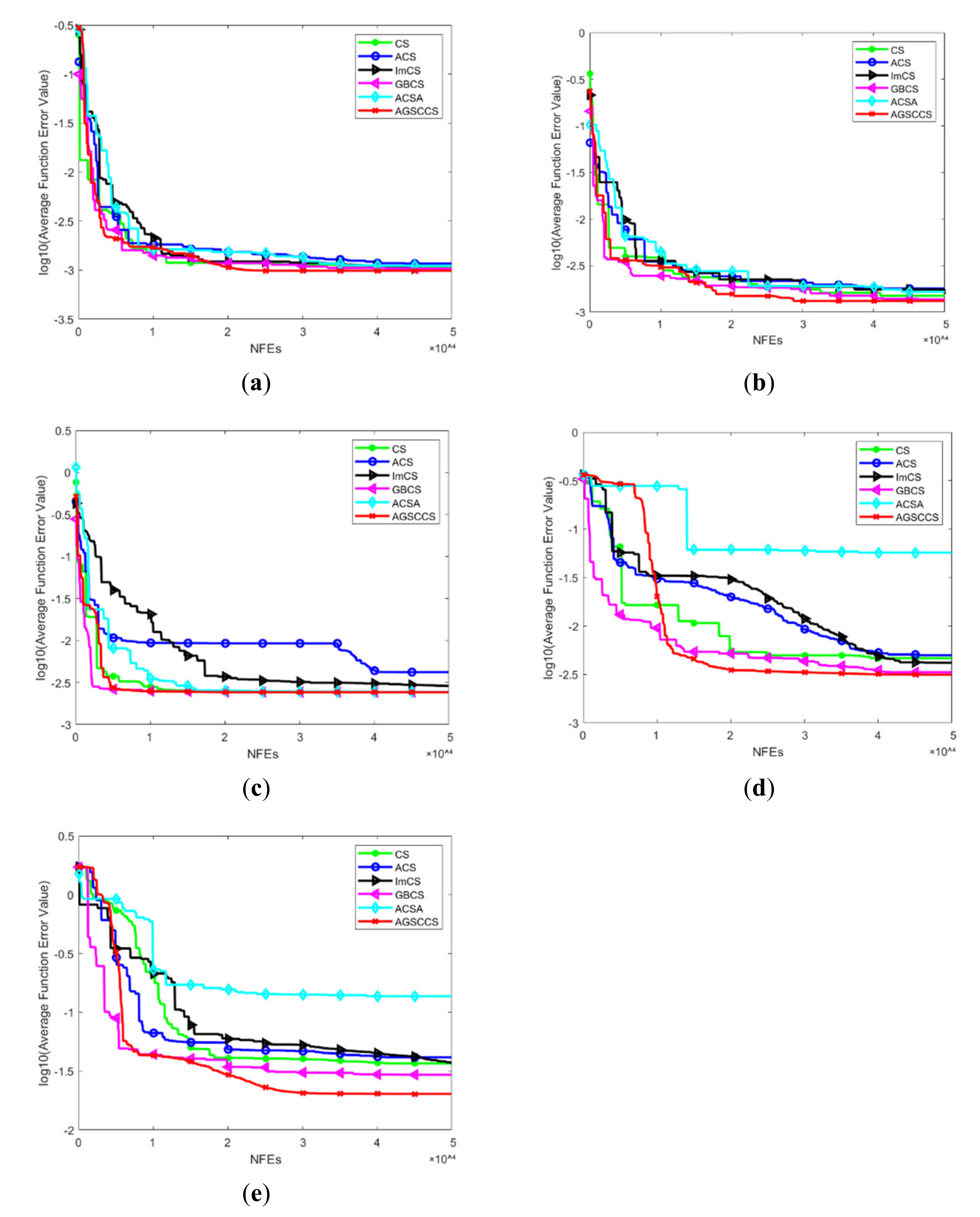
5.2. Results and Analysis

Now, we apply AGSCCS to the PV module parameter optimization problems. To test the performance, it will be compared with ACS, ImCS, GBCS, ACSA, and CS. The specific parameter of the algorithms is set the same. The population size is set to 30 and the function evaluations are set to 50,000. The typical experimental results are stated in

Table 5. Experimental results in PV module.

	CS		ACS		ImCS		GBCS		ACSA		AGSCCS
	Mean	Std	Mean	Std	Mean	Std	Mean	Std	Mean	Std	Mean	Std
SDM	1.08 × 10−3	6.73 × 10−5	1.16 × 10−3	9.57 × 10−5	1.01 × 10−3	4.84 × 10−5	1.04 × 10−3	4.84 × 10−5	1.05 × 10−3	5.92 × 10−5	9.89 × 10−4	1.26 × 10−5
DDM	1.49 × 10−3	2.18 × 10−4	1.80 × 10−3	3.32 × 10−4	1.80 × 10−3	3.09 × 10−4	1.35 × 10−3	2.36 × 10−4	1.69 × 10−3	2.89 × 10−4	1.33 × 10−3	3.28 × 10−4
Photowatt-PWP-201	2.44 × 10−3	7.93 × 10−6	3.00 × 10−3	1.58 × 10−3	2.88 × 10−3	1.12 × 10−3	2.43 × 10−3	1.17 × 10−6	2.45 × 10−3	3.61 × 10−5	2.43 × 10−3	5.32 × 10−6
STM6-40/36	4.66 × 10−3	5.42 × 10−4	4.97 × 10−3	6.27 × 10−4	4.17 × 10−3	5.90 × 10−4	3.35 × 10−3	2.95 × 10−4	5.51 × 10−2	1.03 × 10−1	3.14 × 10−3	5.76 × 10−3
STP6-120/36	3.68 × 10−2	4.91 × 10−3	4.17 × 10−2	6.37 × 10−3	3.74 × 10−2	3.40 × 10−3	2.95 × 10−2	5.19 × 10−3	1.38 × 10−1	3.23 × 10−1	2.02 × 10−2	5.85 × 10−3

.

Table 6. Comparison among different algorithms on SDM PV cell.

Algorithm	${\mathit{I}}_{\mathit{p}\mathit{v}}\left(\mathit{A}\right)$	${\mathit{I}}_{\mathit{s}\mathit{d}}\left(\mathit{A}\right)$	${\mathit{R}}_{\mathit{s}}\left(\Omega \right)$	${\mathit{R}}_{\mathit{p}}\left(\Omega \right)$	$\mathit{\alpha }$	RMSE
CS	0.7607	3.70 × 10−7	0.0358	57.3751	1.4943	1.08 × 10−3
ACS	0.7606	4.36 × 10−7	0.0352	64.9443	1.5110	1.16 × 10−3
ImCS	0.7607	3.54 × 10−7	0.0360	56.7892	1.4905	1.01 × 10−3
GBCS	0.7607	3.64 × 10−7	0.0359	58.2349	1.4928	1.04 × 10−3
ACSA	0.7607	3.57 × 10−7	0.0360	57.2252	1.4910	1.05 × 10−3
AGSCCS	0.7608	3.47 × 10−7	0.0362	54.9470	1.4860	9.89 × 10−4

,

Table 7. Comparison among different algorithms on DDM PV cell.

Algorithm	${\mathit{I}}_{\mathit{p}\mathit{v}}\left(\mathit{A}\right)$	${\mathit{I}}_{\mathit{s}\mathit{d}1}\left(\mathit{A}\right)$	${\mathit{R}}_{\mathit{s}}\left(\Omega \right)$	${\mathit{R}}_{\mathit{p}}\left(\Omega \right)$	$\mathit{\alpha }1$	${\mathit{I}}_{\mathit{s}\mathit{d}2}\left(\mathit{\mu }\mathit{A}\right)$	$\mathit{\alpha }2$	RMSE
CS	0.7606	4.15 × 10−7	0.0350	69.7383	1.6110	2.67 × 10−7	1.6206	1.49 × 10−3
ACS	0.7607	4.88 × 10−7	0.0343	79.6598	1.7060	4.13 × 10−7	1.6896	1.80 × 10−3
ImCS	0.7606	3.65 × 10−7	0.0340	83.2859	1.5794	3.40 × 10−7	1.5826	1.80 × 10−3
GBCS	0.7607	2.77 × 10−7	0.0355	66.2202	1.7133	3.38 × 10−7	1.6354	1.35 × 10−3
ACSA	0.7608	4.24 × 10−7	0.0350	65.8916	1.6702	2.98 × 10−7	1.6187	1.69 × 10−3
AGSCCS	0.7594	2.69 × 10−7	0.0400	79.9490	1.3166	6.61 × 10−8	1.6569	1.33 × 10−3

and

Table 8. Comparison among different algorithms on SMM PV modules.

	Algorithm	${\mathit{I}}_{\mathit{p}\mathit{v}}\left(\mathit{A}\right)$	${\mathit{I}}_{\mathit{s}\mathit{d}}\left(\mathit{A}\right)$	${\mathit{R}}_{\mathit{s}}\left(\Omega \right)$	${\mathit{R}}_{\mathit{p}}\left(\Omega \right)$	$\mathit{\alpha }$	RMSE
Photowatt-PWP-201	CS	1.0302	3.67 × 10−6	1.1959	1048.6362	48.8467	2.44 × 10−3
	ACS	1.0316	3.09 × 10−6	1.2298	928.8406	47.6362	3.00 × 10−3
	ImCS	1.0466	2.68 × 10−6	1.2030	802.3769	46.7762	2.88 × 10−3
	GBCS	1.0304	3.55 × 10−6	1.1992	1007.7580	48.7176	2.43 × 10−3
	ACSA	1.0304	3.53 × 10−6	1.2003	1005.9862	48.6883	2.45 × 10−3
	AGSCCS	1.0305	3.48 × 10−6	1.2013	982.0053	48.6428	2.43 × 10−3
STM6-40/36	CS	1.6552	6.95 × 10−6	0.0002	88.9366	1.6890	4.66 × 10−3
	ACS	1.6556	7.41 × 10−6	0.0002	157.7937	1.6976	4.97 × 10−3
	ImCS	1.6603	5.57 × 10−6	0.0004	30.7576	1.6591	4.17 × 10−3
	GBCS	1.6603	5.43 × 10−6	0.0004	28.2830	1.6562	3.35 × 10−3
	ACSA	1.6468	2.27 × 10−5	0.0060	167.4477	1.8746	5.51 × 10−2
	AGSCCS	1.6633	4.69 × 10−6	0.0034	161.7657	1.7099	3.14 × 10−3
STP6-120/36	CS	7.4960	1.57 × 10−5	0.0036	596.5901	1.4274	3.68 × 10−2
	ACS	7.5113	2.30 × 10−5	0.0032	558.4491	1.4857	4.17 × 10−2
	ImCS	7.5110	2.14 × 10−5	0.0034	1034.5552	1.4677	3.74 × 10−2
	GBCS	7.4909	1.03 × 10−5	0.0038	826.8380	1.3977	2.95 × 10−2
	ACSA	7.4705	4.37 × 10−1	0.0028	349.0301	4.6720	1.38 × 10−1
	AGSCCS	7.4708	3.57 × 10−6	0.0044	418.9095	1.2865	2.02 × 10−2

exhibit the particular value on the SDM PV cells.

Table 5 describes the results of the PV model parameter optimization. Due to the complex nonlinear relationship between the external output characteristics and the internal parameters of the PV modules with the external environment changes, parameter identification of the PV model is a highly complex optimization problem. AGSCCS has the best performance of the six tests. It acquires all the champions in question for the PV model identification compared with the other five algorithms. Especially in SDM, the RMSE of AGSCCS reaches 9.89 × 10⁻⁴, which is much smaller than the rest of the algorithms. It also shows strong competitiveness in other models. It can be said that the comprehensive performance of AGSCCS has been dramatically improved compared with CS. Table 6, Table 7 and Table 8 explicitly exhibit the specific parameter values on the PV model.

Table 6, Table 7 and Table 8 show the parameters associated with identifying the PV model using the AGSCCS algorithm and other five algorithms. As seen from the above table, the optimization results before the algorithm are pretty close. This can be understood as several local optimal near the optimal solution, which will increase the difficulty of convergence of the algorithm. Therefore, CS, ACS, ImCS, GBCS, and ACSA converge only at the local optimal solution. However, AGSCCS can recognize these local optimum solutions and converge to smaller ones, which is sufficient to prove that its exploration ability and exploitation ability have significant advantages over other algorithms.

From Figure 8, AGSCCS shows excellent performance in the PV module parameter setting problems. It always achieves the best results compared with the other five algorithms corresponding with CS. The five problems are nonlinear optimization problems, which are more complex than linear problems. The reason why AGSCCS has the best convergence capacity may owe to the adaptive random step size in the local searching process. It helps search different directions, rather than always search through the best solution’s directions. This measure reduces the risk of falling into the local optimum. Indeed, the increase of accuracy may also give credit to the help of chaotic map initialization, which promotes population diversity in the beginning stage. Moreover, AGSCCS has the fastest convergence speed compared with the other four algorithms. For example, in Figure 8c,d, AGSCCS is close to convergence when the number of function evaluations reaches 30,000, while other algorithms have not reached the convergence value at this time. This is because the SC technique helps accelerate the convergence speed. Compressing the upper and lower bounds reduces the search space without interfering with the direction selection of the algorithm to speed up the convergence speed of the algorithm.

6. Conclusions

In this paper, an Adaptive Guided Spatial Compressive CS (AGSCCS) has been proposed. It mainly aims at improving the section of the local search, which helped enhance the exploitation of AGSCCS. The improvements have been implemented through three steps. The first one was the adjustment of the method of population generation. Due to the heterogeneity of the random number generation method, we adopted a chaotic mapping instead. In this method, chaotic system mapping is used to form the initial solution, which increases the irregularity of the solution arrangement and makes it more like a uniform random distribution. The second one was an adaptive guided scheme of updating location areas. It retained information about the best and worst solution sets in the population and transmitted these to the next generation as clues for finding the ideal solution. The last improvement was a SC technique. It was a novel technique that aimed at quick convergence and better algorithm precision. When taking the SC technique, the population was gathered around the optimal solution, whether the current generation was in local search or global search. Next, it would collect the information of some excellent solutions and transmit the information to the offspring. The three measures above sufficiently considered the balance between exploration and exploitation, giving an outstanding performance. To test the performance of AGSCCS, we tested the algorithm with the other five algorithms (CS, ACS, ImCS, GBCS, and ACSA) on the 2014 CEC benchmark. The experimental results were compared with CS, ACS, ImCS, GBCS, and ACSA. In total, AGSCCS got the best grade. A sensitive examination has been completed to compare the three promotion strategies, which were the most significant contributions. We adopted the controlling variables and compared them. The results revealed that the SC technique has the most significant impact on AGSCCS. In other words, the SC technique made the most contributions to the algorithm. The remaining two strategies were almost equal. However, according to the experimental sensitive test, both of them also contributed to the improvement of the algorithm. At last, we applied AGSCCS into the PV model to verify the feasibility of a practical application. The experiments showed that AGSCCS acquired the best results, which further exemplifies the outstanding performance of the proposed algorithm.

As a metaheuristic algorithm, CS has not been valued for practical applications. As a metaheuristic with few parameters, CS will achieve development in practical applications without question. Next, we will strive to find a competitive CS and apply it into more practical applications in the future. In fact, in Section 5, the photovoltaic model has a deeper level of research value due to its different weather, climate, etc. Using the CS algorithm to study these deeper and more complex models will be a potential direction.

References

1. Sinha, N.; Chakrabarti, R.; Chattopadhyay, P.K. Evolutionary programming techniques for economic load dispatch. IEEE Trans. Evol. Comput. 2003, 7, 83–94. [Google Scholar] [CrossRef]
2. Boushaki, S.I.; Kamel, N.; Bendjeghaba, O. A new quantum chaotic cuckoo search algorithm for data clustering. Expert Syst. Appl. 2018, 96, 358–372. [Google Scholar] [CrossRef]
3. Tejani, G.G.; Pholdee, N.; Bureerat, S.; Prayogo, D.; Gandomi, A.H. Structural optimization using multi-objective modified adaptive symbiotic organisms search. Expert Syst. Appl. 2019, 125, 425–441. [Google Scholar] [CrossRef]
4. Kamoona, A.M.; Patra, J.C. A novel enhanced cuckoo search algorithm for contrast enhancement of gray scale images. Appl. Soft Comput. 2019, 85, 105749. [Google Scholar] [CrossRef]
5. Bérubé, J.-F.; Gendreau, M.; Potvin, J.-Y. An exact-constraint method for biobjective combinatorial optimization problems: Application to the Traveling Salesman Problem with Profits. Eur. J. Oper. Res. 2009, 194, 39–50. [Google Scholar] [CrossRef]
6. Dodu, J.C.; Martin, P.; Merlin, A.; Pouget, J. An optimal formulation and solution of short-range operating problems for a power system with flow constraints. Proc. IEEE 1972, 60, 54–63. [Google Scholar] [CrossRef]
7. Vorontsov, M.A.; Carhart, G.W.; Ricklin, J.C. Adaptive phase-distortion correction based on parallel gradient-descent optimization. Opt. Lett. 1997, 22, 907–909. [Google Scholar] [CrossRef]
8. Parikh, J.; Chattopadhyay, D. A multi-area linear programming approach for analysis of economic operation of the Indian power system. IEEE Trans. Power Syst. 1996, 11, 52–58. [Google Scholar] [CrossRef]
9. Kim, J.S.; Ed Gar, T.F. Optimal scheduling of combined heat and power plants using mixed-integer nonlinear programming. Energy 2014, 77, 675–690. [Google Scholar] [CrossRef]
10. Fan, J.Y.; Zhang, L. Real-time economic dispatch with line flow and emission constraints using quadratic programming. IEEE Trans. Power Syst. 1998, 13, 320–325. [Google Scholar] [CrossRef]
11. Reid, G.F.; Hasdorff, L. Economic Dispatch Using Quadratic Programming. IEEE Trans. Power Appar. Syst. 1973, 6, 2015–2023. [Google Scholar] [CrossRef]
12. Oliveira, P.; Mckee, S.; Coles, C. Lagrangian relaxation and its application to the unit-commitment-economic-dispatch problem. Ima J. Manag. Math. 1992, 4, 261–272. [Google Scholar] [CrossRef]
13. El-Keib, A.A.; Ma, H. Environmentally constrained economic dispatch using the LaGrangian relaxation method. Power Syst. IEEE Trans. 1994, 9, 1723–1729. [Google Scholar] [CrossRef]
14. Aravindhababu, P.; Nayar, K.R. Economic dispatch based on optimal lambda using radial basis function network. Int. J. Electr. Power Energy Syst. 2002, 24, 551–556. [Google Scholar] [CrossRef]
15. Obioma, D.D.; Izuchukwu, A.M. Comparative analysis of techniques for economic dispatch of generated power with modified Lambda-iteration method. In Proceedings of the IEEE International Conference on Emerging & Sustainable Technologies for Power & Ict in A Developing Society, Owerri, Nigeria, 14–16 November 2013; pp. 231–237. [Google Scholar]
16. Mohammadian, M.; Lorestani, A.; Ardehali, M.M. Optimization of Single and Multi-areas Economic Dispatch Problems Based on Evolutionary Particle Swarm Optimization Algorithm. Energy 2018, 161, 710–724. [Google Scholar] [CrossRef]
17. Goldberg, D.E.; Deb, K. A Comparative Analysis of Selection Schemes Used in Genetic Algorithms. Found. Genet. Algorithm. 1991, 1, 69–93. [Google Scholar]
18. Kennedy, J.; Eberhart, R. Particle Swarm Optimization. In Proceedings of the Icnn95-International Conference on Neural Networks, Perth, WA, Australia, 27 November–1 December 1995. [Google Scholar]
19. Yang, X. A new metaheuristic bat-inspired algorithm. In Nature Inspired Cooperative Strategies for Optimization (NICSO); Springer: Berlin/Heidelberg, Germany, 2010. [Google Scholar]
20. Karaboga, D.; Basturk, B. A powerful and efficient algorithm for numerical function optimization: Artificial bee colony (ABC) algorithm. J. Glob. Optim. 2007, 39, 459–471. [Google Scholar] [CrossRef]
21. Sm, A.; Smm, B.; Al, A. Grey Wolf Optimizer. Adv. Eng. Softw. 2014, 69, 46–61. [Google Scholar]
22. Yang, X.S.; Deb, S. Engineering Optimisation by Cuckoo Search. Int. J. Math. Model. Numer. Optim. 2010, 1, 330–343. [Google Scholar] [CrossRef]
23. Ding, J.; Wang, Q.; Zhang, Q.; Ye, Q.; Ma, Y. A Hybrid Particle Swarm Optimization-Cuckoo Search Algorithm and Its Engineering Applications. Math. Probl. Eng. 2019, 2019, 5213759. [Google Scholar] [CrossRef]
24. Mareli, M.; Twala, B. An adaptive Cuckoo search algorithm for optimisation. Appl. Comput. Inform. 2018, 14, 107–115. [Google Scholar] [CrossRef]
25. Naik, M.K.; Panda, R. A novel adaptive cuckoo search algorithm for intrinsic discriminant analysis based face recognition. Appl. Soft Comput. 2016, 38, 661–675. [Google Scholar] [CrossRef]
26. Selvakumar, A.I.; Thanushkodi, K. Optimization using civilized swarm: Solution to economic dispatch with multiple minima. Electr. Power Syst. Res. 2009, 79, 8–16. [Google Scholar] [CrossRef]
27. Hu, P.; Deng, C.; Hui, W.; Wang, W.; Wu, Z. Gaussian bare-bones cuckoo search algorithm. In Proceedings of the the Genetic and Evolutionary Computation Conference Companion, Kyoto, Japan, 15–19 July 2018. [Google Scholar]
28. Walton, S.; Hassan, O.; Morgan, K.; Brown, M.R. Modified cuckoo search: A new gradient free optimisation algorithm. Chaos Solitons Fractals 2011, 44, 710–718. [Google Scholar] [CrossRef]
29. Wang, L.; Zhong, Y.; Yin, Y. Nearest neighbour cuckoo search algorithm with probabilistic mutation. Appl. Soft Comput. 2016, 49, 498–509. [Google Scholar] [CrossRef]
30. Cheng, J.; Wang, L.; Jiang, Q.; Xiong, Y. A novel cuckoo search algorithm with multiple update rules. Appl. Intell. 2018, 48, 4192–4211. [Google Scholar] [CrossRef]
31. Ong, P. Adaptive cuckoo search algorithm for unconstrained optimization. Sci. World J. 2014, 2014, 943403. [Google Scholar] [CrossRef] [PubMed]
32. Kang, T.; Yao, J.; Jin, M.; Yang, S.; Duong, T. A Novel Improved Cuckoo Search Algorithm for Parameter Estimation of Photovoltaic (PV) Models. Energies 2018, 11, 1060. [Google Scholar] [CrossRef] [Green Version]
33. Wang, G.G.; Deb, S.; Gandomi, A.H.; Zhang, Z.; Alavi, A.H. Chaotic cuckoo search. Soft Comput. 2016, 20, 3349–3362. [Google Scholar] [CrossRef]
34. Rakhshani, H.; Rahati, A. Snap-drift cuckoo search: A novel cuckoo search optimization algorithm. Appl. Soft Comput. 2017, 52, 771–794. [Google Scholar] [CrossRef]
35. Shehab, M.; Khader, A.T.; Al-Betar, M.A.; Abualigah, L.M. Hybridizing cuckoo search algorithm with hill climbing for numerical optimization problems. In Proceedings of the 2017 8th International Conference on Information Technology (ICIT), Amman, Jordan, 17–18 May 2017. [Google Scholar]
36. Zhang, Z.; Ding, S.; Jia, W. A hybrid optimization algorithm based on cuckoo search and differential evolution for solving constrained engineering problems. Eng. Appl. Artif. Intell. 2019, 85, 254–268. [Google Scholar] [CrossRef]
37. Pareek, N.K.; Patidar, V.; Sud, K.K. Image encryption using chaotic logistic map. Image Vis. Comput. 2006, 24, 926–934. [Google Scholar] [CrossRef]
38. Mohamed, A.W.; Mohamed, A.K. Adaptive guided differential evolution algorithm with novel mutation for numerical optimization. Int. J. Mach. Learn. Cybern. 2017, 10, 253–277. [Google Scholar] [CrossRef]
39. Aguirre, A.H.; Rionda, S.B.; Coello Coello, C.A.; Lizárraga, G.L.; Montes, E.M. Handling constraints using multiobjective optimization concepts. Int. J. Numer. Methods Eng. 2004, 59, 1989–2017. [Google Scholar] [CrossRef]
40. Wang, Y.; Cai, Z.; Zhou, Y. Accelerating adaptive trade-off model using shrinking space technique for constrained evolutionary optimization. Int. J. Numer. Methods Eng. 2009, 77, 1501–1534. [Google Scholar] [CrossRef]
41. Kaveh, A. Cuckoo Search Optimization; Springer: Cham, Switzerland, 2014; pp. 317–347. [Google Scholar] [CrossRef]
42. Ley, A. The Habits of the Cuckoo. Nature 1896, 53, 223. [Google Scholar] [CrossRef]
43. Humphries, N.E.; Queiroz, N.; Dyer, J.; Pade, N.G.; Musyl, M.K.; Schaefer, K.M.; Fuller, D.W.; Brunnsc Hw Eiler, J.M.; Doyle, T.K.; Houghton, J. Environmental context explains Lévy and Brownian movement patterns of marine predators. Nature 2010, 465, 1066–1069. [Google Scholar] [CrossRef] [Green Version]
44. Wang, R.; Cui, X.; Li, Y. Self-Adaptive adjustment of cuckoo search K-means clustering algorithm. Appl. Res. Comput. 2018, 35, 3593–3597. [Google Scholar]
45. Wilk, G.; Wlodarczyk, Z. Interpretation of the Nonextensivity Parameter q in Some Applications of Tsallis Statistics and Lévy Distributions. Phys. Rev. Lett. 1999, 84, 2770–2773. [Google Scholar] [CrossRef] [Green Version]
46. Nguyen, T.T.; Phung, T.A.; Truong, A.V. A novel method based on adaptive cuckoo search for optimal network reconfiguration and distributed generation allocation in distribution network. Int. J. Electr. Power Energy Syst. 2016, 78, 801–815. [Google Scholar] [CrossRef]
47. Li, X.; Yin, M. Modified cuckoo search algorithm with self adaptive parameter method. Inf. Sci. 2015, 298, 80–97. [Google Scholar] [CrossRef]
48. Naik, M.; Nath, M.R.; Wunnava, A.; Sahany, S.; Panda, R. A new adaptive Cuckoo search algorithm. In Proceedings of the IEEE International Conference on Recent Trends in Information Systems, Kolkata, India, 9–11 July 2015. [Google Scholar]
49. Farswan, P.; Bansal, J.C. Fireworks-inspired biogeography-based optimization. Soft Comput. 2018, 23, 7091–7115. [Google Scholar] [CrossRef]
50. Birx, D.L.; Pipenberg, S.J. Chaotic oscillators and complex mapping feed forward networks (CMFFNs) for signal detection in noisy environments. In Proceedings of the International Joint Conference on Neural Networks, Baltimore, MD, USA, 7–11 June 2002. [Google Scholar]
51. Qi, W. A self-adaptive embedded chaotic particle swarm optimization for parameters selection of Wv-SVM. Expert Syst. Appl. 2011, 38, 184–192. [Google Scholar]
52. Wang, L.; Yin, Y.; Zhong, Y. Cuckoo search with varied scaling factor. Front. Comput. Sci. 2015, 9, 623–635. [Google Scholar] [CrossRef]
53. Das, S.; Mallipeddi, R.; Maity, D. Adaptive evolutionary programming with p-best mutation strategy. Swarm Evol. Comput. 2013, 9, 58–68. [Google Scholar] [CrossRef]
54. Zhang, J.; Sanderson, A.S. JADE: Adaptive Differential Evolution With Optional External Archive. IEEE Trans. Evol. Comput. 2009, 13, 945–958. [Google Scholar] [CrossRef]
55. Deb, K. An efficient constraint handling method for genetic algorithms. Comput. Methods Appl. Mech. Eng. 2000, 186, 311–338. [Google Scholar] [CrossRef]
56. Armani, R.F.; Wright, J.A.; Savic, D.A.; Walters, G.A. Self-Adaptive Fitness Formulation for Evolutionary Constrained Optimization of Water Systems. J. Comput. Civ. Eng. 2005, 19, 212–216. [Google Scholar] [CrossRef]
57. Bo, Y.; Gallagher, M. Experimental results for the special session on real-parameter optimization at CEC 2005: A simple, continuous EDA. In Proceedings of the 2005 IEEE Congress on Evolutionary Computation, Edinburgh, UK, 2–5 September 2005. [Google Scholar]
58. Liang, J.J.; Qu, B.Y.; Suganthan, P.N. Problem Definitions and Evaluation Criteria for the CEC 2014 Special Session and Competition on Single Objective Real-Parameter Numerical Optimization; Technical Report 201311; Computational Intelligence Laboratory, Zhengzhou University: Zhengzhou, China; Nanyang Technological University: Singapore, December 2013. [Google Scholar]
59. Yang, X.; Gong, W. Opposition-based JAYA with population reduction for parameter estimation of photovoltaic solar cells and modules. Appl. Soft Comput. 2021, 104, 107218. [Google Scholar] [CrossRef]
Figure 1. Feeding habits of cuckoos in nature. ①: Mother cuckoos find the best nest within plenty of nests and lay their babies. ②: Baby cuckoos are raised by the hosts. ③: If the hosts find that the cuckoos are not their babies, they will discard them. If the babies are lucky enough not to be found, they will survive ④: If the baby cuckoos are abandoned, mother cuckoos will continue to find the best nest to lay their eggs.
Mathematics 10 00495 g001
Figure 2. 2D plane L é v y flight simulation diagram.
Mathematics 10 00495 g002
Figure 3. Comparison between common initialization and chaotic initialization. (a) Common initialization; (b) Chaotic initialization.
Mathematics 10 00495 g003
Figure 4. Population evolution diagram.
Mathematics 10 00495 g004
Figure 5. Flow chart of AGSCCS.
Mathematics 10 00495 g005
Figure 6. 3D graph of Shifted and Rotated Expanded Griewank’s plus Rosenbrock’s Function.
Mathematics 10 00495 g006
Figure 7. Convergence curve of AGSCCS in CEC2014.
Mathematics 10 00495 g007aMathematics 10 00495 g007bMathematics 10 00495 g007c
Figure 8. Convergence curve of AGSCCS in PV module. (a) SDM; (b) DDM; (c) Photowatt-PWP-201; (d) STM6-40/36; (e) STP6-120/36.
Mathematics 10 00495 g008