Magnetic Field Effects on Thermal Nanofluid Flowing through Vertical Stenotic Artery: Analytical Study

Abstract

The present investigation represents the first complete illustration of nanofluids flow. The effectiveness of wall slip and heat transfer on magnetohydrodynamic nanofluids flow over porous media in vertical stenotic artery with catheter has been analyzed. By considering the long-wavelength with low-Reynolds number approximation, a mathematical solution was derived to velocity, stream function, pressure difference, and temperature. The nanoparticle’s concentration, amplitude ratio, catheter size, and flow rate have been used to extract the pressure difference. This study analyzes the interaction effect of slip and thermal conditions on nanoparticles fluid suspension with a catheter in a vertical stenotic artery with/without the presence of magnetic field and porosity. The results are helpful for understanding the role of the engineering applications of nanofluids in biomedicine and some other applications. The results of this paper reveal that the nanoparticles concentration has little effect on the velocity, and the concentration, slipping, and porosity of the nanoparticles decreases the thermal energy.

1. Introduction

On account of their huge applications in many fields, in this paper we concentrate on the more prominent disciplines of engineering: industrial and biomedical. To improve the thermo-physical properties of the fluids, nanometer particles are injected into them. Several materials can be used to make nanoparticles, such as minerals (gold, silver, ferric, aluminum, copper), nitride ceramics (SiN, AlN), carbide ceramics (SiC, TiC), oxide ceramics (Al₂O₃, CuO), single, double, or many carbon nanotubes (DWCNTs, SWCNTs, MWCNTs), and semiconductors (TiO₂). Basic fluids after injection with these nanoparticles are defined as nanofluids. In general, rigid bodies have major thermo-physical properties comparison with traditional thermo-fluids influence, such as water, oil, and ethylene glycol viscidity, thermoconductance, thermodiffusion, and convective overheat transfer coefficients for these fluids, which are improved by injecting nanoparticles into them. Therefore, the potency of nanofluids in many applications have attracted more and more attention.

In this portion, we will be going to record some applications of nanofluids, such as biomedical applications (antibacterial activity, nanodrug delivery, cancer therapeutic, cryopreservation, nanocryosurgery, molecular imaging and photothermal therapy, ultrasonic image, guided therapy, and MRI imaging). Nanofluids have not been solely applied to the area of biomedicine, but they have been used for distinct bioindustrial engineering areas such as heat transfer intensification (electronic applications, microelectronics, transportation brake and other vehicular nanofluids, manufacture refrigeration implementations, warming houses and reducing defilement, nuclear devices refrigeration, space and defense technologies, pharmaceutical processes, smart fluids, and extraction of geothermal power and other energy sources), mass transfer enhancement, energy apps (power buffering, heliacal sucking), mechanistic apps (friction minimal, magnetohydrodynamic stamping), and other applications (intensification micro-reactors, transportation braking, microbial fuel cell, nanofluids with unique optical properties, nanofluid detergent) [1,2,3,4,5,6,7].

In some instances, the spread of cholesterol in blood vessels blocks the blood, which coagulating inside the cordial artery, deemed as a porous media, [6,8,9]. Chu and Fang [3] considered Newtonian fluid boundary conditions. The effect of slip conditions at the boundary was taken into consideration in the analytical solutions for complex geometries, which have been introduced by Hron et al. [10].

The combined effects between the electrical conductivity of the nanofluids and traditional fluids during the influence of magnetic field and heat transmit overhead convectively heated surfaces is used in engineering and industrial applications. This phenomenon is termed “MHD”, where the magnetic fields can motivate the moving conductive fluid to produce the currents. Due to the induced current, there is a difference in the magnetic field and generating forces on the fluid. Every unit of volume moving through an electric field and magnetic field exposed to a force is known as the Lorentz force [10,11,12]. MHD fluid flows require the augmentation between Navier Stokes equation of fluid dynamics and Maxwell’s equation of electromagnetism. Analytically or numerically, these differential equations have been solved.

The combined impact of the thermic and peristatic effects is exceedingly employed in numerous applications to determine the sensitiveness of thermic viscosity [13,14]. The influence of MHD and wall properties through the peristatic inflow of a Jeffrey nanofluid during duct has been explored [15]. The researchers discussed the mathematical analysis to the influx and the heat transfer. Several significant parameters were examined on the materialistic quantities of the inflow during schemes for Jeffrey and Newtonian fluids. It has been detected that to the Jeffrey fluid, the inflow rate and thermic impact is smaller than that of the Newtonian fluid. In addition, it has been discovered that increasing the concentricity of the nanoparticle leads to a decrease in the velocity and temperature.

For the time being, the impacts of heat transmit together with entropy propagation have been discovered due to the distinguished results by Bejan [16]. Compound integration for entropy propagation and different effects such as friction forces, alchemical reactions, and viscidity lead to more losses of energy in the thermodynamics framework. The entropy propagation performs a renowned pivotal role in various industrial procedures including alchemical vapor sedimentation tools, turbine mechanization, burning, heat exchangers, solar collectors, and refrigeration instruments. Khan and Ali [17] discussed the modern evolutions for modelling and emulation to entropy propagation for dispersed material using self-stimulation. Numerous authors [18,19,20,21] have dedicated their searches for studying entropy propagation for different nonlinear inflow and heat transmit models.

For the time being, nanoscale particles are used in solar energy models because of their thermic advantages. The creation of useful products such as photocatalysts, organic pollutants for minimal concentricity, electrical energy manufacture, and ecological reconquest is due to its powerful oxidizing strength and prolonged stabilization [22,23]. Zeiny et al. [24] presented a crossbred nanofluid founded on solar thermic transmutation competence. Then, they introduced the photothermal transmutation efficiency by Beer’s law. For the time being, most of the researchers focus their search for nanofluids based on nanoparticles with a high thermic conductivity to maximize the heat transmit rate efficiency and to control the heat transmit by using the magnetic field. Shi et al. [25] presented a combination of Fe₃O₄ and TiO₂ nanoparticles to supply with the cleaning and separating circuit. Furthermore, they made a comparison to separate the Fe₃O₄ and TiO₂ nanoparticles at various values of the magnetic field. Prakash et al. [26] have improved the performance of the theoretical micropump for the solar MHD peristatic nanofluid.

In fact, the heat transmit performs a necessary function in acquiring knowledge of the properties of biological tissues. Truly, the mutual analysis around the peristatic and heat transmit are significant for blood thermodynamic characteristics in processes such as oxygenation and hemodialysis, cancer therapy, and hyperthermia [27,28,29]. These joint impacts of heat and mass transmit are important in several types of manufacturing, such as chemical, food, paper, and metallurgical. For further details, see [30,31,32,33,34,35,36,37].

The goal of this paper is to analyze the MHD Newtonian fluid with the effect of heat transfer on nanofluid in an annulus tube with porous medium, considering the slip effects at the wall. This paper is being arranged as follows. Part 1 consists of the modeling problem and the formulation of governing equations with non-dimensional parameters. In part 2, the settling of the problem with the long-wavelength and Low-Reynolds number approximation is presented. The results are then discussed with the previous published data.

2. Materials and Methods

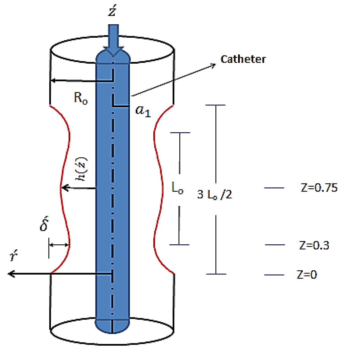
Mathematical Formularization

We impose a viscous nanofluid flow into an asymmetrical circuitous tube with a mean radius R_o. The shear stress is proportional to the velocity gradient, which is known as the Newtonian fluid. Taking the flexibility of the tube walls into consideration, the existence of stenosis makes them fixed. A symmetrical rigid catheter of radius a₁ is implemented. Movement of fluid is caused by the pressure difference at the compliant wall of the tube, as shown in Figure 1.

The stenosis frame can be prescribed as:

$$h(z^{\prime })=\langle R_0-{\delta }^{\prime }{z}^{\prime }\left(11-\frac{94z^{\prime }}{3L_0}+\frac{32}{L_0^2}{z^{\prime }}^2-\frac{32}{3L_0^3}{z^{\prime }}^3\right)\rangle ,$$

(1)

where $L_0$ is the tube length and $z^{\prime }$ is the axial coordinate.

The governing equations to the nanofluid when neglecting the inertia force of the nanoparticles can be considered as [38]:

Mass equation

$$\frac{1}{r^{\prime }}\frac{\partial }{\partial r^{\prime }}\left(r^{\prime }{u}^{\prime }\right)+\frac{\partial }{\partial z^{\prime }}\left(w^{\prime }\right)=0.$$

(2)

Axial momentum

$$\begin{array}{c}{\rho }_{nf}\left[\frac{\partial w^{\prime }}{\partial t^{\prime }}+u^{\prime }\frac{\partial w^{\prime }}{\partial r^{\prime }}+w^{\prime }\frac{\partial w^{\prime }}{\partial z^{\prime }}\right]=-\frac{\partial p^{\prime }}{\partial z^{\prime }}+{\mu }_{nf}\left(\frac{{\partial }^2{w}^{\prime }}{\partial {r^{\prime }}^2}+\frac{1}{r^{\prime }}\frac{\partial w^{\prime }}{\partial r^{\prime }}+\frac{{\partial }^2{w}^{\prime }}{\partial {z^{\prime }}^2}\right)\\ +g{(\rho \gamma )}_{nf}(T^{\prime }-T_1)-{\sigma }_{nf}{\beta }_0^2{w}^{\prime }-\frac{{\mu }_{nf}}{k^{\prime }}{w}^{\prime }.\end{array}$$

(3)

Radial momentum

$${\rho }_{nf}\left[\frac{\partial u^{\prime }}{\partial t^{\prime }}+u^{\prime }\frac{\partial u^{\prime }}{\partial r^{\prime }}+w^{\prime }\frac{\partial u^{\prime }}{\partial z^{\prime }}\right]=-\frac{\partial p^{\prime }}{\partial r^{\prime }}+{\mu }_{nf}(\frac{{\partial }^2{u}^{\prime }}{\partial {r^{\prime }}^2}+\frac{1}{r^{\prime }}\frac{\partial u^{\prime }}{\partial r^{\prime }}-\frac{u^{\prime }}{{r^{\prime }}^2}+\frac{{\partial }^2{u}^{\prime }}{\partial {z^{\prime }}^2}).$$

(4)

The energy equation can be denoted accordingly

$${(\rho c_p)}_{nf}\left[\frac{\partial T^{\prime }}{\partial t^{\prime }}+u^{\prime }\frac{\partial T^{\prime }}{\partial r^{\prime }}+w^{\prime }\frac{\partial T^{\prime }}{\partial z^{\prime }}\right]=K_{nf}\left[\frac{{\partial }^2{T}^{\prime }}{\partial {r^{\prime }}^2}+\frac{1}{r^{\prime }}\frac{\partial T^{\prime }}{\partial r^{\prime }}+\frac{{\partial }^2{T}^{\prime }}{\partial {z^{\prime }}^2}\right]+D+{\sigma }_{nf}\hspace{0.17em}{\beta }_0^2\hspace{0.17em}{w^{\prime }}^2,$$

(5)

where $u^{\prime }$ and $w^{\prime }$ are the velocity components, ${\mu }_{nf}$ is the coefficient of dynamic viscosity of nanofluid, $T^{\prime }$ is the temperature, $c_p$ is the specific heat at constant pressure, and $K_{nf}$ is the thermo-conductivity of nanofluid.

The suggestion of Chu and Fang [3] for the slip boundary conditions on the wall and the catheter can be represented as:

$$w^{\prime }=u_0\pm \mathsf{\Omega }\frac{\partial w^{\prime }}{\partial r^{\prime }},\mathrm{at}{r}^{\prime }=h(z^{\prime }),$$

(6)

$$w^{\prime }=-u_0\pm \mathsf{\Omega }\frac{\partial w^{\prime }}{\partial r^{\prime }}, \mathrm{at}{r}^{\prime }=a_1,$$

(7)

$$T^{\prime }=T_1, \mathrm{at} r^{\prime }=h(z^{\prime }),(\mathrm{isothermal} \mathrm{condition})$$

(8)

$$\frac{\partial T^{\prime }}{\partial r^{\prime }}=0, \mathrm{at} r^{\prime }=a_1, (\mathrm{adiabatic} \mathrm{condition})$$

(9)

where $\mathsf{\Omega }$ is the mean free path and $r^{\prime }$ is the radial coordinate, $\left(w^{\prime }, u^{\prime }\right)$ denotes the fluid phase velocity components along $\left(z^{\prime }, r^{\prime }\right)$ directions, ${\rho }_f$, ${\rho }_s$ are the actual densities of the fluid and nanoparticulate phases, $P^{\prime }$ denotes the pressure, $D$ is the heat source, and $\varnothing$ is the volume fraction of the nanoparticles. An empirical relation for the nanofluid properties can be considered as [2]:

$${\mu }_{nf}=\frac{{\mu }_f}{{(1-\phi )}^{2.5}},{\rho }_{nf}=(1-\phi ){\rho }_f+\phi {\rho }_s,$$

(10)

$${(\rho \gamma )}_{nf}=(1-\phi ){(\rho \gamma )}_f+\phi {(\rho \gamma )}_s,{(\rho c_p)}_{nf}=(1-\phi ){(\rho c_p)}_f+\phi {(\rho c_p)}_s,$$

(11)

$$\frac{K_{nf}}{K_f}=\frac{(K_s+2K_f)-2\phi (K_f-K_s)}{(K_s+2K_f)+\phi (K_f-K_s)},{\sigma }_{nf}=(1-\phi ){\sigma }_f+\phi {\sigma }_s,$$

(12)

where, ${\sigma }_f, {\sigma }_s, {\sigma }_{nf}, K_f, K_s, K_{nf}$ are the electrical and thermal conductivity of fluid, nanoparticles, and nanofluid, respectively.

Setting the next nondimensional variables:

$$z=\frac{z^{\prime }}{L_0},r=\frac{r^{\prime }}{R_0},u=\frac{L_0{u}^{\prime }}{{\delta }^{\prime }\hspace{0.17em}{u}_0},w=\frac{w^{\prime }}{u_0},Re=\frac{{\rho }_f{u}_0{L}_0}{{\mu }_f},\delta =\frac{{\delta }^{\prime }}{R_0},$$

$$p=\frac{R_0{}^2}{{\mu }_f{u}_0{L}_0}{p}^{\prime },\epsilon =\frac{R_0}{L_0},t=\frac{u_0{t}^{\prime }}{R_0},\theta =\frac{T^{\prime }-T_1}{T_0-T_1},Ha=\sqrt{\frac{{\sigma }_f}{{\mu }_f}}{\beta }_0{R}_0,$$

$$k=\frac{k^{\prime }}{R_0^2},Gr=\frac{g{(\rho \gamma )}_f{R}_0{}^2(T_0-T_1)}{u_0{\mu }_f},Br=\frac{{\mu }_f{u}_0^2}{K_f(T_0-T_1)},Kn=\frac{\mathsf{\Omega }}{R_0}$$

where $Kn$ is the Knudsen number, $\theta$ is the nondimensional temperature, $k$ is the nondimensional permeability parameter, $Ha$ is Hartman number, $Re$ is the Reynolds number of nanofluid, $Gr$ is the Grashof number, $Br$ is the Brinkman number, $T_1$ is the inner wall temperature, and $T_0$ ambient air temperature.

The governing Equations (2)–(9) with the non-dimensional parameters can be changed to the following equations:

$$\frac{1}{r}\frac{\partial }{\partial r}\left(ru\right)+\frac{\partial }{\partial z}\left(w\right)=0$$

(13)

$$\begin{array}{c}\frac{{\rho }_{nf}}{{\rho }_f}\mathit{Re}\left[\epsilon \frac{\partial w}{\partial t}+{\epsilon }^2\delta \hspace{0.17em}u\frac{\partial w}{\partial r}+{\epsilon }^{2}w\frac{\partial w}{\partial z}\right]=-\frac{\partial p}{\partial z}-H{a}^2\hspace{0.17em}\left(1-\phi +\frac{{\sigma }_s}{{\sigma }_f}\right)w\\ -\frac{1}{K{\left(1-\phi \right)}^{2.5}}w+\frac{{\mu }_{nf}}{{\mu }_f}\left(\frac{{\partial }^{2}w}{\partial r^2}+\frac{1}{r}\frac{\partial w}{\partial r}+{\epsilon }^2\frac{{\partial }^{2}w}{\partial z^2}\right)+\frac{{(\rho \gamma )}_{nf}}{{(\rho \gamma )}_f}Gr\theta \end{array}$$

(14)

$$\frac{{\rho }_{nf}}{{\rho }_f}Re\left[\frac{u_0}{L_0^2}\delta \frac{\partial u}{\partial t}+{\epsilon }^4{\delta }^2\hspace{0.17em}u\frac{\partial u}{\partial r}+{\epsilon }^3\delta \hspace{0.17em}w\frac{\partial u}{\partial z}\right]=-\frac{\partial p}{\partial r}+\frac{{\mu }_{nf}}{{\mu }_f}(\delta \frac{{\partial }^{2}u}{\partial r^2}+\frac{\delta }{r}\frac{\partial u}{\partial r}-\delta \frac{u}{r^2}+\epsilon \frac{{\partial }^{2}u}{\partial z^2})$$

(15)

$$\begin{array}{c}\mathit{Re}\frac{{\mu }_f{(\rho c_p)}_{nf}}{{\rho }_f{K}_{nf}}\epsilon \left[\frac{\partial \theta }{\partial t}+\epsilon \delta \hspace{0.17em}u\frac{\partial \theta }{\partial r}+\epsilon w\frac{\partial \theta }{\partial z}\right]=\left(\frac{{\partial }^2\theta }{\partial r^2}+\frac{1}{r}\frac{\partial \theta }{\partial r}+{\epsilon }^2\frac{{\partial }^2\theta }{\partial z^2}\right)+S\frac{K_f}{K_{nf}}\\ \hspace{0.17em}+H{a}^2\hspace{0.17em}\hspace{0.17em}\hspace{0.17em}\frac{K_f}{K_{nf}}\hspace{0.17em}\hspace{0.17em}Br\hspace{0.17em}\hspace{0.17em}\left(1-\phi +\phi \frac{{\sigma }_s}{{\sigma }_f}\right)w^2\end{array}$$

(16)

The dimensionless stenosis frame equation becomes:

$$h(z)=\langle 1-\delta z\left(11-\frac{94z}{3L_0}+\frac{32}{L_0^2}{z}^2-\frac{32}{3L_0^3}{z}^3\right)\rangle .$$

(17)

Solution Procedure

Employing the long wavelength approach $\left(\delta \ll 1, \epsilon \approx 0\left(1\right)\right)$ used in Shapiro et al. [39], the set equations which describe the flow through the stenosis shape can be expressed as:

Redial momentum equation

$$\frac{\partial p}{\partial r}=0\mathrm{thus} \frac{dp}{dz}=\frac{\partial p}{\partial z}.$$

(18)

Axial momentum equation

$${(1-\phi )}^{2.5}\hspace{0.17em}\hspace{0.17em}\frac{dp}{dz}=\left[\frac{{\partial }^{2}w}{\partial r^2}+\frac{1}{r}\frac{\partial w}{\partial r}\right]-\left(H{a}^2\hspace{0.17em}{\left(1-\phi \right)}^{2.5}\left(1-\phi +\phi \frac{{\sigma }_s}{{\sigma }_f}\right)+\frac{1}{k}\right)w+{\left(1-\phi \right)}^{2.5}\hspace{0.17em}\hspace{0.17em}\frac{{(\rho \gamma )}_{nf}}{{(\rho \gamma )}_f}\hspace{0.17em}Gr\hspace{0.17em}\theta .$$

(19)

Energy equation

$$\left(\frac{{\partial }^2\theta }{\partial r^2}+\frac{1}{r}\frac{\partial \theta }{\partial r}\right)+S\frac{K_f}{K_{nf}}+H{a}^2\left(1-\phi +\phi \frac{{\sigma }_s}{{\sigma }_f}\right)\frac{K_f}{K_{nf}}Br\hspace{0.17em}{w}^2=0.$$

(20)

The non-dimensional slip velocity and temperature conditions are:

$$w=1\pm Kn\frac{\partial w}{\partial r}\mathrm{at} r=h(z),$$

(21)

$$w=-1\pm Kn\frac{\partial w}{\partial r}\mathrm{at} r=\mathrm{J},$$

(22)

$$\theta =0,.\mathrm{at} r=h(z),$$

(23)

$$\frac{\partial \theta }{\partial r}=0,.\mathrm{at} r=\mathrm{J},$$

(24)

The dimensionless parameters in the previous equations are: $\mathrm{J}=$ catheter size $\left(\mathrm{J}=\frac{a_1}{R_0}\right)$,

The expression of the velocity $w$ can be obtained from the solution of the Equation (19), by introducing the boundary conditions (21) and (22):

$$w=C_{1}b{r}_1+C_{2}b{r}_2-\frac{{(1-\phi )}^{2.5}\frac{dp}{dz}-A}{B}.$$

(25)

The stream function can be got from the relationship of the velocity accordingly:

$$w=\frac{1}{r}\frac{\partial \psi }{\partial r},$$

(26)

$$\psi (z,r)={\displaystyle \mathsf{\int }r\hspace{0.17em}w\hspace{0.17em}\hspace{0.17em}dr},$$

(27)

$$\begin{array}{c}\psi (z,r)=\frac{C_1}{\sqrt{B}}\left(r\hspace{0.17em}{I}_1(\sqrt{B}r)-\mathrm{J}{I}_1(\sqrt{B}\mathrm{J})\right)+\frac{C_2}{\sqrt{B}}\left(r\hspace{0.17em}{K}_1(\sqrt{B}r)-\mathrm{J}{K}_1(\sqrt{B}\mathrm{J})\right)\\ +\frac{\left({(1-\phi )}^{2.5}\frac{dp}{dz}-A\right)}{2B}\left({\mathrm{J}}^2-r^2\right),\end{array}$$

(28)

where $C_1$, $C_2$ are

$$\begin{array}{l}{C}_1=\frac{(b{\mathrm{J}}_2-Kn\hspace{0.17em}{q}_4)\left(1+\frac{1}{B}\left({(1-\phi )}^{2.5}\frac{dp}{dz}-A\right)\right)-(b{h}_2-Kn\hspace{0.17em}{q}_2)\left(-1+\frac{1}{B}\left({(1-\phi )}^{2.5}\frac{dp}{dz}-A\right)\right)}{(b{h}_1-Kn\hspace{0.17em}{q}_1)(b{\mathrm{J}}_2-Kn\hspace{0.17em}{q}_4)-(b{h}_2-Kn\hspace{0.17em}{q}_2)(b{\mathrm{J}}_1-Kn\hspace{0.17em}{q}_3)},\\ \end{array}$$

$$\begin{array}{l}{C}_2=\frac{(b{h}_1-Kn\hspace{0.17em}{q}_1)\left(-1+\frac{1}{B}\left({(1-\phi )}^{2.5}\frac{dp}{dz}-A\right)\right)-(b{\mathrm{J}}_1-Kn\hspace{0.17em}{q}_3)\left(1+\frac{1}{B}\left({(1-\phi )}^{2.5}\frac{dp}{dz}-A\right)\right)}{(b{h}_1-Kn\hspace{0.17em}{q}_1)(b{\mathrm{J}}_2-Kn\hspace{0.17em}{q}_4)-(b{h}_2-Kn\hspace{0.17em}{q}_2)(b{\mathrm{J}}_1-Kn\hspace{0.17em}{q}_3)},\\ \end{array}$$

From which,

$$b{r}_1=I_0(\sqrt{B}r)=1+\frac{B{r}^2}{4}+\frac{B^2{r}^4}{64}+\dots \dots ,$$

$$b{r}_2=K_0(\sqrt{B}r)=-\ln (\frac{\sqrt{B}r}{2})-\frac{B{r}^2\ln (\frac{\sqrt{B}r}{2})}{4}+\frac{(2-2\gamma )B{r}^2}{8}-\gamma +\dots \dots ,$$

$$b{h}_1=I_0(\sqrt{B}h),\hspace{0.17em}\hspace{0.17em}\hspace{0.17em}\hspace{0.17em}\hspace{0.17em}b{h}_2=K_0(\sqrt{B}h),\hspace{0.17em}\hspace{0.17em}\hspace{0.17em}\hspace{0.17em}\hspace{0.17em}\hspace{0.17em}b{\mathrm{J}}_1=I_0(\sqrt{B}\mathrm{J}),\hspace{0.17em}\hspace{0.17em}\hspace{0.17em}\hspace{0.17em}\hspace{0.17em}\hspace{0.17em}b{\mathrm{J}}_2=K_0(\sqrt{B}\mathrm{J}),$$

$$q_1=\frac{\partial b{h}_1}{\partial h},q_2=\frac{\partial b{h}_2}{\partial h},q_3=\frac{\partial b{\mathrm{J}}_1}{\partial \mathrm{J}},q_4=\frac{\partial b{\mathrm{J}}_2}{\partial \mathrm{J}},B=H{a}^2{(1-\phi )}^{2.5}\left(1-\phi +\phi \frac{{\sigma }_s}{{\sigma }_f}\right)+\frac{1}{k},$$

$$b{h}_{\hspace{0.17em}11}={\displaystyle \mathsf{\int }h\hspace{0.17em}b{h}_{\hspace{0.17em}1}\hspace{0.17em}dh},\hspace{0.17em}\hspace{0.17em}\hspace{0.17em}b{h}_{\hspace{0.17em}22}={\displaystyle \mathsf{\int }h\hspace{0.17em}b{h}_{\hspace{0.17em}2}\hspace{0.17em}dh},\hspace{0.17em}\hspace{0.17em}\hspace{0.17em}b{\mathrm{J}}_{\hspace{0.17em}11}=\hspace{0.17em}{\displaystyle \mathsf{\int }\mathrm{J}\hspace{0.17em}b{\mathrm{J}}_1\hspace{0.17em}d\mathrm{J}},\hspace{0.17em}\hspace{0.17em}\hspace{0.17em}b{\mathrm{J}}_{\hspace{0.17em}22}={\displaystyle \mathsf{\int }\mathrm{J}\hspace{0.17em}b{\mathrm{J}}_{\hspace{0.17em}2}\hspace{0.17em}d\mathrm{J}},$$

$$A={(1-\phi )}^{2.5}\left(1-\phi +\phi \frac{{(\rho \gamma )}_s}{{(\rho \gamma )}_f}\right)Gr(-0.04712557038 {\mathrm{J}}^2\ln (h)+0.02356278519h^2).$$

Here, $I_0$ is the modified Bessel function of the first kind with zero order.

$K_0$ is the modified Bessel function of the second kind with zero order.

Then, one can now obtain the pressure difference from the flow rate as;

$$Q={\displaystyle \underset{\mathrm{J}}{\overset{h}{\mathsf{\int }}}r\hspace{0.17em}w(z,r)\hspace{0.17em}dr},$$

(29)

$$\frac{dp}{dz}=\frac{\partial p}{\partial z}=\frac{\left(\begin{array}{l}Q-\frac{(b{\mathrm{J}}_2-Kn\hspace{0.17em}{q}_4)+(b{h}_2-Kn\hspace{0.17em}{q}_2)}{((b{h}_1-Kn\hspace{0.17em}{q}_1)\hspace{0.17em}(b{\mathrm{J}}_2-Kn\hspace{0.17em}{q}_4)-(b{\mathrm{J}}_1-Kn\hspace{0.17em}{q}_3)\hspace{0.17em}(b{h}_2-Kn\hspace{0.17em}{q}_2))}b{h}_{11}\\ +\frac{((b{\mathrm{J}}_2-Kn\hspace{0.17em}{q}_4)-(b{h}_2-Kn\hspace{0.17em}{q}_2))A}{B((b{h}_1-Kn\hspace{0.17em}{q}_1)\hspace{0.17em}(b{\mathrm{J}}_2-Kn\hspace{0.17em}{q}_4)-(b{\mathrm{J}}_1-Kn\hspace{0.17em}{q}_3)\hspace{0.17em}(b{h}_2-Kn\hspace{0.17em}{q}_2))}b{h}_{11}\\ +\frac{((b{h}_1-Kn\hspace{0.17em}{q}_1)-(b{\mathrm{J}}_1-Kn\hspace{0.17em}{q}_3)}{((b{h}_1-Kn\hspace{0.17em}{q}_1)\hspace{0.17em}(b{\mathrm{J}}_2-Kn\hspace{0.17em}{q}_4)-(b{\mathrm{J}}_1-Kn\hspace{0.17em}{q}_3)\hspace{0.17em}(b{h}_2-Kn\hspace{0.17em}{q}_2))}b{h}_{22}\\ +\frac{((b{h}_1-Kn\hspace{0.17em}{q}_1)-(b{\mathrm{J}}_1-Kn\hspace{0.17em}{q}_3))A}{B((b{h}_1-Kn\hspace{0.17em}{q}_1)\hspace{0.17em}(b{\mathrm{J}}_2-Kn\hspace{0.17em}{q}_4)-(b{\mathrm{J}}_1-Kn\hspace{0.17em}{q}_3)\hspace{0.17em}(b{h}_2-Kn\hspace{0.17em}{q}_2))}b{h}_{22}-\frac{A{h}^2}{2B}\\ +\frac{((b{\mathrm{J}}_2-Kn\hspace{0.17em}{q}_4)+(b{h}_2-Kn\hspace{0.17em}{q}_2))A}{((b{h}_1-Kn\hspace{0.17em}{q}_1)\hspace{0.17em}(b{\mathrm{J}}_2-Kn\hspace{0.17em}{q}_4)-(b{\mathrm{J}}_1-Kn\hspace{0.17em}{q}_3)\hspace{0.17em}(b{h}_2-Kn\hspace{0.17em}{q}_2))}b{\mathrm{J}}_{11}\\ -\frac{((b{\mathrm{J}}_2-Kn\hspace{0.17em}{q}_4)-(b{h}_2-Kn\hspace{0.17em}{q}_2))A}{B((b{h}_1-Kn\hspace{0.17em}{q}_1)\hspace{0.17em}(b{\mathrm{J}}_2-Kn\hspace{0.17em}{q}_4)-(b{\mathrm{J}}_1-Kn\hspace{0.17em}{q}_3)\hspace{0.17em}(b{h}_2-Kn\hspace{0.17em}{q}_2))}b{\mathrm{J}}_{11}\\ -\frac{(b{h}_1-Kn\hspace{0.17em}{q}_1)+(b{\mathrm{J}}_1-Kn\hspace{0.17em}{q}_3)}{((b{h}_1-Kn\hspace{0.17em}{q}_1)\hspace{0.17em}(b{\mathrm{J}}_2-Kn\hspace{0.17em}{q}_4)-(b{\mathrm{J}}_1-Kn\hspace{0.17em}{q}_3)\hspace{0.17em}(b{h}_2-Kn\hspace{0.17em}{q}_2))}b{\mathrm{J}}_{22}\\ -\frac{((b{h}_1-Kn\hspace{0.17em}{q}_1)-(b{\mathrm{J}}_1-Kn\hspace{0.17em}{q}_3))A}{B((b{h}_1-Kn\hspace{0.17em}{q}_1)\hspace{0.17em}(b{\mathrm{J}}_2-Kn\hspace{0.17em}{q}_4)-(b{\mathrm{J}}_1-Kn\hspace{0.17em}{q}_3)\hspace{0.17em}(b{h}_2-Kn\hspace{0.17em}{q}_2))}b{\mathrm{J}}_{22}+\frac{A{\mathrm{J}}^2}{2B}\end{array}\right)}{{(1-\phi )}^{2.5}\left(\begin{array}{c}\frac{(b{\mathrm{J}}_2-Kn\hspace{0.17em}{q}_4)-(b{h}_2-Kn\hspace{0.17em}{q}_2)}{B((b{h}_1-Kn\hspace{0.17em}{q}_1)\hspace{0.17em}(b{\mathrm{J}}_2-Kn\hspace{0.17em}{q}_4)-(b{\mathrm{J}}_1-Kn\hspace{0.17em}{q}_3)\hspace{0.17em}(b{h}_2-Kn\hspace{0.17em}{q}_2))}b{h}_{11}\\ +\frac{((b{h}_1-Kn\hspace{0.17em}{q}_1)-(b{\mathrm{J}}_1-Kn\hspace{0.17em}{q}_3))}{B((b{h}_1-Kn\hspace{0.17em}{q}_1)\hspace{0.17em}(b{\mathrm{J}}_2-Kn\hspace{0.17em}{q}_4)-(b{\mathrm{J}}_1-Kn\hspace{0.17em}{q}_3)\hspace{0.17em}(b{h}_2-Kn\hspace{0.17em}{q}_2))}b{h}_{22}\\ -\frac{h^2}{2B}-\frac{((b{\mathrm{J}}_2-Kn\hspace{0.17em}{q}_4)-(b{h}_2-Kn\hspace{0.17em}{q}_2))}{B((b{h}_1-Kn\hspace{0.17em}{q}_1)\hspace{0.17em}(b{\mathrm{J}}_2-Kn\hspace{0.17em}{q}_4)-(b{\mathrm{J}}_1-Kn\hspace{0.17em}{q}_3)\hspace{0.17em}(b{h}_2-Kn\hspace{0.17em}{q}_2))}b{\mathrm{J}}_{11}\\ -\frac{((b{h}_1-Kn\hspace{0.17em}{q}_1)-(b{\mathrm{J}}_1-Kn\hspace{0.17em}{q}_3))}{B((b{h}_1-Kn\hspace{0.17em}{q}_1)\hspace{0.17em}(b{\mathrm{J}}_2-Kn\hspace{0.17em}{q}_4)-(b{\mathrm{J}}_1-Kn\hspace{0.17em}{q}_3)\hspace{0.17em}(b{h}_2-Kn\hspace{0.17em}{q}_2))}b{\mathrm{J}}_{22}+\frac{{\mathrm{J}}^2}{2B}\end{array}\right)}$$

$$\mathsf{\Delta }p=-{\displaystyle \underset{0}{\overset{l}{\mathsf{\int }}}\frac{dp}{dz}\hspace{0.17em}dz}.$$

(30)

The expression of the temperature $\theta$ obtained as the solution of Equation (20), subjected to temperature conditions (23) and (24) is:

$$\theta =L_1+L_2\ln (r)+{\varpi }_1+{\varpi }_{21}+{\varpi }_{22}+{\varpi }_{23}+{\varpi }_{24}+{\varpi }_{25}+{\varpi }_{26},$$

(31)

$$L_1=-L_2\hspace{0.17em}\ln (h)-({\zeta }_1+{\zeta }_{21}+{\zeta }_{22}+{\zeta }_{23}+{\zeta }_{24}+{\zeta }_{25}+{\zeta }_{26}),$$

(32)

$$L_2=-\mathrm{J}({\vartheta }_1+{\vartheta }_{21}+{\vartheta }_{22}+{\vartheta }_{23}+{\vartheta }_{24}+{\vartheta }_{25}+{\vartheta }_{26}),$$

(33)

where:

$$\begin{array}{l}{\zeta }_i=\theta p{h}_i=\hspace{0.17em}\hspace{0.17em}\hspace{0.17em}{\theta p{r}_i|}_{r=h}\hspace{0.17em}\hspace{0.17em},\hspace{0.17em}\hspace{0.17em}\hspace{0.17em}{\vartheta }_i={\frac{\partial \theta p{r}_i}{\partial r}|}_{r=\mathrm{J}}\hspace{0.17em},\hspace{0.17em}\hspace{0.17em}where\hspace{0.17em}\hspace{0.17em}i=1,21,22,23,24,25,26\\ {\varpi }_1=\theta p{r}_1=-\frac{S{r}^2{K}_f}{4K_{nf}},\\ {\varpi }_{21}=\theta p{r}_{21}=-E{C}_1^2\left(\frac{r^2}{4}+\frac{B^2{r}^6}{576}+\frac{B{r}^4}{32}+\frac{B^4{r}^{10}}{\mathrm{409,600}}+\frac{B^2{r}^6}{1152}+\frac{B^3{r}^8}{8192}\right)\end{array}$$

$$\begin{array}{l}{\varpi }_{22}=\theta p{r}_{22}=-E{C}_2^2\{{\left(\ln \left(\frac{\sqrt{B}}{2}\right)\right)}^2\left(\frac{r^2}{4}+\frac{B^2{r}^6}{576}+\frac{B\hspace{0.17em}{r}^4}{32}\right)+2\ln \left(\frac{\sqrt{B}}{2}\right)(\frac{r^2}{4}\left(\ln (r)-1\right)\\ +\frac{B^2{r}^6}{576}\left(\ln (r)-\frac{1}{3}\right)+\frac{B\hspace{0.17em}{r}^4}{32}\left(\ln (r)-\frac{1}{2}\right))+\frac{r^2}{4}\left({\left(\ln \left(r\right)\right)}^2-2\ln (r)+\frac{3}{2}\right)\\ +\frac{B^2{r}^6}{576}\left({\left(\ln \left(r\right)\right)}^2-\frac{2}{3}\ln (r)+\frac{1}{6}\right)+\frac{B\hspace{0.17em}{r}^4}{32}\left({\left(\ln \left(r\right)\right)}^2-\ln (r)+\frac{6}{16}\right)\}\end{array}$$

$$\begin{array}{c}{\varpi }_{23}=\theta p{r}_{23}=-2E\hspace{0.17em}{C}_1\hspace{0.17em}{C}_2\{\ln \left(\frac{\sqrt{B}}{2}\right)\hspace{0.17em}\hspace{0.17em}\left(-\frac{r^2}{4}-\frac{B^2{r}^6}{576}-\frac{B\hspace{0.17em}{r}^4}{32}-\frac{B^2{r}^6}{2304}-\frac{B^3{r}^8}{16384}\right)\\ -\left(\frac{r^2}{4}\left(\ln (r)-1\right)+\frac{B^2{r}^6}{576}\left(\ln (r)-\frac{1}{3}\right)+\frac{B\hspace{0.17em}{r}^4}{32}\left(\ln (r)-\frac{1}{2}\right)\right)\\ -\frac{B^2{r}^6}{2304}\left(\ln (r)-\frac{1}{3}\right)-\frac{B^3{r}^8}{16384}\left(\ln (r)-\frac{1}{4}\right)\}\end{array}$$

$${\varpi }_{24}=\theta p{r}_{24}=2mE{C}_1\left(\frac{r^2}{4}+\frac{B^2{r}^6}{2304}+\frac{B\hspace{0.17em}{r}^4}{64}\right),\hspace{0.17em}$$

$${\varpi }_{25}=\theta p{r}_{25}=-2mE{C}_2\left(\frac{r^2}{4}\ln \left(\frac{\sqrt{B}}{2}\right)+\frac{r^2}{4}(\ln (r)-1)+\frac{B\hspace{0.17em}{r}^4}{64}\left(\ln \left(\frac{\sqrt{B}}{2}\right)+(\ln (r)-\frac{1}{2})\right)\right)$$

$${\varpi }_{26}=\theta p{r}_{26}=-\frac{m^{2}E{r}^2}{4}$$

$$m=\frac{\left({(1-\phi )}^{2.5}\frac{dp}{dz}-A\right)}{B},\hspace{0.17em}\hspace{0.17em}\hspace{0.17em}E=H{a}^2\left(1-\phi +\phi \frac{{\sigma }_s}{{\sigma }_f}\right)\frac{K_f}{K_{nf}}Br$$

3. Results

3.1. Validation of the Problem

Equations (25) and (33) represent the same formula as by Mekheimer [40], when neglecting the effect of nanoparticles on electrical conductivity, porosity, slip condition on the flow behavior, and the effect of magnetic field on the energy equation, Figure 2.

3.2. Numerical Analysis and Discussion

The influence of several parameters containing the nanoparticles concentricity, $\phi$, the catheter size, $\mathrm{J}$, and the amplitude ratio of stenosis, $\delta$ will be shown. The parameter values are chosen as: $R_0$ (tube radius) = 12.5 mm; $\phi$ = 0, 0.02, 0.04, and 0.05; $\delta$ = 0, 0.02 and 0.04; $\mathrm{J}$ = 0, 0.1, 0.2 and 0.3 [38]; and Q = 0.1, 0.2, and 0.3. On the other hand, the results of the thermal study have been achieved through various flow rate (Q = 0.1, 0.2, 0.3), catheter size ($\mathrm{J}$ = 0.1, 0.2, 0.3), stenosis amplitude ratio ($\delta$ = 0, 0.02, 0.04), and nanoparticles concentration ($\phi$ = 0, 0.02, 0.04).

Figure 3 displays the axial flow velocity at various positions. At z = 0.3, the reduced flow area causes the velocity to increase, while at z = 0 the velocity decreases because of the growing cross section.

Figure 4 describes the velocity distributions for different flow rates, the velocity profiles show an increase of the centric velocity for the inflow rate near the wall but a decrease near the catheter because of the opposite direction of the catheter movement. The concentration effect of the nanoparticles on the velocity distribution is seen in Figure 5.

Table 1. Velocity with different nanoparticles concentrations at (Kn = 0, S = 0.1, k = 0.1, Ha = 10⁻⁵, J = 0.2, Q = 0.2, δ = 0.02).

Radial (r)	Velocity (w)
0.2	−1	−1	−1
0.3	−0.6028394149	−0.6028389455	−0.6028384998
0.4	−0.3424592848	−0.3424587957	−0.3424583314
0.5	−0.1391933897	−0.1391930735	−0.1391927738
0.6	0.0469001562	0.0469002316	0.0469003025
0.7	0.2419012707	0.2419011186	0.2419009731
0.8	0.4672595276	0.4672592396	0.4672589629
0.9	0.7443480614	0.7443478223	0.7443475934
1	1	1	1

describes the small effect of nanoparticles concentration on the velocity distribution of the nanofluid.

Figure 6 investigates the influence of slip condition on fluid velocity profiles with a different Knudsen number. It is noticed that the near-wall velocity is enhanced due to the Knudsen number, while the Knudsen number at the catheter decreases the near-wall velocity, because the catheter moves in the opposite direction of the fluid at the inlet.

Figure 7 shows the fluid velocity with MHD at various magnetic fields. It was noted that the Hartman number within the tube wall increases the velocity at the wall, whilst the catheter velocity is decreased close to the wall.

Figure 8 shows that the velocity distributions are affected by the permeability parameter and that the porous media increases the velocity. The velocity increases with the catheter, as shown in Figure 9.

Figure 10 represents the relation between the amplitude ratio (δ) and the velocity distribution. The velocity decreases when the amplitude ratio (δ) increases. If the movement of the catheter is the same motion direction as the nanofluid at the wall of the artery stenosis, there is a symmetrical velocity distribution (see Figure 11). The influence of different values of the flow rate on the stream function is shown in Figure 12. The effect of the Knudsen number, porosity, and magnetic field is shown in Figure 13, Figure 14 and Figure 15. It is observed that the streamlines are crowded with the flow rate.

Figure 16 shows the temperature gradient versus the locations. The flux rate has a significant role in promoting the temperature, in which the thermic energy increases with increasing flowing rate (see Figure 17). The temperature (θ) decreases with the concentration of nanoparticles (φ), as seen in Figure 18, with the presence of Knudsen number.

The temperature is strongly affected by the magnetic field (Ha), as shown in Figure 19, in which the temperature increases when increasing the magnetic field. With slipping, the presence of the catheter decreases the temperature (see Figure 20). Figure 21 shows the effect of stenosis amplitude ratio (δ) on the temperature, in which the temperature decreases when (δ) increases.

The presence of amplitude ratio, flow rate, nanoparticles concentration, magnetic field, and Knudsen number increase the pressure difference, unlike the presence of catheter and gravity (see Figure 22, Figure 23, Figure 24, Figure 25, Figure 26, Figure 27, Figure 28 and Figure 29).

4. Conclusions

This paper analyzes the interaction effect of slip and thermal conditions on nanoparticle fluid suspension with a catheter in vertical stenotic artery with/without the presence of a magnetic field through porous media. The analytical method of settling has been investigated and used for excerption, the velocity and temperature of the fluid for a regular tube with a long wavelength, and low Reynolds number approximation.

From the present study, the following points are noticed:

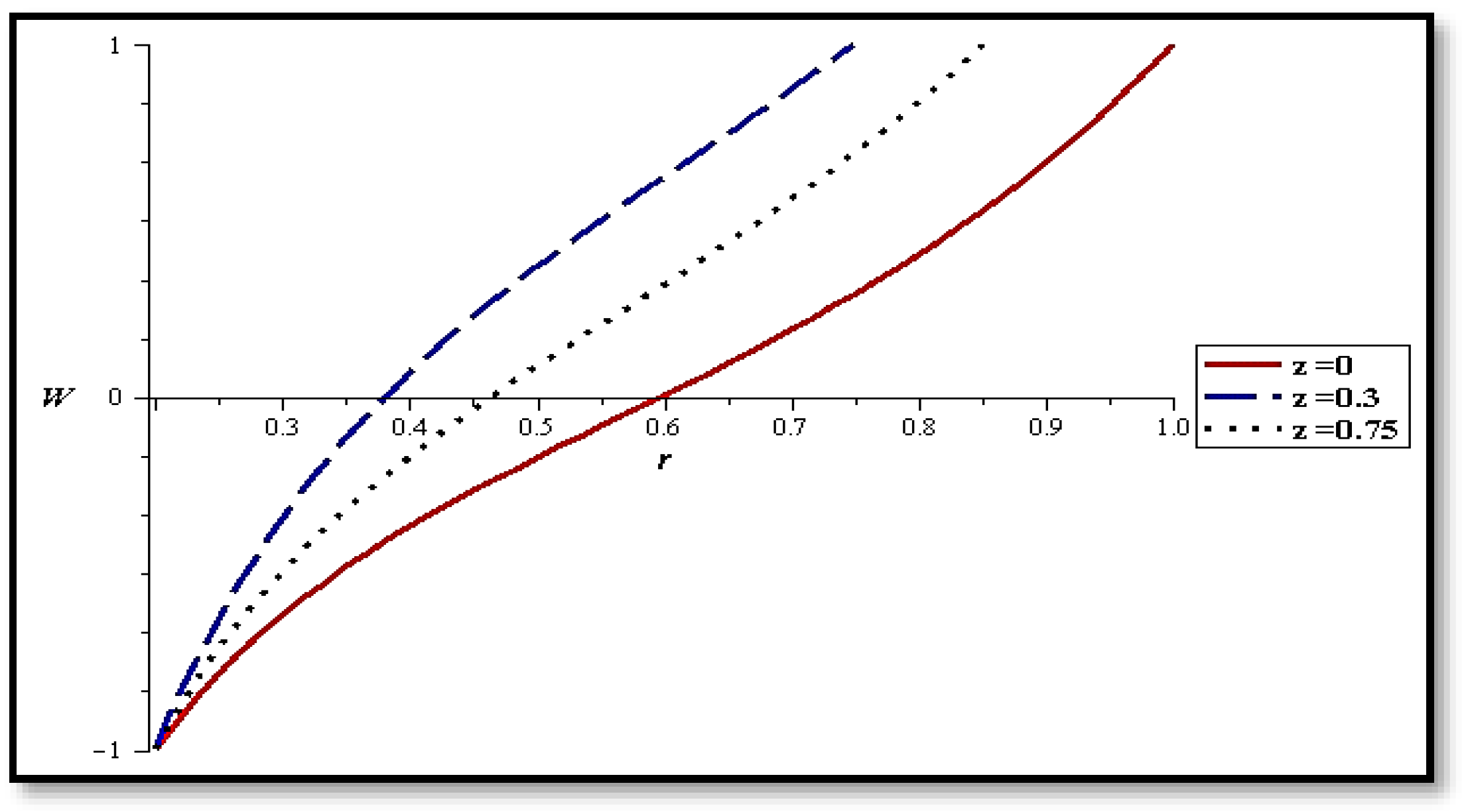
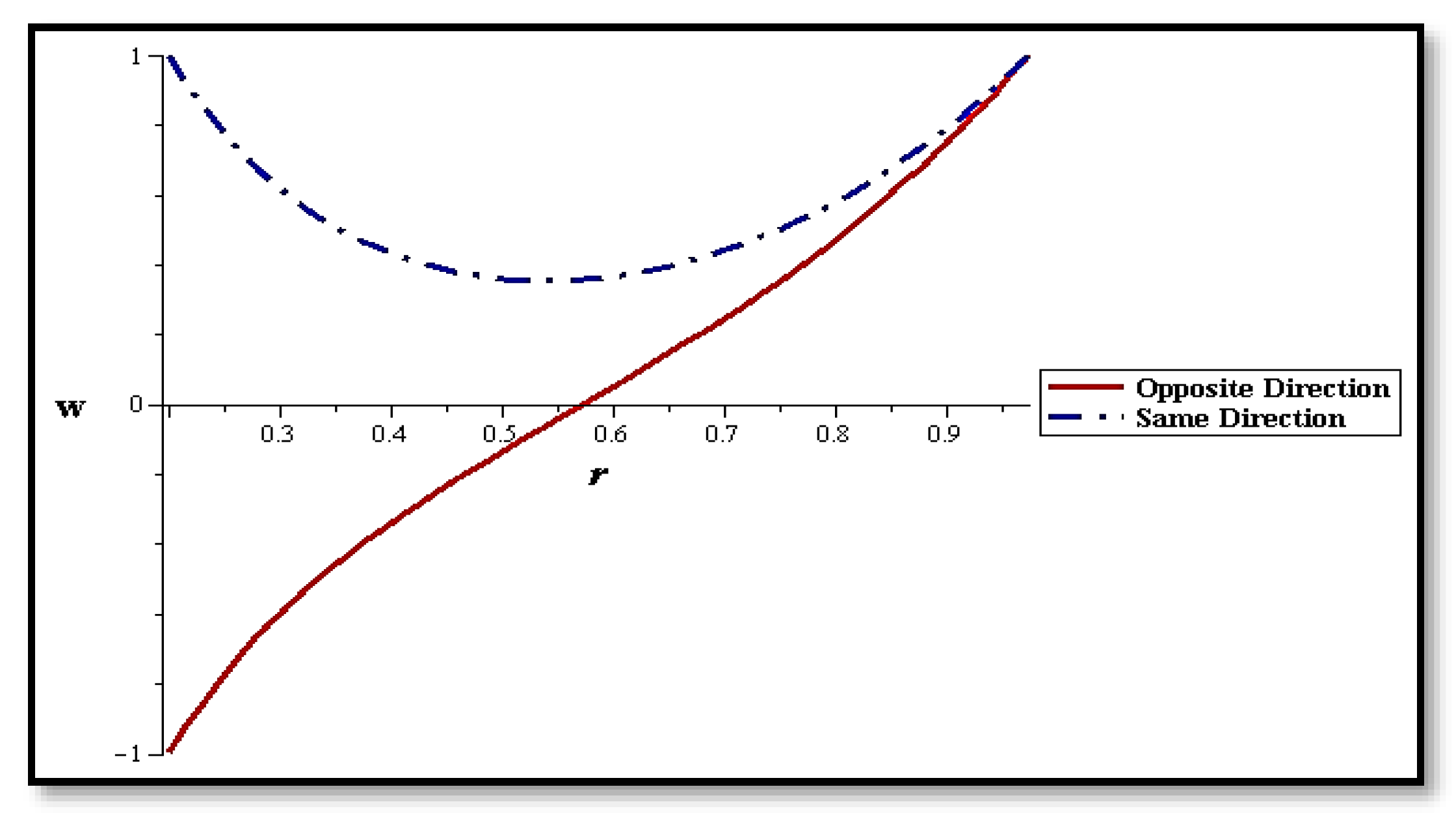
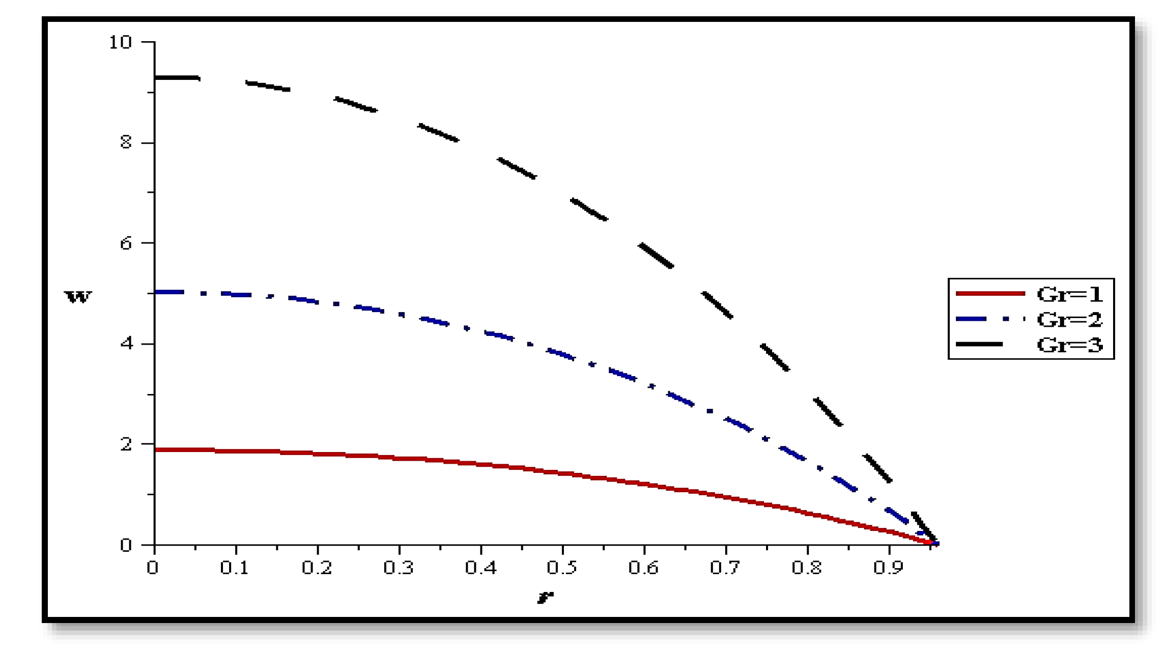
• Velocity increases within the curtailment, whilst during the extension, velocity decreases;
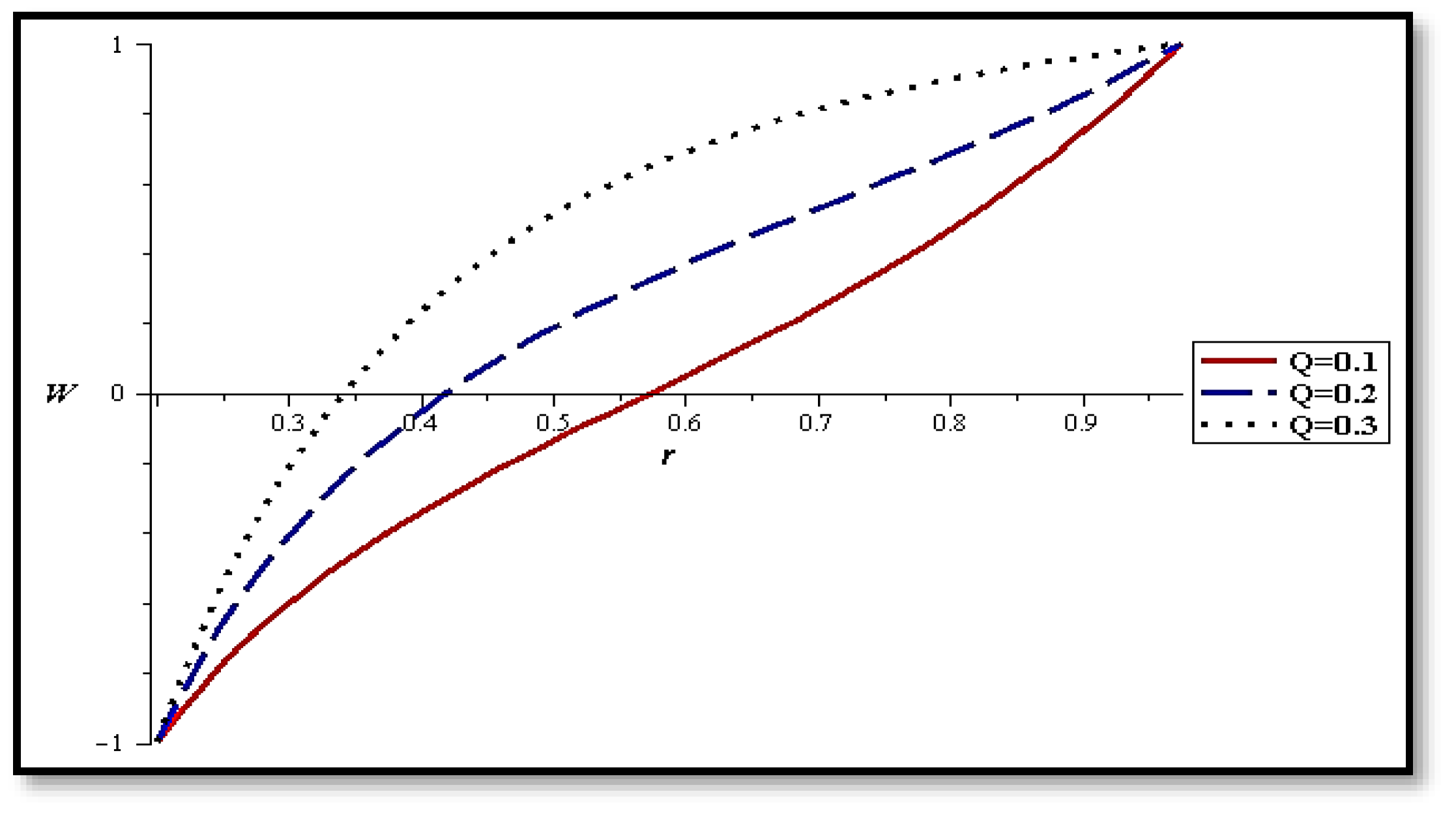
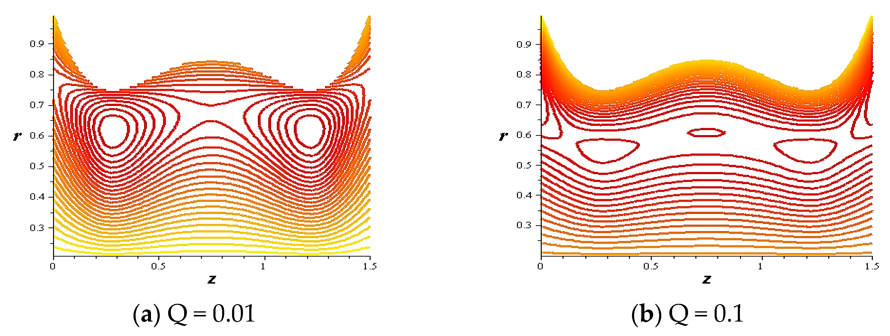
• The flowing rate boosts the velocity behind the artery wall and diminished it at the catheter;
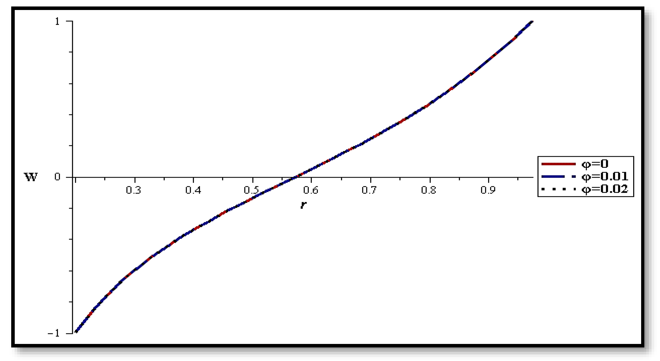
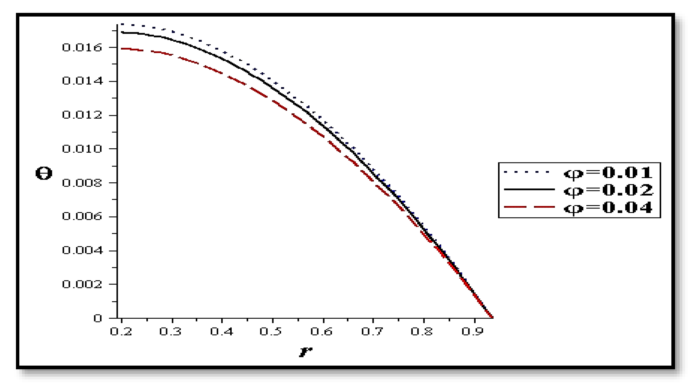
• The nanoparticles concentration has a little effect on the velocity;
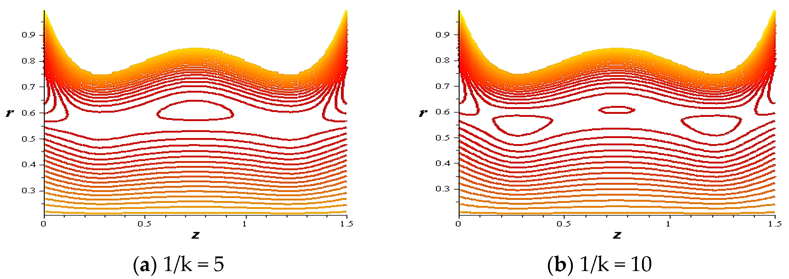
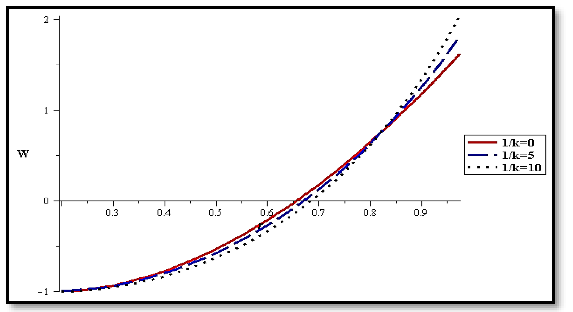
• With porous media the velocity increases at the catheter and decreases at the wall;
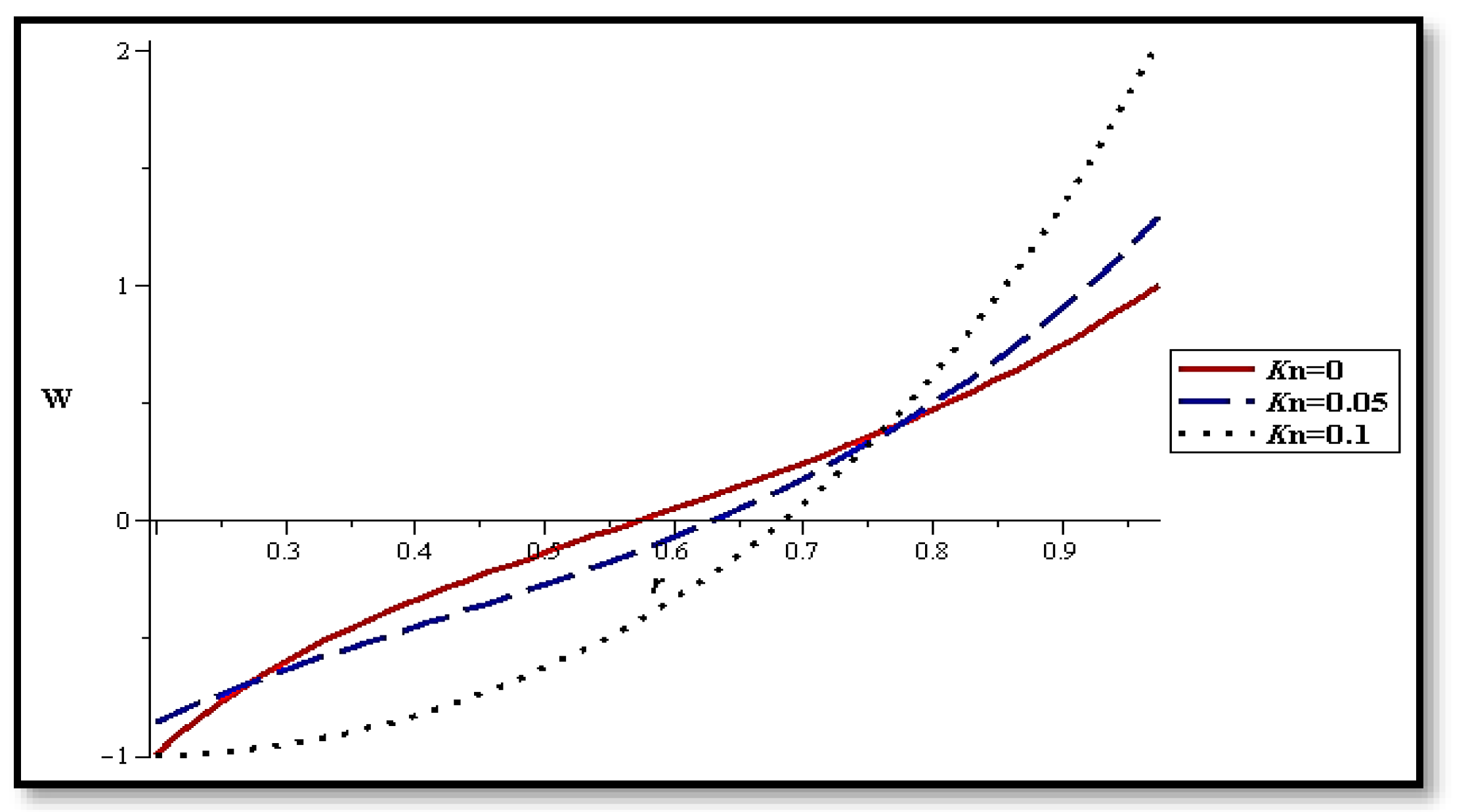
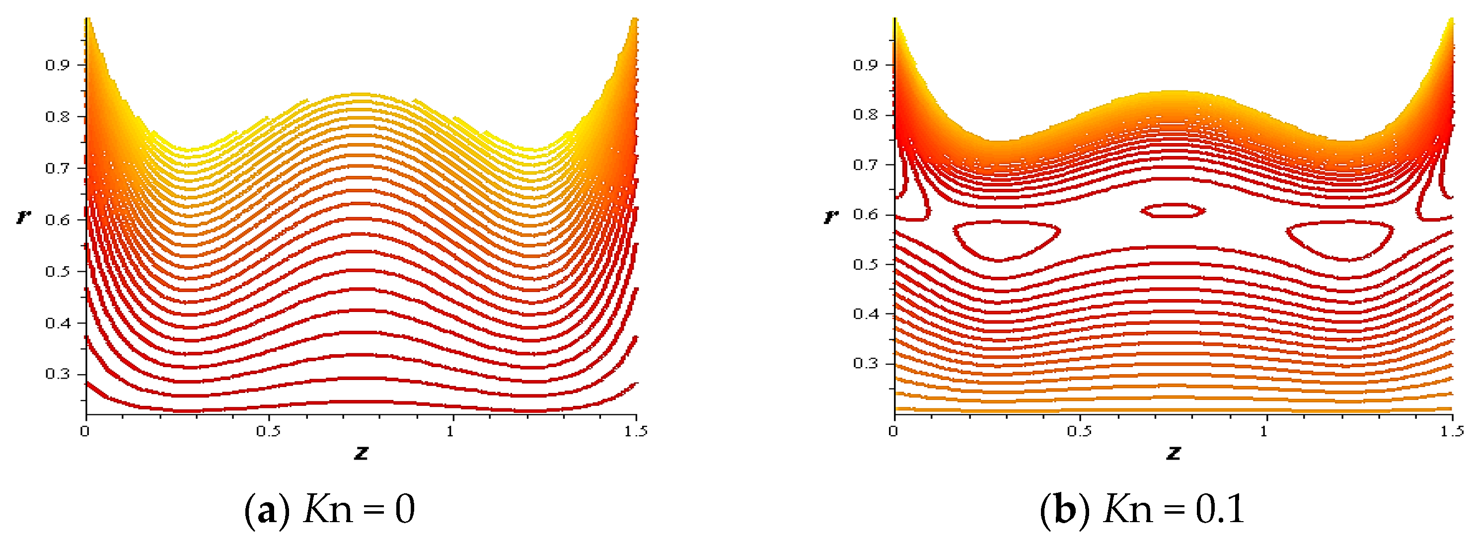
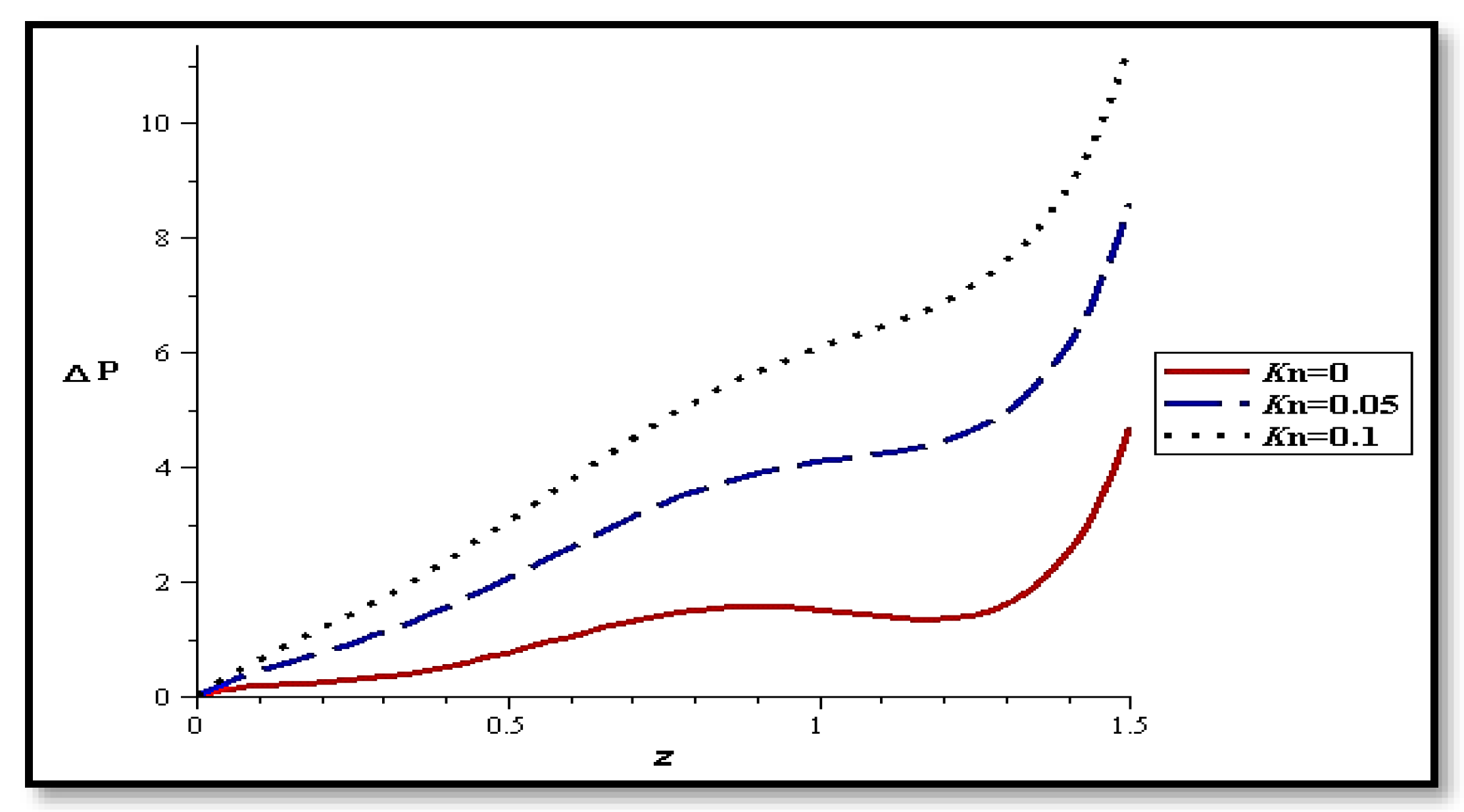
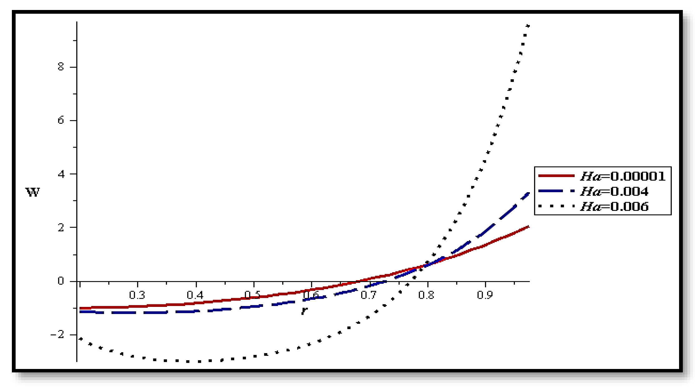
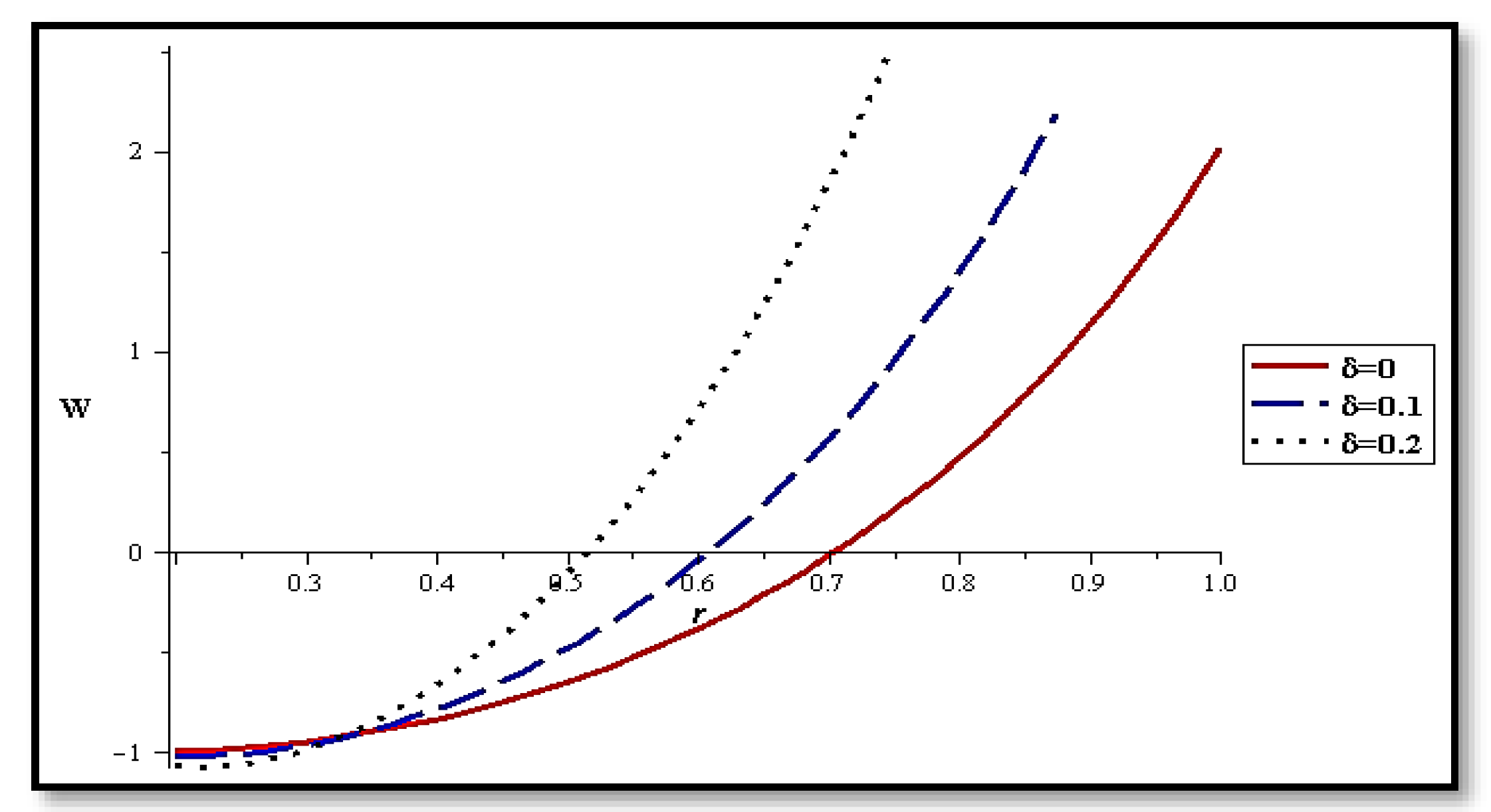
• The velocity increases when increasing the slipping and magnetic field at the wall;
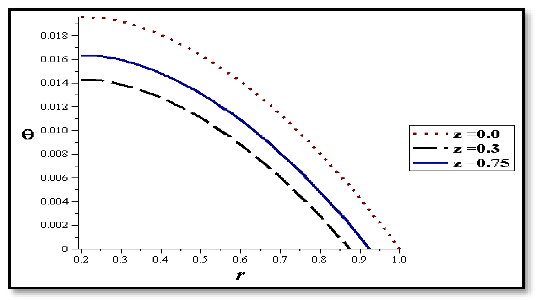
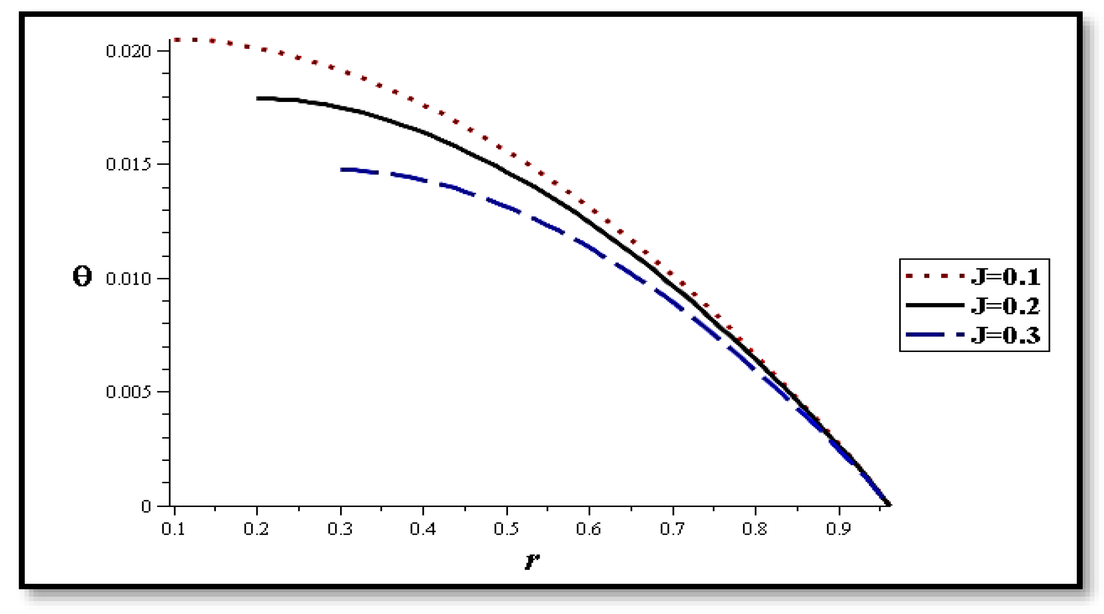
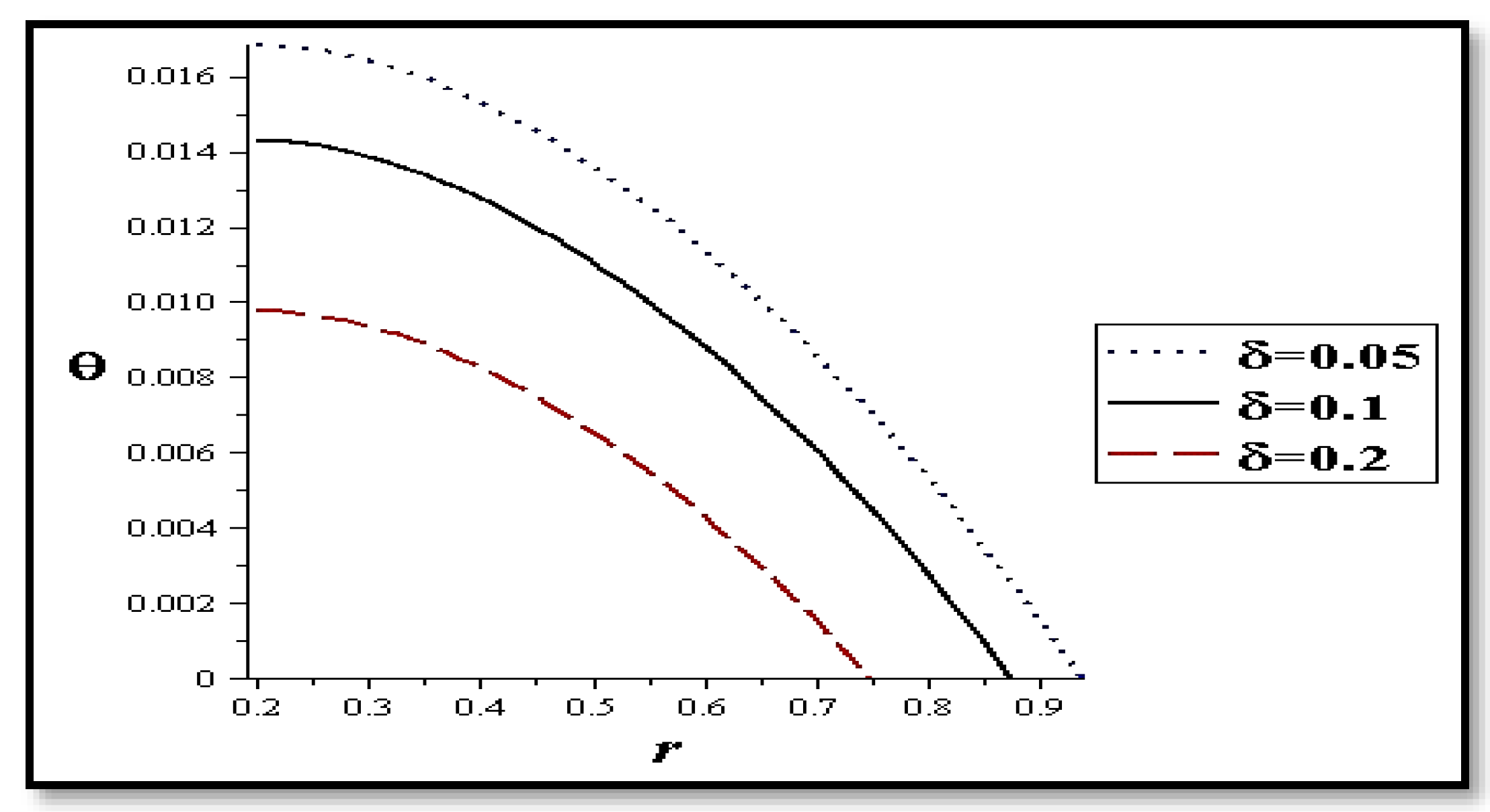
• The temperature decreases within the contraction, whilst increasing within the expansion;
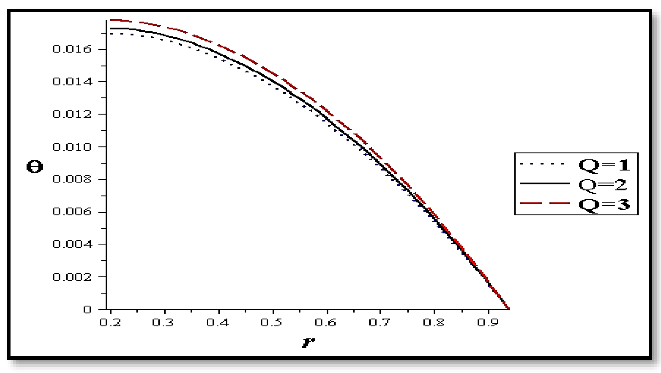
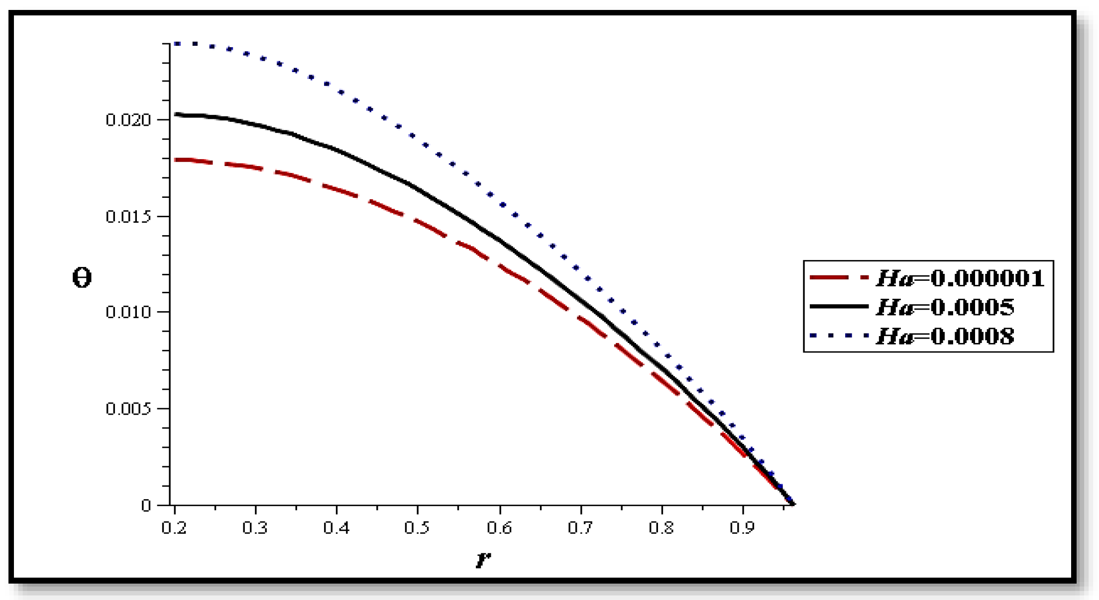
• The inflow rate and magnetic field enhance the thermal energy to the fluid unlike the presence of the catheter;
• The nanoparticles concentration, slipping, and porosity decrease the thermal energy;
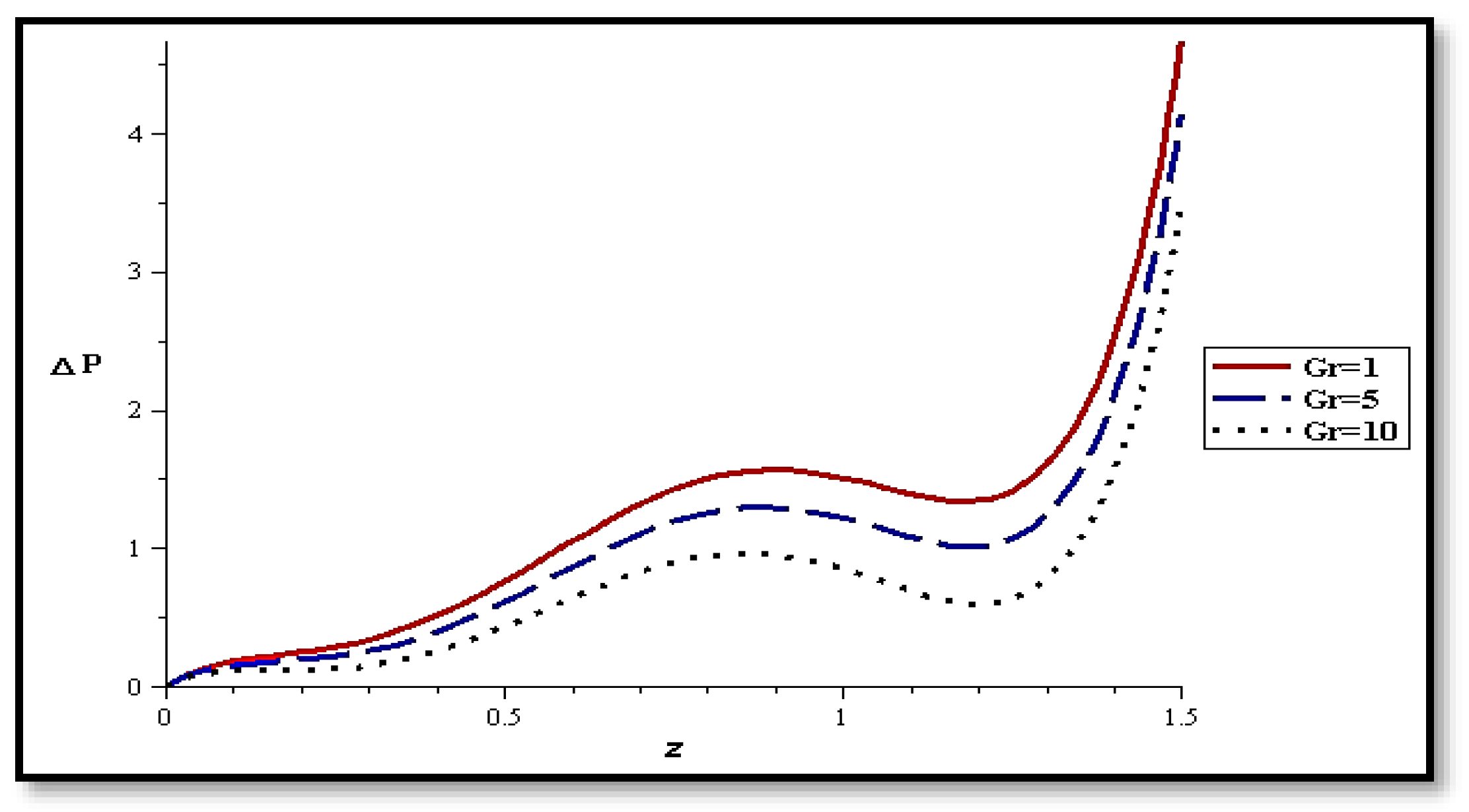
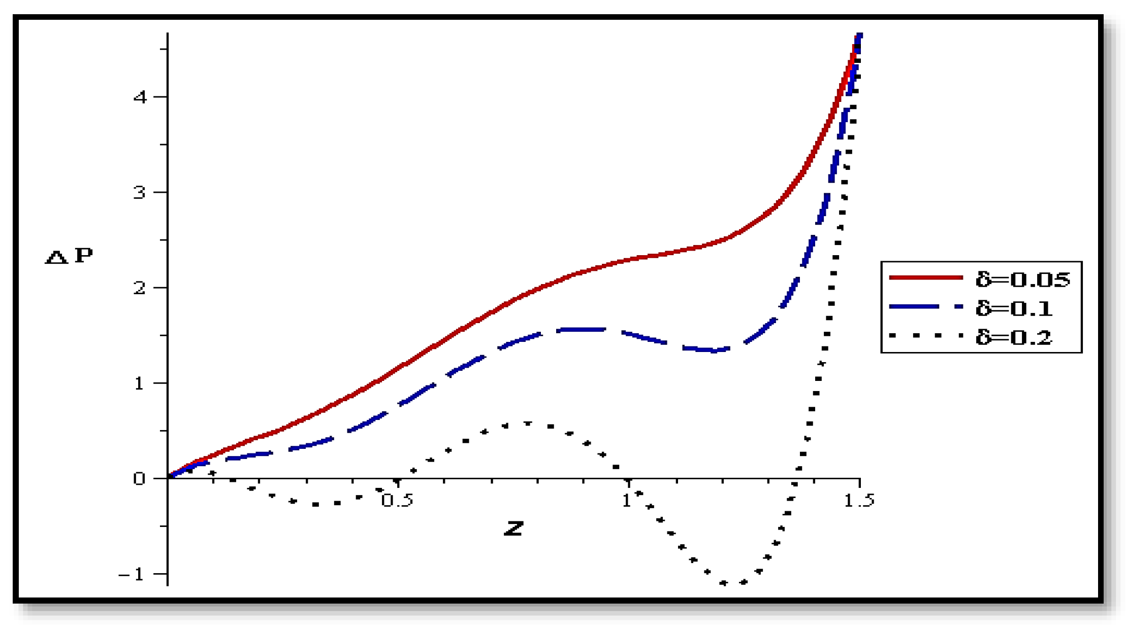
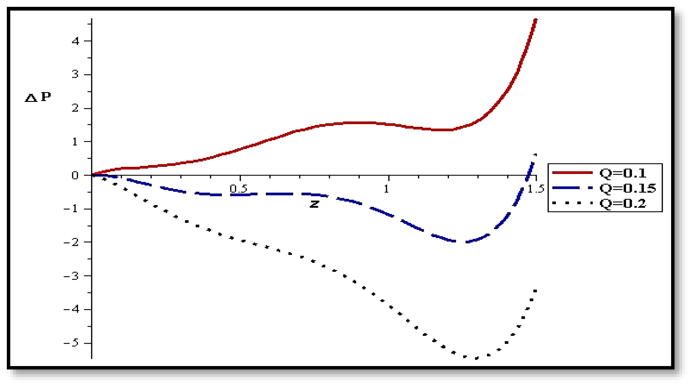
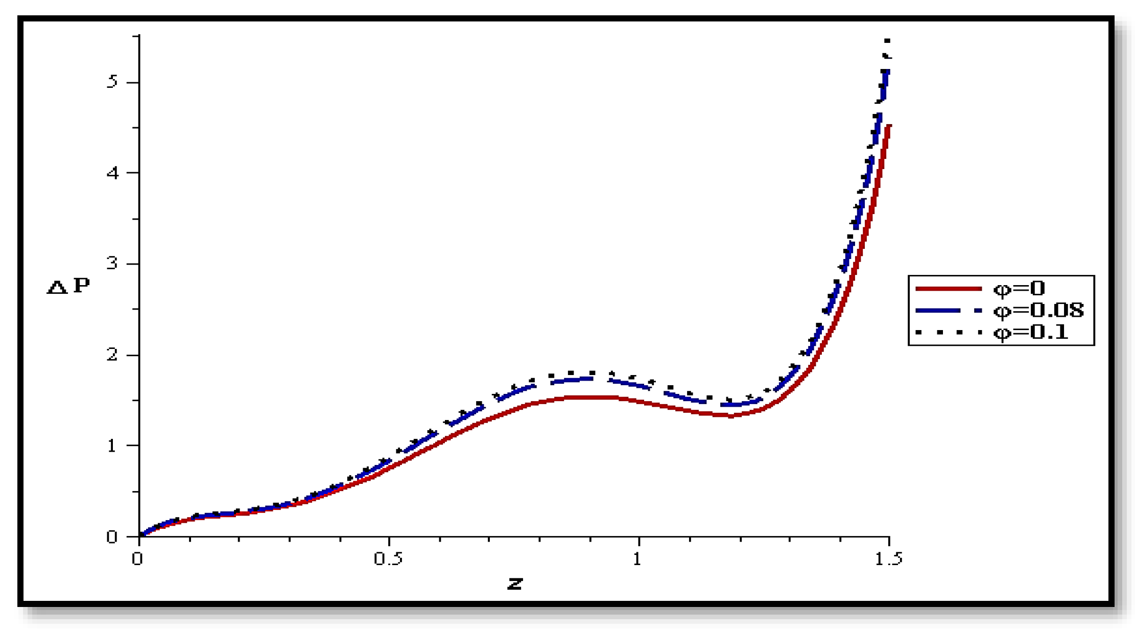
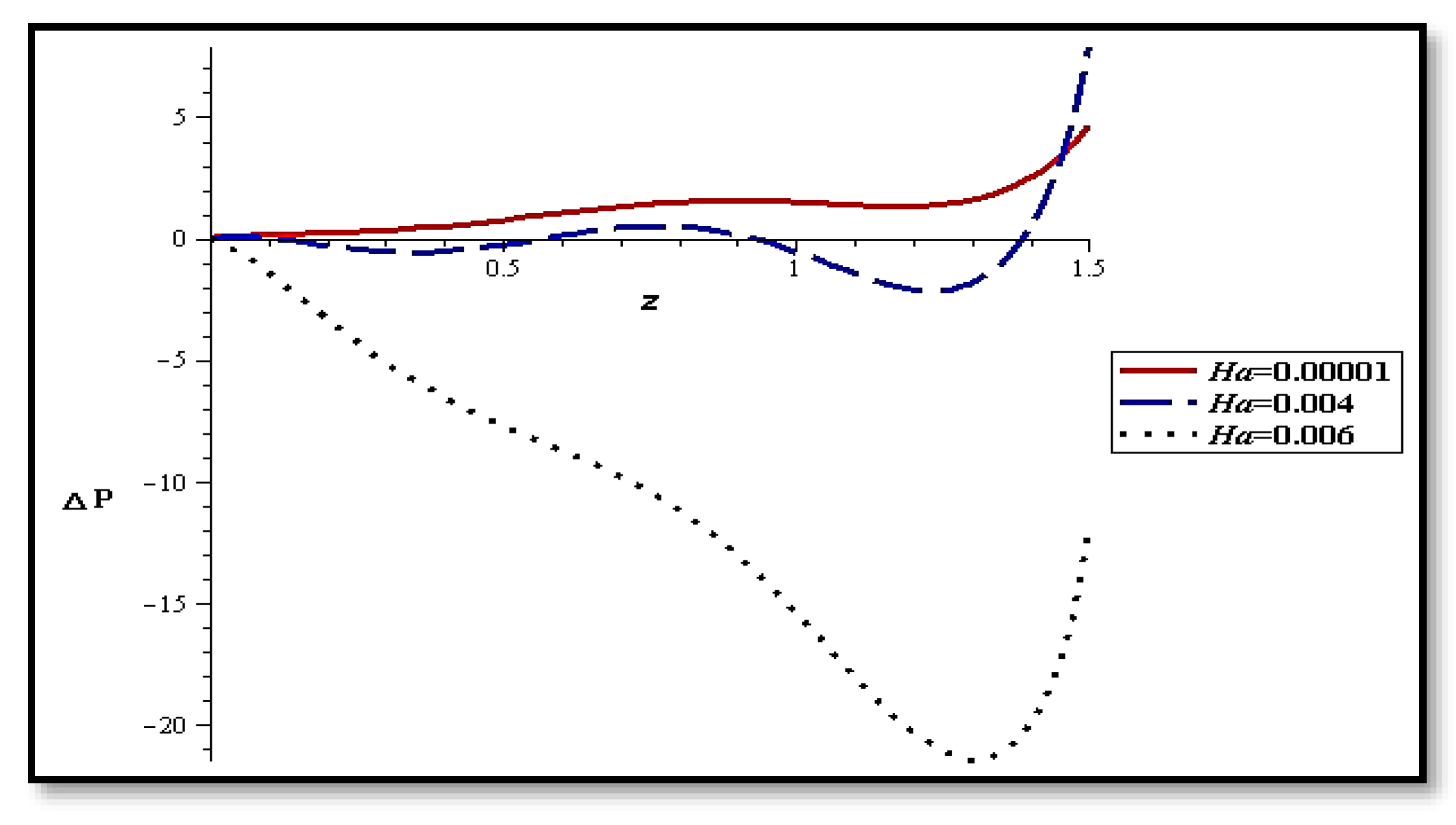
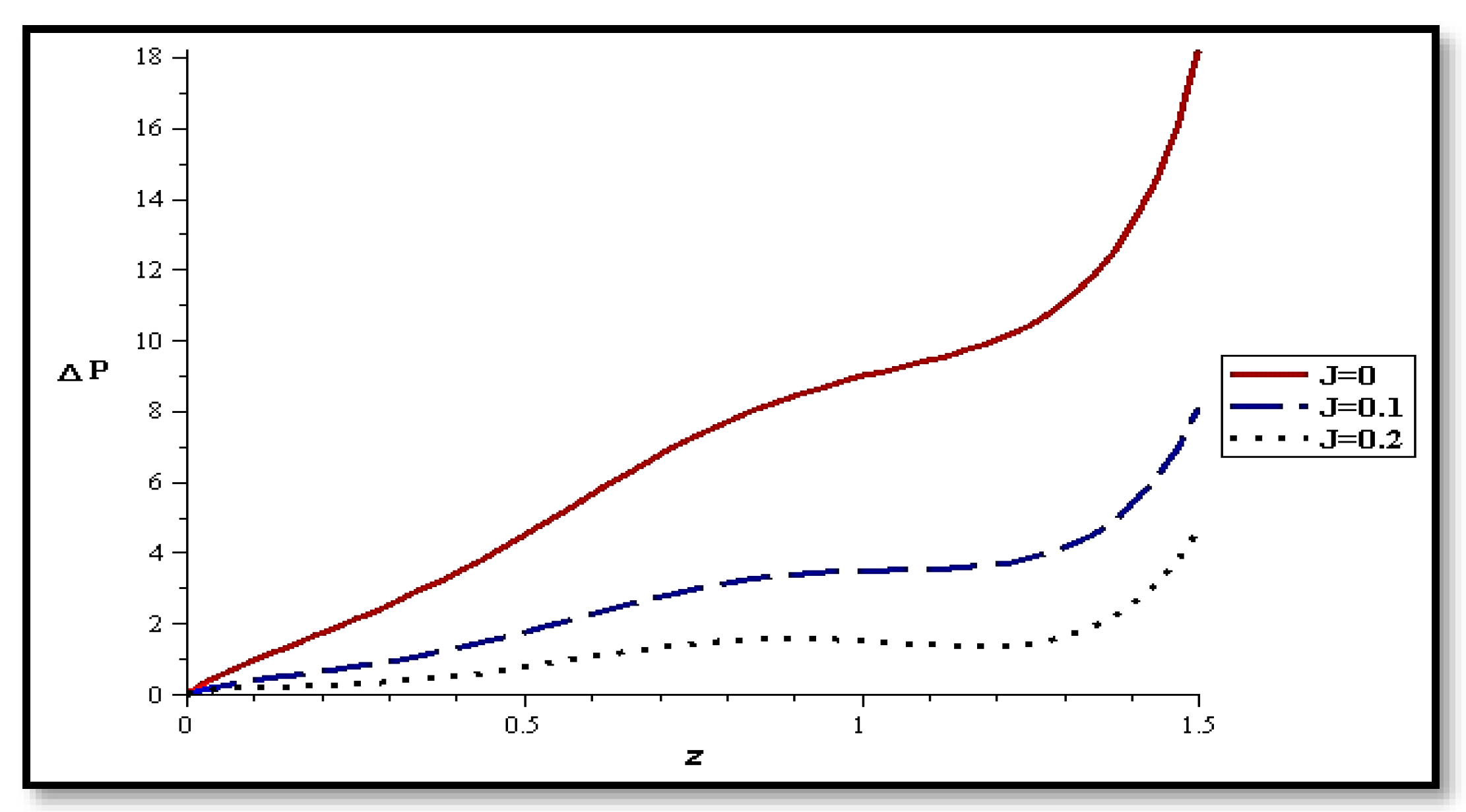
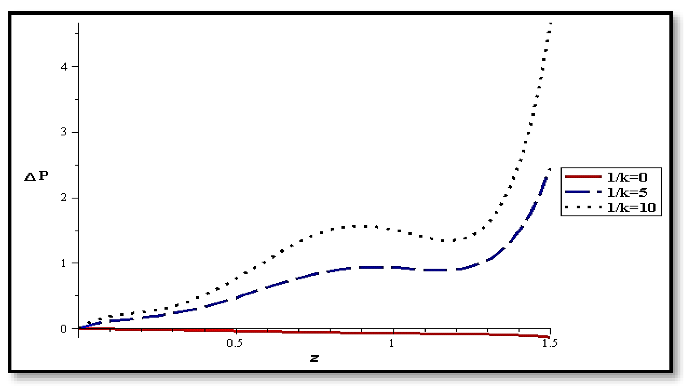
• The presence of amplitude ratio, flow rate, nanoparticles concentration, magnetic field, and slipping increase the pressure difference, unlike the presence of catheter and gravity.

References

1. Pal, S.L.; Jana, U.; Manna, P.K.; Mohanta, G.P.; Manavalan, R. Nanoparticle: An overview of preparation and characterization. J. Appl. Pharm. Sci. 2011, 1, 228–234. [Google Scholar]
2. Akbar, N.S.; Maraj, E.; Butt, A.W. Copper nanoparticles impinging on a curved channel with compliant walls and peristalsis. Eur. Phys. J. Plus 2014, 129, 183. [Google Scholar] [CrossRef]
3. Chu, W.K.-H.; Fang, J. Peristaltic transport in a slip flow. Eur. Phys. J. B Condens. Matter Complex Syst. 2000, 16, 543–547. [Google Scholar] [CrossRef]
4. Eldesoky, I.M. Slip effects on the unsteady MHD pulsatile blood flow through porous medium in an artery under the effect of body acceleration. Int. J. Math. Math. Sci. 2012, 2012, 860239. [Google Scholar] [CrossRef] [Green Version]
5. Eldesoky, I.M.; Kamel, M.H.; Abumandour, R.M. Numerical study of slip effect of unsteady MHD pulsatile flow through porous medium in an artery using generalized differential quadrature method (comparative study). In The International Conference on Mathematics and Engineering Physics; Military Technical College: Cairo, Egypt, 2014. [Google Scholar]
6. Abd Elnaby, M.A.; Haroun, M.H. A new model for study the effect of wall properties on peristaltic transport of a viscous fluid. Commun. Nonlinear Sci. Numer. Simul. 2008, 13, 752–762. [Google Scholar] [CrossRef]
7. Hasany, S.F.; Ahmed, I.; Rajan, J.; Rehman, A. Systematic review of the preparation techniques of iron oxide magnetic nanoparticles. Nanosci. Nanotechnol. 2012, 2, 148–158. [Google Scholar] [CrossRef] [Green Version]
8. Muthu, P.; Kumar, B.R.; Chandra, P. Peristaltic motion of micropolar fluid in circular cylindrical tubes: Effect of wall properties. Appl. Math. Model. 2008, 32, 2019–2033. [Google Scholar] [CrossRef]
9. Sreenadh, S.; Shankar, C.U.; Pallavi, A.R. Effects of wall properties and heat transfer on the peristaltic transport of food bolus through oesophagus—A mathematical model. Int. J. Appl. Math. Mech. 2012, 8, 93–108. [Google Scholar]
10. Hron, J.; Le Roux, C.; Malek, J.; Rajagopal, K. Flows of incompressible fluids subject to Navier’s slip on the boundary. Comput. Math. Appl. 2008, 56, 2128–2143. [Google Scholar] [CrossRef] [Green Version]
11. Abumandour, R.M.; Eldesoky, I.M.; Kamel, M.H.; Ahmed, M.M.; Abdelsalam, S.I. Peristaltic thrusting of a thermal-viscosity nanofluid through a resilient vertical pipe. Z. Nat. A 2020, 75, 727–738. [Google Scholar] [CrossRef]
12. Sharma, M.K.; Bansal, K.; Bansal, S. Pulsatile unsteady flow of blood through porous medium in a stenotic artery under the influence of transverse magnetic field. Korea-Aust. Rheol. J. 2012, 24, 181–189. [Google Scholar] [CrossRef]
13. Sucharitha, G.; Lakshminarayana, P.; Sandeep, N. MHD and Cross Diffusion Effects on Peristaltic Flow of a Casson Nanofluid in a Duct. Appl. Math. Sci. Comput. 2019, 2, 191–201. [Google Scholar]
14. Akbar, N.S. Metallic Nanoparticles Analysis for the Peristaltic Flow in an Asymmetric Channel with MHD. IEEE Trans. Nanotechnol. 2014, 13, 357–361. [Google Scholar] [CrossRef]
15. Sucharitha, G.; Vajravelu, K.; Lakshminarayana, P. Effect of heat and mass transfer on the peristaltic flow of a Jeffrey nanofluid in a tapered exible channel in the presence of aligned magnetic field. Eur. Phys. J. Spec. Top. 2019, 228, 2713–2728. [Google Scholar] [CrossRef]
16. Bejan, A. Entropy generation minimization: The new thermodynamics of finite-size devices and finite-time processes. J. Appl. Phys. 1996, 79, 1191–1218. [Google Scholar] [CrossRef] [Green Version]
17. Khan, W.A.; Ali, M. Recent developments in modeling and simulation of entropy generation for dissipative cross material with quartic autocatalysis. Appl. Phys. A 2019, 125, 397. [Google Scholar] [CrossRef]
18. Rashidi, M.M.; Bhatti, M.M.; Abbas, M.A.; Ali, M.E.-S. Entropy generation on MHD blood flow of nanofluid due to peristaltic waves. Entropy 2016, 18, 117. [Google Scholar] [CrossRef] [Green Version]
19. Hayat, T.; Rafiq, M.; Ahmad, B.; Asghar, S. Entropy generation analysis for peristaltic flow of nanoparticles in a rotating frame. Int. J. Heat Mass Transf. 2017, 108, 1775–1786. [Google Scholar] [CrossRef]
20. Ranjit, N.K.; Shit, G.C. Entropy generation on electroosmotic flow pumping by a uniform peristaltic wave under magnetic environment. Energy 2017, 128, 649–660. [Google Scholar] [CrossRef]
21. Ali, M.; Khan, W.A.; Irfan, M.; Sultan, F.; Shahzed, M.; Khan, M. Computational analysis of entropy generation for cross-nanofluid flow. Appl. Nanosci. 2019, 10, 3045–3055. [Google Scholar] [CrossRef]
22. Borges, M.E.; Sierra, M.; Cuevas, E.; García, R.; Esparza, P. Photocatalysis with solar energy: Sunlight-responsive photocatalyst based on TiO2 loaded on a natural material for wastewater treatment. Sol. Energy 2016, 135, 527–535. [Google Scholar] [CrossRef]
23. Zhang, H.; Yang, H.; Chen, H.; Du, X.; Wen, D.; Wu, H. Photothermal conversion characteristics of gold nanoparticles under different filter conditions. Sol. Energy 2014, 100, 141–147. [Google Scholar] [CrossRef]
24. Zeiny, A.; Jin, H.; Bai, L.; Lin, G.; Wen, D. A comparative study of direct absorption nanfoluids for solar thermal applications. Sol. Energy 2018, 161, 74–82. [Google Scholar] [CrossRef]
25. Shi, L.; He, Y.; Wang, X.; Hu, Y. Recyclable photo-thermal conversion and purification systems via Fe3O4@TiO2 nanoparticles. Energy Convers. Manag. 2018, 171, 272–278. [Google Scholar] [CrossRef]
26. Prakash, J.; Siva, E.; Tripathi, D.; Kuharat, S.; Bég, O.A. Peristaltic pumping of magnetic nanofluids with thermal radiation and temperature-dependent viscosity effects: Modelling a solar magneto-biomimetic nanopump. Renew. Energy 2018, 133, 1308–1326. [Google Scholar] [CrossRef]
27. Prakash, J.; Ramesh, K.; Tripathi, D.; Kumar, R. Numerical simulation of heat transfer in blood flow altered by electroosmosis through tapered micro-vessels. Microvasc. Res. 2018, 118, 162–172. [Google Scholar] [CrossRef] [PubMed]
28. Hina, S.; Mustafa, M.; Hayat, T.; Alsaedi, A. Peristaltic transport of Powell–Eyring fluid in a curved channel with heat/mass transfer and wall properties. Int. J. Heat Mass Transf. 2016, 101, 156–165. [Google Scholar] [CrossRef]
29. Kumar, M.A.; Sreenadh, S.; Srinivas, A.N.S. Effects of wall properties and heat transfer on the peristaltic transport of a jeffrey fluid in a channel. Adv. Appl. Sci. Res. 2013, 6, 156–172. [Google Scholar]
30. Reddy, M.G. Heat and mass transfer on magnetohydrodynamic peristaltic flow in a porous medium with partial slip. Alex. Eng. J. 2016, 55, 1225–1234. [Google Scholar] [CrossRef]
31. Suganya, S.; Muthtamilselvan, M.; Al-Amri, F.; Abdalla, B. An exact solution for unsteady free convection flow of chemically reacting Al2O3-SiO2/Water hybrid nanofluid. J. Mech. Eng. Sci. 2020, 235, 3749–3763. [Google Scholar] [CrossRef]
32. Hayat, T.; Shafique, M.; Tanveer, A.; Alsaedi, A. Magnetohydrodynamic effects on peristaltic flow of hyperbolic tangent nanofluid with slip conditions and Joule heating in an inclined channel. Int. J. Heat Mass Transf. 2016, 102, 54–63. [Google Scholar] [CrossRef]
33. Ramesh, K.; Devakar, M. Magnetohydrodynamic peristaltic transport of couple stress fluid through porous medium in an inclined asymmetric channel with heat transfer. J. Magn. Magn. Mater. 2015, 394, 335–348. [Google Scholar] [CrossRef]
34. Hayat, T.; Farooq, S.; Alsaedi, A.; Ahmad, B. Hall and radial magnetic field effects on radiative peristaltic flow of Carreau–Yasuda fluid in a channel with convective heat and mass transfer. J. Magn. Magn. Mater. 2016, 412, 207–216. [Google Scholar] [CrossRef]
35. Misra, J.; Mallick, B.; Sinha, A. Heat and mass transfer in asymmetric channels during peristaltic transport of an MHD fluid having temperature-dependent properties. Alex. Eng. J. 2018, 57, 391–406. [Google Scholar] [CrossRef] [Green Version]
36. Hayat, T.; Riaz, A.; Tanveer, A.; Alsaedi, A. Peristaltic transport of tangent hyperbolic fluid with variable viscosity. Therm. Sci. Eng. Prog. 2018, 6, 217–225. [Google Scholar] [CrossRef]
37. Shaheen, A.; Asjad, M.I. Peristaltic flow of a Sisko fluid over a convectively heated surface with viscous dissipation. J. Phys. Chem. Solids 2018, 122, 210–217. [Google Scholar] [CrossRef]
38. Kothandapani, M.; Srinivas, S. On the influence of wall properties in the MHD peristaltic transport with heat transfer and porous medium. Phys. Lett. A 2008, 372, 4586–4591. [Google Scholar] [CrossRef]
39. Shapiro, A.H.; Jaffrin, M.Y.; Weinberg, S.L. Peristaltic pumping with long wavelengths at low Reynolds number. J. Fluid Mech. 1969, 37, 799–825. [Google Scholar] [CrossRef]
40. Mekheimer, K.S.; Mohamed, M.S.; Elnaqeeb, T. Metallic nanoparticles influence on blood flow through a stenotic artery. Int. J. Pure Appl. Math. 2016, 107, 201. [Google Scholar] [CrossRef]
Figure 1. Problem modeling.
Mathematics 10 00492 g001
Figure 2. Velocity with different gravity at (Kn = 0, S = 0.1, k = 0.1, Ha = 1.5, J = 0, Q = 0.1, δ = 0.05, φ = 0.02).
Mathematics 10 00492 g002
Figure 3. Velocity at different locations at (Kn = 0, Gr = 1, φ = 0.02, S = 0.1, k = 0.1, Ha = 10−5, J = 0.2, Q = 0.1, δ = 0.02).
Mathematics 10 00492 g003
Figure 4. Velocity with different flow rates at (Kn = 0, φ = 0.02, S = 0.1, k = 0.1, Ha = 10−5, J = 0.2, δ = 0.02).
Mathematics 10 00492 g004
Figure 5. Velocity with different nanoparticles concentrations at (Kn = 0, S = 0.1, k = 0.1, Ha = 10−5, J = 0.2, Q = 0.2, δ = 0.02).
Mathematics 10 00492 g005
Figure 6. Velocity variations with Kn at (φ = 0.02, S = 0.1, k = 0.1, Ha = 10−5, J = 0.2, Q = 0.1, δ = 0.02).
Mathematics 10 00492 g006
Figure 7. Velocity with Ha at (Kn = 0.1, φ = 0.01, S = 0.1, k = 0.1, J = 0.2, Q = 0.1, δ = 0.02).
Mathematics 10 00492 g007
Figure 8. Velocity with porosity at (Kn = 0.1, φ = 0.01, S = 0.1, k = 0.1, Ha = 10−5, J = 0.2, Q = 0.1, δ = 0.02).
Mathematics 10 00492 g008
Figure 9. Velocity with catheter sizes at (Kn = 0.1, φ = 0.01, S = 0.1, k = 0.1, Ha = 10−5, δ = 0.02, Q = 0.1, Gr = 1).
Mathematics 10 00492 g009
Figure 10. Velocity with different amplitude ratios at (Kn = 0.1, Ha = 10−5, J = 0.2, φ = 0.01, S = 0.1, k = 0.1, Q = 0.1, Gr = 1).
Mathematics 10 00492 g010
Figure 11. Velocity distribution with reverse catheter movement at (Kn = 0, Ha = 10−5, J = 0.2, φ = 0.02, S = 0.1, k = 0.1, Q = 0.1, Gr = 1).
Mathematics 10 00492 g011
Figure 12. Streamlines with flow rate at (Kn = 0.1, J = 0.2, φ = 0.02, k = 0.1, δ = 0.2, S = 0.1, Q = 0.1, Ha = 10−5, Gr = 1).
Mathematics 10 00492 g012
Figure 13. Streamlines with the Knudsen number at (J = 0.2, φ = 0.02, k = 0.1, δ = 0.2, S = 0.1, Q = 0.1, Ha = 10−5, Gr = 1).
Mathematics 10 00492 g013
Figure 14. Streamlines with porosity at (Kn = 0.1, J = 0.2, φ = 0.02, δ = 0.2, S = 0.1, Q = 0.1, Ha = 10−5, Gr = 1).
Mathematics 10 00492 g014
Figure 15. Streamlines with magnetic field at (Kn = 0.1, J = 0.2, φ = 0.02, k = 0.1, δ = 0.2, S = 0.1, Q = 0.1, Gr = 1).
Mathematics 10 00492 g015
Figure 16. Temperature profiles with different locations at (Kn = 0.1, J = 0.2, φ = 0.02, δ = 0.1, S = 0.1, Q = 0.1, Ha = 10−5, Gr = 1, Br = 0.1, k = 0.1).
Mathematics 10 00492 g016
Figure 17. Temperature profiles with the flow rate at (Kn = 0.1, J = 0.2, φ = 0.02, δ = 0.1, S = 0.1, Ha = 10−5, Gr = 1, Br = 0.1, k = 0.1).
Mathematics 10 00492 g017
Figure 18. Temperature profiles with nanoparticles concentration at (Kn = 0.1, J = 0.2, δ = 0.05, S = 0.1, Ha = 10−5, Gr = 0.1, Br = 0.1, k = 0.1, Q = 0.1).
Mathematics 10 00492 g018
Figure 19. Temperature profiles with the Hartman number at (φ = 0.02, Kn = 0.1, J = 0.2, δ = 0.05, S = 0.1, Gr = 0.1, Br = 0.1, k = 0.1, Q = 0.1).
Mathematics 10 00492 g019
Figure 20. Temperature profiles with the catheter size at (φ = 0.02, Kn = 0.1, δ = 0.05, S = 0.1, Gr = 0.1, Br = 0.1, k = 0.1, Q = 0.1, Ha = 10−5).
Mathematics 10 00492 g020
Figure 21. Temperature profiles with the amplitude ratio at (φ = 0.02, J = 0.2, Ha = 10−5, Kn = 0.1, S = 0.1, Gr = 0.1, Br = 0.1, k = 0.1, Q = 0.1).
Mathematics 10 00492 g021
Figure 22. Pressure difference profiles vs. positions at different amplitude ratios (φ = 0.02, J = 0.2, S = 0.1, Ha = 10−5, Kn = 0, Gr = 1, k = 0.1, Q = 0.1).
Mathematics 10 00492 g022
Figure 23. Pressure difference profiles vs. positions at different flow rates (φ = 0.02, δ = 0.1, Ha = 10−5, J = 0.2, Kn = 0, S = 0.1, Gr = 1, k = 0.1, Q = 0.1).
Mathematics 10 00492 g023
Figure 24. Pressure difference profiles vs. positions at different nanoparticle concentrations (δ = 0.1, k = 0.1, Ha = 10−5, J = 0.2, Kn = 0, S = 0.1, Gr = 1, Q = 0.1).
Mathematics 10 00492 g024
Figure 25. Pressure difference profiles vs. positions at different slip parameters (φ = 0.02, δ = 0.1, J = 0.2, Ha = 10−5, S = 0.1, Gr = 1, k = 0.1, Q = 0.1).
Mathematics 10 00492 g025
Figure 26. Pressure difference profiles vs. positions at different magnetic fields (Kn = 0, φ = 0.02, δ = 0.1, J = 0.2, S = 0.1, Gr = 1, k = 0.1, Q = 0.1).
Mathematics 10 00492 g026
Figure 27. Pressure difference profiles vs. positions at different catheter sizes (Kn = 0, φ = 0.02, δ = 0.1, Ha = 10−5, S = 0.1, Gr = 1, k = 0.1, Q = 0.1).
Mathematics 10 00492 g027
Figure 28. Pressure difference profiles vs. positions at different porosities (Kn = 0, φ = 0.02, δ = 0.1, Ha = 10−5, S = 0.1, Gr = 1, J = 0.2, Q = 0.1).
Mathematics 10 00492 g028
Figure 29. Pressure difference profiles vs. positions at different gravity (Kn = 0, φ = 0.02, δ = 0.1, J = 0.2, Ha = 10−5, S = 0.1, k = 0.1, Q = 0.1).
Mathematics 10 00492 g029