A Generic Model in Which the Russell-Nontypical Sets Satisfy ZFC Strictly between HOD and the Universe

Abstract

The notion of ordinal definability and the related notions of ordinal definable sets (class $\mathbf{OD}$) and hereditarily ordinal definable sets (class $\mathbf{HOD}$) belong to the key concepts of modern set theory. Recent studies have discovered more general types of sets, still based on the notion of ordinal definability, but in a more blurry way. In particular, Tzouvaras has recently introduced the notion of sets nontypical in the Russell sense, so that a set x is nontypical if it belongs to a countable ordinal definable set. Tzouvaras demonstrated that the class $\mathbf{HNT}$ of all hereditarily nontypical sets satisfies all axioms of $\mathbf{ZF}$ and satisfies $\mathbf{HOD}\subseteq \mathbf{HNT}$. In view of this, Tzouvaras proposed a problem—to find out whether the class $\mathbf{HNT}$ can be separated from $\mathbf{HOD}$ by the strict inclusion $\mathbf{HOD}⫋\mathbf{HNT}$, and whether it can also be separated from the universe $\mathbf{V}$ of all sets by the strict inclusion $\mathbf{HNT}⫋\mathbf{V}$, in suitable set theoretic models. Solving this problem, a generic extension $\mathbf{L}[a,x]$ of the Gödel-constructible universe $\mathbf{L}$, by two reals $a,x$, is presented in this paper, in which the relation $\mathbf{L}=\mathbf{HOD}⫋\mathbf{L}\left[a\right]=\mathbf{HNT}⫋\mathbf{L}[a,x]=\mathbf{V}$ is fulfilled, so that $\mathbf{HNT}$ is a model of $\mathbf{ZFC}$ strictly between $\mathbf{HOD}$ and the universe. Our result proves that the class $\mathbf{HNT}$ is really a new rich class of sets, which does not necessarily coincide with either the well-known class $\mathbf{HOD}$ or the whole universe $\mathbf{V}$. This opens new possibilities in the ongoing study of the consistency and independence problems in modern set theory.

1. Introduction

We recall that a set X is ordinal definable if X can be defined by a formula with ordinals as parameters in the universe of all sets. The class of all ordinal definable sets is denoted by $\mathbf{OD}$. Further, a set X is hereditarily ordinal definable if X itself, as well as all elements of X, all elements of elements of X, etc., belong to $\mathbf{OD}$. In other words, it is required that $\mathrm{TC}\left(X\right)\subseteq \mathbf{OD}$, where $\mathrm{TC}\left(X\right)$, the transitive closure of X, is the least transitive set containing X, and a set Y is transitive if $x\in y\in Y⟹x\in Y$. The class of all hereditarily ordinal definable sets is denoted by $\mathbf{HOD}$. To conclude,

$$\begin{array}{ccc}\hfill \mathbf{OD}& =& \left\{x:x\mathrm{is}\mathrm{ordinal}\mathrm{definable}\right\}\hfill \\ \hfill \mathbf{HOD}& =& \left\{x:\mathrm{TC}\right(x)\subseteq \mathbf{OD}\}\hfill \end{array}$$

See more on these fundamental notions of modern set theory in [1] (Chapter 13) or [2] (Section II.8), or [3] as the original reference. In particular, it is known that $\mathbf{HOD}$ is a transitive class and a model of the set theory $\mathbf{ZFC}$ (with the axiom of choice $\mathbf{AC}$). In general, classes $\mathbf{OD}$ and $\mathbf{HOD}$, as well as Gödel’s class $\mathbf{L}$ of all constructible sets, have played a key role in modern set theory since its early days.

Research in recent years has brought to the fore some other notions of definability, such as algebraic definability studied in [4,5,6], blurry definability of [7], and finally nontypicality in the sense of Russell, introduced by Tzouvaras [8,9]. Our paper is dedicated to this last concept. By Tzouvaras, a set x is nontypical, for short $x\in \mathbf{NT}$, if it belongs to a countable ordinal definable set Y. A set x is hereditarily nontypical, for short $x\in \mathbf{HNT}$, if it itself, all its elements, elements of elements, and so on, are all nontypical—in other words, it is required that the transitive closure $\mathrm{TC}\left(x\right)$ satisfy $\mathrm{TC}\left(x\right)\subseteq \mathbf{NT}$. To conclude,

$$\begin{array}{ccc}\hfill \mathbf{NT}& =& \left\{x:\exists Y\right(Y\mathrm{is}\mathrm{countable}\mathrm{and}\mathrm{ordinal}\mathrm{definable},\mathrm{and}x\in Y\left)\right\}\hfill \\ \hfill \mathbf{HNT}& =& \left\{x:\mathrm{TC}\right(x)\subseteq \mathbf{NT}\}\hfill \end{array}$$

Tzouvaras [8,9] connected these notions with some philosophical and mathematical ideas of Bertrand Russell and works of van Lambalgen [10] et al. on the concept of randomness. They contribute to the ongoing study of important classes of sets in the set theoretic universe $\mathbf{V}$ which themselves satisfy the axioms of set theory, similarly to Gödel’s class $\mathbf{L}$ and the class $\mathbf{HOD}$. The class $\mathbf{HNT}$ is transitive and, as shown in [9], satisfies all axioms of $\mathbf{ZF}$ (the axiom of choice AC not included).

It is customary in modern set theory (see e.g., [1,2,11,12]) that any new class of sets is checked in terms of relations with already known classes. In that respect, Tzouvaras [9] established the non-strict inclusion $\mathbf{HOD}\subseteq \mathbf{HNT}$, and proposed a problem: to find out whether the class $\mathbf{HNT}$ can be separated from $\mathbf{HOD}$ by the strict inclusion $\mathbf{HOD}⫋\mathbf{HNT}$, and can also be separated from the universe $\mathbf{V}$ of all sets by the strict inclusion $\mathbf{HNT}⫋\mathbf{V}$, in suitable set theoretic models.

Problem 1

(Tzouvaras [9], 2.15). Does there exist a model of $\mathbf{ZFC}$ in which the class $\mathbf{HNT}$ satisfies the strict double inclusion $\mathbf{HOD}⫋\mathbf{HNT}⫋\mathbf{V}$?

The following theorem answers this important problem in the affirmative.

Theorem 1.

Let $\mathbb{C}={\omega }^{<\omega }$ be the Cohen forcing for adding a generic real $x\in {\omega }^{\omega }$ to $\mathbf{L}$. There is a forcing notion $\mathbb{P}\in \mathbf{L}$, which consists of Silver trees, and such that if a pair of reals $⟨a,x⟩$ is $(\mathbb{P}\times \mathbb{C})$-generic over $\mathbf{L}$ then it is true in $\mathbf{L}[a,x]$ that

$$\mathbf{L}=\mathbf{HOD}⫋\mathbf{L}\left[a\right]=\mathbf{HNT}⫋\mathbf{V}=\mathbf{L}[a,x].$$

(1)

This is the main conclusion of this paper: the relation (1) provides the double separation property required. Note that the class $\mathbf{HNT}=\mathbf{L}\left[a\right]$ by (1) satisfies $\mathbf{ZFC}$, not merely $\mathbf{ZF}$, in the model $\mathbf{L}[a,x]$ of the theorem, which is an additional advantage of our result.

To prove the theorem, we make use of a forcing notion $\mathbb{P}$ introduced in [13] in order to define a generic real $a\in 2^{\omega }$ whose ${\mathsf{E}}_0$-equivalence class ${\left[a\right]}_{{\mathsf{E}}_0}$ is a lightface ${\Pi }_2^1$ (hence OD) set of reals with no OD element. (We recall that the equivalence relation ${\mathsf{E}}_0$ is defined on $2^{\omega }$ so that $x{\mathsf{E}}_{0}y$ iff $x\left(k\right)=y\left(k\right)$ for all but finite k.) This property of $\mathbb{P}$ is responsible for a $\mathbb{P}$-generic real a to belong to $\mathbf{HNT}$, and ultimately to $\mathbf{L}\left[a\right]\subseteq \mathbf{HNT}$, in $\mathbf{L}[a,x]$. This will be based on some results on Silver trees and Borel functions in Section 2, Section 3 and Section 4. The construction of $\mathbb{P}$ in $\mathbf{L}$ is given in Section 5 and Section 6. The proof that $\mathbf{L}\left[a\right]\subseteq \mathbf{HNT}$ in $\mathbf{L}[a,x]$ follows in Section 8.

The inverse inclusion $\mathbf{HNT}\subseteq \mathbf{L}\left[a\right]$ in $\mathbf{L}[a,x]$ will be proved in Section 9 on the basis of our earlier result [14] on countable OD sets in Cohen-generic extensions.

See flowchart of the proof of Theorem 1 on page 3, Figure 1.

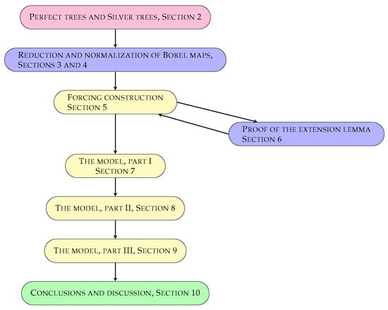
Figure 1. Flowchart of the proof of Theorem 1.

The reader envisaged is assumed to have some knowledge of the pointset topology of the Baire space ${\omega }^{\omega }$ (we give [15] and [1] [Chapter 11] as references) along with some basic knowledge of forcing and Gödel’s constructibility (we give [1,2,16] as references).

2. Silver Trees

The proof of Theorem 1 in this paper will involve a forcing notion $\mathbb{P}$ which consists of Silver trees. Here, we recall the relevant notation.

By $2^{<\omega }$ we denote the set of all tuples (finite sequences) of terms $0,1$, including the empty tuple $\mathsf{\Lambda }$. The length of a tuple s is denoted by $\mathtt{lh}s$, and $2^n=\{s\in 2^{<\omega }:\mathtt{lh}s=n\}$ (all tuples of length n). A tree $⌀\ne T\subseteq 2^{<\omega }$ is a perfect tree, symbolically $T\in \mathbf{PT}$, if it has no endpoints and isolated branches. In this case, the set

$$\left[T\right]=\{a\in 2^{\omega }:\forall n(a\upharpoonright n\in T)\}$$

(2)

of all branches of T is a perfect set in $2^{\omega }.$ If $u\in T\in \mathbf{PT}$, then

$$T{\upharpoonright }_u=\{s\in T:u\subset s\vee s\subseteq u\}\in \mathbf{PT}$$

(3)

is a portion of T. A tree $S\subseteq T$ is clopen in T iff it is equal to the union of a finite number of portions of T. This is equivalent to $\left[S\right]$ being clopen in $\left[T\right]$ as a pointset in $2^{\omega }$.

Definition 1.

A tree $T\in \mathbf{PT}$ is a Silver tree, symbolically $T\in \mathbf{ST}$, if there is an infinite sequence of tuples $u_k=u_k\left(T\right)\in 2^{<\omega },$ such that T consists of all tuples of the form

$$s=u_0\stackrel{⏜}{}{i}_0\stackrel{⏜}{}{u}_1\stackrel{⏜}{}{i}_1\stackrel{⏜}{}{u}_2\stackrel{⏜}{}{i}_2\stackrel{⏜}{}\dots u_n\stackrel{⏜}{}{i}_n$$

and their sub-tuples, where $n<\omega$ and $i_k=0,1$.

Note that the stem $\mathtt{stem}\left(T\right)=u_0\left(T\right)$ of any tree $T\in \mathbf{ST}$ is equal to the largest tuple $s\in T$ with $T=T{\upharpoonright }_s$, and $\left[T\right]$ consists of all infinite sequences $a=u_0\stackrel{⏜}{}{i}_0\stackrel{⏜}{}{u}_1\stackrel{⏜}{}{i}_1\stackrel{⏜}{}{u}_2\stackrel{⏜}{}{i}_2\stackrel{⏜}{}\dots \in 2^{\omega },$ where $i_k=0,1$, $\forall k$. We further put

$${\mathtt{spl}}_n\left(T\right)=\mathtt{lh}{u}_0+1+\mathtt{lh}{u}_1+1+\cdots +\mathtt{lh}{u}_{n-1}+1+\mathtt{lh}{u}_n,$$

(4)

the $n$-th splitting level of a Silver tree T. In particular, ${\mathtt{spl}}_0\left(T\right)=\mathtt{lh}{u}_0$.

Action. Let $\sigma \in 2^{<\omega }.$ If $v\in 2^{<\omega }$ is another tuple of length $\mathtt{lh}v\ge \mathtt{lh}\sigma$, then the tuple $v^{\prime }=\sigma v$ of the same length $\mathtt{lh}{v}^{\prime }=\mathtt{lh}v$ is defined by $v^{\prime }\left(i\right)=v\left(i\right){+}_2\sigma \left(i\right)$ (addition modulo 2) for all $i<\mathtt{lh}\sigma$, but $v^{\prime }\left(i\right)=v\left(i\right)$ whenever $\mathtt{lh}\sigma \le i<\mathtt{lh}v$. If $\mathtt{lh}v<\mathtt{lh}\sigma$, then we just define $\sigma ·v=\left(\sigma \upharpoonright \mathtt{lh}v\right)·v$.

If $a\in 2^{\omega },$ then similarly $a^{\prime }=\sigma a\in 2^{\omega },$ $a^{\prime }\left(i\right)=a\left(i\right){+}_2\sigma \left(i\right)$ for $i<\mathtt{lh}\sigma$, but $a^{\prime }\left(i\right)=a\left(i\right)$ for $i\ge \mathtt{lh}\sigma$. If $T\subseteq 2^{<\omega },X\subseteq 2^{\omega }$, then the sets

$$\sigma T=\{\sigma ·v:v\in T\}\mathrm{and}\sigma ·X=\{\sigma ·a:a\in X\}$$

(5)

are shifts of the tree T and the set X accordingly.

According to (ii) of the next lemma (Lemma 3.4 in [17]), all portions $T{\upharpoonright }_s$, of the same level, of any Silver tree $T\in \mathbf{ST}$ are shifts of each other, or saying it differently, T can be recovered from any its portion. This is not true for arbitrary trees in $\mathbf{PT}$, of course.

Lemma 1.

(i)

If $s\in T\in \mathbf{ST}$ and $\sigma \in 2^{<\omega },$ then $\sigma ·T\in \mathbf{ST}$ and $T{\upharpoonright }_s\in \mathbf{ST}$.

(ii)

If $n<\omega$ and $u,v\in T\cap 2^n,$ then $T{\upharpoonright }_u=v·u·\left(T{\upharpoonright }_v\right)$.

Refinements. Assume that $T,S\in \mathbf{ST}$, $S\subseteq T$, $n<\omega$. We define $S{\subseteq }_{n}T$ (the tree S n-refines T) if $S\subseteq T$ and ${\mathtt{spl}}_k\left(T\right)={\mathtt{spl}}_k\left(S\right)$ for all $k<n$. This is equivalent to ($S\subseteq T$ and) $u_k\left(S\right)=u_k\left(T\right)$ for all $k<n$, of course.

Then, $S{\subseteq }_{0}T$ is equivalent to $S\subseteq T$, and $S{\subseteq }_{n+1}T$ implies $S{\subseteq }_{n}T$ (and $S\subseteq T$).

In addition, if $n\ge 1$ then $S{\subseteq }_{n}T$ is equivalent to ${\mathtt{spl}}_{n-1}\left(T\right)={\mathtt{spl}}_{n-1}\left(S\right)$.

Lemma 2.

Assume that $T,U\in \mathbf{ST},n<\omega ,h>{\mathtt{spl}}_{n-1}\left(T\right),v_0\in 2^h\cap T$, and $U\subseteq T{\upharpoonright }_{v_0}$. Then, there is a unique tree $S\in \mathbf{ST}$ such that $S{\subseteq }_{n}T$ and $S{\upharpoonright }_{v_0}=U.$

If in addition U is clopen in T then S is clopen in T, as well.

Proof. 

Define a tree S so that $S\cap 2^h=T\cap 2^h$, and if $v\in T\cap 2^h$ then, following Lemma 1(ii), $S{\upharpoonright }_v=(v·v_0)·U$; in particular $S{\upharpoonright }_{v_0}=U$. To check that $S\in \mathbf{ST}$, we can easily compute the according tuples $u_k\left(S\right)$ to fulfill Definition 1. Namely, as $U\subseteq T{\upharpoonright }_{v_0}$, we have $v_0\subseteq u_0\left(U\right)=\mathtt{stem}\left(U\right)$, hence the length $\ell =\mathtt{lh}\left(u_0\left(U\right)\right)$ satisfies $\ell \ge h>m={\mathtt{spl}}_{n-1}\left(T\right)$. Then, we have

$$u_k\left(S\right)=\left\{\begin{array}{ccc}\hfill u_k\left(T\right)& \mathrm{for}\mathrm{all}\hfill & k<n,\hfill \\ \hfill u_0\left(U\right)\upharpoonright [m,\ell )& \mathrm{for}\hfill & k=n—\mathrm{thus}{u}_n\left(S\right)\in 2^{\ell -m},\hfill \\ \hfill u_k\left(U\right)& \mathrm{for}\mathrm{all}\hfill & k>n,\hfill \end{array}\right.$$

and Definition 1 for S is satisfied with these tuples $u_k\left(S\right)$. In addition, if U is clopen in T (i.e., U is a finite union of portions in T), then clearly so is S. □

Lemma 3

([17], Lemma 4.4). Let $\dots {\subseteq }_4{T}_3{\subseteq }_3{T}_2{\subseteq }_2{T}_1{\subseteq }_1{T}_0$ be a sequence of trees in $\mathbf{ST}$. Then, $T={\bigcap }_n{t}_n\in \mathbf{ST}$.

Proof 

(sketch). By definition, we have $u_k\left(T_n\right)=u_k\left(T_{n+1}\right)$ for all $k\le n$. Then, one easily computes that $u_n\left(T\right)=u_n\left(T_n\right)$ for all n. □

3. Reduction of Borel Maps to Continuous Ones

A classical theorem claims that in Polish spaces every Borel function is continuous on a suitable dense ${\mathbf{G}}_{\delta }$ set. It is also known that a Borel map defined on $2^{\omega }$ is continuous on a suitable Silver tree. The next lemma combines these two results.

Our interest in Borel functions defined on $2^{\omega }\times {\omega }^{\omega }$ is motivated by further applications to reals in generic extensions of the form $\mathbf{L}[a,x]$, where $a\in 2^{\omega }$ is a $\mathbb{P}$-generic real for a certain forcing notion $\mathbb{P}\subseteq \mathbf{ST}$, whereas $x\in {\omega }^{\omega }$ is just a Cohen generic real. These applications will be based on the fact that any real $y\in 2^{\omega }$ in such an extension can be represented in the form $y=f(a,x)$, where $f:2^{\omega }\times {\omega }^{\omega }\to 2^{\omega }$ is a Borel map coded in the constructible universe $\mathbf{L}$ (Corollary 2 below in Section 5).

In the remainder, if $v\in {\omega }^{<\omega }$ (a tuple of natural numbers), then we define ${\mathcal{N}}_v=\{x\in {\omega }^{\omega }:v\subset x\}$, a clopen Baire interval in the Baire space ${\omega }^{\omega }.$

Lemma 4.

Let $T\in \mathbf{ST}$ and $f:2^{\omega }\times {\omega }^{\omega }\to 2^{\omega }$ be a Borel map. Then, there is a Silver tree $S\subseteq T$ and a dense ${\mathbf{G}}_{\delta }$ set $D\subseteq {\omega }^{\omega }$ such that f is continuous on $\left[S\right]\times D.$

Proof. 

By the abovementioned classical theorem (Theorem 8.38 in Kechris [15]), there exists a dense ${\mathbf{G}}_{\delta }$ set $Z\subseteq \left[T\right]\times {\omega }^{\omega }$ such that f is already continuous on Z. It remains to define a Silver tree $S\subseteq T$ and a dense ${\mathbf{G}}_{\delta }$ set $D\subseteq {\omega }^{\omega }$ such that $\left[S\right]\times D\subseteq Z.$ This will be our goal.

By the choice of Z we have $Z={\bigcap }_n{Z}_n$, where each $Z_n\subseteq \left[T\right]\times {\omega }^{\omega }$ is open dense.

Let us fix an enumeration $\omega \times {\omega }^{<\omega }=\{⟨N_k,v_k⟩:k<\omega \}$ of the cartesian product $\omega \times {\omega }^{<\omega }.$ We shall define a sequence of Silver trees $S_k$ and tuples $w_k\in {\omega }^{<\omega }$ satisfying the following three conditions (a)–(c):

(a)

$\dots {\subseteq }_4{S}_3{\subseteq }_3{S}_2{\subseteq }_2{s}_1{\subseteq }_1{S}_0=T$, as in Lemma 3;

(b)

if $k<\omega$ then $S_{k+1}$ is clopen in $S_k$ (see Section 2);

(c)

$v_k\subseteq w_k$ and $\left[S_{k+1}\right]\times {\mathcal{N}}_{w_k}\subseteq Z_{N_k}$, for all k.

At step 0 we already have $S_0=T$ by (a).

Assume that a tree $S_k\in \mathbf{ST}$ has already been defined. Let $h={\mathtt{spl}}_{k+1}\left(S_k\right)$.

Consider any tuple $t\in 2^h\cap S_k.$ As $Z_{N_k}$ is open dense, there is a tuple $u_1\in {\omega }^{<\omega }$ and a Silver tree $A_1\subseteq S_k{\upharpoonright }_t$, clopen in $S_k$ (for example, a portion in $S_k$) such that $v_k\subseteq u_1$ and $\left[A_1\right]\times {\mathcal{N}}_{u_1}\subseteq Z_{N_k}$. According to Lemma 2, there exists a Silver tree $U_1{\subseteq }_{k+1}{S}_k$, clopen in $S_k$ along with A, such that $U_1{\upharpoonright }_t=A_1$, so $\left[U_1{\upharpoonright }_t\right]\times {\mathcal{N}}_{u_1}\subseteq Z_{N_k}$ by construction.

Now, take another tuple $t^{\prime }\in 2^h\cap S_k,$ and similarly find $u_2\in {\omega }^{<\omega }$ and a Silver tree $A_2\subseteq U_1{\upharpoonright }_{t^{\prime }}$, clopen in $U_1$, such that $u_1\subseteq u_2$ and $\left[A_2\right]\times {\mathcal{N}}_{u_2}\subseteq Z_{N_k}$. Once again, there is a Silver tree $U_2{\subseteq }_{k+1}{U}_1$, clopen in $S_k$ and such that $\left[U_2{\upharpoonright }_{t^{\prime }}\right]\times {\mathcal{N}}_{u_2}\subseteq Z_{N_k}$.

We iterate this construction over all tuples $t\in 2^h\cap S_k,$ ${\subseteq }_{k+1}$-shrinking trees and extending tuples in ${\omega }^{<\omega }.$ We obtain a Silver tree $U{\subseteq }_{k+1}{S}_k$, clopen in $S_k$, and a tuple $w\in {\omega }^{<\omega },$ that $v_k\subseteq w$ and $\left[U\right]\times {\mathcal{N}}_w\subseteq Z_{N_k}$. Take $w_k=w,S_{k+1}=U$. This completes the inductive step.

As a result we obtain a sequence $\dots {\subseteq }_4{S}_3{\subseteq }_3{S}_2{\subseteq }_2{S}_1{\subseteq }_1{S}_0=T$ of Silver trees $S_k$, and tuples $w_k\in {\omega }^{<\omega }$ ($k<\omega$), which really satisfy conditions (a)–(c).

We put $S={\bigcap }_k{S}_k$; then $S\in \mathbf{ST}$ by (a) and Lemma 3, and $S\subseteq T$.

If $n<\omega$ then let $W_n=\{w_k:N_k=n\}$. We claim that $D_n={\bigcup }_{w\in W_n}{\mathcal{N}}_w$ is an open dense set in ${\omega }^{\omega }.$ Indeed, let $v\in {\omega }^{<\omega }.$ Consider any k such that that $v_k=v$ and $N_k=n$. By construction, we have $v\subseteq w_k\in W_n$. Thus the set $D={\bigcap }_n{D}_n$ is dense and ${\mathbf{G}}_{\delta }$.

To check $\left[S\right]\times D\subseteq Z$, let $n<\omega$; we show that $\left[S\right]\times D\subseteq Z_n$. Let $a\in \left[S\right]$ and $x\in D$, in particular $x\in D_n$, so $x\in {\mathcal{N}}_{w_k}$ for some k with $N_k=n$. However, $\left[S_{k+1}\right]\times {\mathcal{N}}_{w_k}\subseteq Z_n$ by (c), and at the same time obviously $a\in \left[S_{k+1}\right]$. Therefore, $⟨a,x⟩\in Z_n$, as required. □

Corollary 1.

Suppose that $T\in \mathbf{ST}$ and $f:2^{\omega }\to 2^{\omega }$ be a Borel map. Then there is a Silver tree $S\subseteq T$ such that f is continuous on $\left[S\right].$

We add the following result that belongs to the folklore of the Silver forcing. See Corollary 5.4 in [18] for a proof.

Lemma 5.

Assume that $T\in \mathbf{ST}$ and $f:2^{\omega }\to 2^{\omega }$ is a continuous map. Then there is a Silver tree $S\subseteq T$ such that f is either a bijection or a constant on $\left[S\right]$.

4. Normalization of Borel Maps

In this section, we continue studying the behavior of Borel maps defined on $2^{\omega }\times {\omega }^{\omega }$ modulo restrictions on products of Silver trees and dense ${\mathbf{G}}_{\delta }$ sets. We work in the context of the following definition of normalization, and the following Lemma 6 will be of key importance in the applications to the genetic extensions below in Section 6.

Definition 2.

A map $f:2^{\omega }\times {\omega }^{\omega }\to 2^{\omega }$ is normalized on a tree $T\in \mathbf{ST}$ for a set of trees $\mathbb{U}\subseteq \mathbf{ST}$ if there exists a dense ${\mathbf{G}}_{\delta }$ set $X\subseteq {\omega }^{\omega }$ such that f is continuous on $\left[T\right]\times X$ and

−

either(I)there are tuples $v\in {\omega }^{<\omega },\sigma \in 2^{<\omega }$ such that $f(a,x)=\sigma ·a$ for all $a\in \left[T\right]$ and $x\in {\mathcal{N}}_v\cap X$, where, we remind, ${\mathcal{N}}_v=\{x\in {\omega }^{\omega }:v\subset x\};$

−

or(II)$f(a,x)\notin {\bigcup }_{\sigma \in 2^{<\omega }\wedge S\in \mathbb{U}}\sigma ·\left[S\right]$ for all $a\in \left[T\right]$ and $x\in X.$

Lemma 6.

Assume that $\mathbb{U}=\{T_0,T_1,T_2,\dots \}\subseteq \mathbf{ST}$ and $f:2^{\omega }\times {\omega }^{\omega }\to 2^{\omega }$ is a Borel map. Then there exists a set of trees ${\mathbb{U}}^{\prime }=\{S_0,S_1,S_2,\dots \}\subseteq \mathbf{ST}$, such that $S_n\subseteq T_n$ for all n and f is normalized on $S_0$ for ${\mathbb{U}}^{\prime }$.

Proof. 

First of all, according to Lemma 4, there is a Silver tree $T^{\prime }\subseteq T_0$ and a dense ${\mathbf{G}}_{\delta }$ set $W\subseteq {\omega }^{\omega }$ such that f is continuous on $\left[T^{\prime }\right]\times W$. Since any dense ${\mathbf{G}}_{\delta }$ set $X\subseteq {\omega }^{\omega }$ is homeomorphic to ${\omega }^{\omega },$ we can w.l.o.g. assume that $W={\omega }^{\omega }$ and $T^{\prime }=T_0$. In other words, we just suppose that f is already continuous on $\left[T_0\right]\times {\omega }^{\omega }.$

Assume that option (I) of Definition 2 does not take place, that is

(∗)

if $X\subseteq {\omega }^{\omega }$ is a dense ${\mathbf{G}}_{\delta }$ set, and $v\in {\omega }^{<\omega },\sigma \in 2^{<\omega },S\in \mathbf{ST},S\subseteq T_0$, then there exist reals $a\in \left[S\right]$ and $x\in {\mathcal{N}}_v\cap X$ such that $f(a,x)\ne \sigma ·a$.

We shall construct Silver trees $S_n\subseteq T_n$ and a dense ${\mathbf{G}}_{\delta }$ set $X\subseteq {\omega }^{\omega }$ satisfying (II) of Definition 2, that is, in our context, the negative relation $f(a,x)\notin {\bigcup }_{\sigma \in 2^{<\omega }\wedge n<\omega }\sigma ·\left[S_n\right]$ will be fulfilled for all $a\in \left[S_0\right]$ and $x\in X.$ To maintain the construction, let us fix an arbitrary enumeration

$$\omega \times 2^{<\omega }\times {\omega }^{<\omega }=\{⟨N_k,{\sigma }_k,v_k⟩:k<\omega \}.$$

(6)

Further, auxiliary Silver trees $S_k^n$ ($n,k<\omega$) and tuples $w_k\in {\omega }^{<\omega }$ ($k<\omega$) will be defined, satisfying the following conditions (a)–(c).

(a)

$\dots {\subseteq }_4{S}_3^n{\subseteq }_3{S}_2^n{\subseteq }_2{S}_1^n{\subseteq }_1{S}_0^n=T_n$ as in Lemma 3, for each $n<\omega$;

(b)

$S_{k+1}^n=S_k^n$ for all $n>0,n\ne N_k$;

(c)

$S_{k+1}^0{\subseteq }_{k+1}{S}_k^0$, $S_{k+1}^{N_k}{\subseteq }_{k+1}{S}_k^{N_k}$, $v_k\subseteq w_k$, and $f(a,x)\notin {\sigma }_k·\left[S_{k+1}^N\right]$ for all reals $a\in \left[S_{k+1}^0\right]$ and $x\in {\mathcal{N}}_{w_k}$.

At step 0 of the construction, we input $S_0^n=T_n$ for all n, according to (a).

Assume that $k<\omega$ and all Silver trees $S_k^n,n<\omega$ are already defined. We input $S_{k+1}^n=S_k^n$ for all $n>0,n\ne N_k$, by (b). (The number $N_k$ is defined by (6).)

To define the trees $S_{k+1}^0$ and $S_{k+1}^{N_k}$, we put $h={\mathtt{spl}}_{k+1}\left(S_k^0\right)$, $m={\mathtt{spl}}_{k+1}\left(S_k^N\right)$.

Case 1: $N_k>0$. Take any pair of tuples $s\in 2^h\cap S_k^0$, $t\in 2^m\cap S_k^{N_k}$ and any reals $a_0\in \left[S_k^0{\upharpoonright }_s\right]$ and $x_0\in {\omega }^{\omega }.$ Consider any real $b_0\in \left[S_k^{N_k}{\upharpoonright }_t\right]$ not equal to ${\sigma }_k·f(a_0,x_0)$. Let us say $b_0(\ell )=i\ne j=({\sigma }_k·f(a_0,x_0))(\ell )$, where $i,j\le 1,\ell <\omega$. As f is continuous, there is a tuple $u_1\in {\omega }^{<\omega }$ and a Silver tree $A\subseteq S_k^0{\upharpoonright }_s$ such that $v_k\subseteq u_1\subset x_0$, $a_0\in \left[A\right]$, and $({\sigma }_k·f(a,x))(\ell )=j$ for all $x\in {\mathcal{N}}_{u_1}$ and $a\in \left[A\right]$. It is also clear that

$$B=\{\tau \in S_k^{N_k}{\upharpoonright }_t:\mathtt{lh}\tau \le \ell \vee \tau (\ell )=i\}$$

(7)

is a Silver tree containing $b_0$, and $b(\ell )=i$ for all $b\in \left[B\right]$. According to Lemma 2, there exist Silver trees $U_1{\subseteq }_{k+1}{S}_k^0$ and $V_1{\subseteq }_{k+1}{S}_k^{N_k}$, such that $U_1{\upharpoonright }_s=A$ and $V_1{\upharpoonright }_t=B$. It follows by construction that ${\sigma }_k·f(a,x)\notin \left[V_1{\upharpoonright }_t\right]$ for all $a\in \left[U_1{\upharpoonright }_s\right]$ and $x\in {\mathcal{N}}_{u_1}$.

Now, consider another pair of tuples $s^{\prime }\in 2^h\cap S_k^0$, $t^{\prime }\in 2^m\cap S_k^{N_k}$. We similarly obtain Silver trees $U_2{\subseteq }_{k+1}{U}_1$ and $V_2{\subseteq }_{k+1}{V}_1$, and a tuple $u_2\in {\omega }^{<\omega },$ such that $u_1\subseteq u_2$ and ${\sigma }_k·f(a,x)\notin \left[V_2\left(\to t^{\prime }\right)\right]$ for all $a\in \left[U_2{\upharpoonright }_{s^{\prime }}\right]$ and $x\in {\mathcal{N}}_{u_2}$. In this case, we have $V_2{\upharpoonright }_t\subseteq V_1{\upharpoonright }_t$ and $U_2{\upharpoonright }_s\subseteq U_1{\upharpoonright }_s$, so that what has already been achieved in the previous step $(s,t)$ is preserved.

We iterate over all pairs of $s\in 2^h\cap S_k^0$, $t\in 2^m\cap S_k^{N_k}$, by ${\subseteq }_{k+1}$-shrinking trees and extending tuples in ${\omega }^{<\omega }$ at each step. This results in a pair of Silver trees $U{\subseteq }_{k+1}{S}_k^0,V{\subseteq }_{k+1}{S}_k^{N_k}$ and a tuple $w\in {\omega }^{<\omega }$ such that $v_k\subseteq w$ and ${\sigma }_{k}f(a,x)\notin \left[V\right]$ for all reals $a\in \left[U\right]$ and $x\in {\mathcal{N}}_w$. Now, to fulfill (c), take $w_k=w$, $S_{k+1}^0=U,$ and $S_{k+1}^{N_k}=V.$ Recall that here $N_k>0$.

Case 2: $N_k=0$. Here, the construction somewhat changes, and hypothesis (∗) will be used. We claim that there exist:

(d)

a tuple $w_k\in {\omega }^{<\omega }$ and a Silver tree $S_{k+1}^0{\subseteq }_{k+1}{S}_k^0$ such that $v_k\subseteq w_k$ and $f(a,x)\notin {\sigma }_k\begin{array}{c}\hfill (0,1)(0,-3)*2.1\end{array}\left[S_{k+1}^0\right]$ for all $a\in \left[S_{k+1}^0\right]$, $x\in {\mathcal{N}}_{w_k}$. (This is equivalent to (c) as $N_k=0$.)

Take any pair of tuples $s,t\in 2^h\cap S_k^0$, where $h={\mathtt{spl}}_{k+1}\left(S_k^0\right)$ as above. Thus, $S_k^0{\upharpoonright }_t=ts\left(S_k^0{\upharpoonright }_s\right)$, by Lemma 1(ii). According to (∗), there are reals $x_0\in {\mathcal{N}}_v$ and $a_0\in \left[S_k^0{\upharpoonright }_s\right]$ satisfying $f(a_0,x_0)\ne {\sigma }_k·s·t·a_0$, or equivalently, ${\sigma }_k·f(a_0,x_0)\ne s·t·a_0$.

Similarly to Case 1, we have $({\sigma }_k·f(a_0,x_0))(\ell )=i\ne j=(s·t·a_0)(\ell )$ for some $\ell <\omega$ and $i,j\le 1$. By the continuity of f, there is a tuple $u_1\in {\omega }^{<\omega }$ and a Silver tree $A\subseteq S_k^0{\upharpoonright }_s$, clopen in $S_k^0$, such that $v_k\subseteq u_1\subset x_0$, $a_0\in \left[A\right]$, and $({\sigma }_k·f(a,x))(\ell )=j$ but $(s·t·a)(\ell )=j$ for all $x\in {\mathcal{N}}_{u_1}$ and $a\in \left[A\right]$. Lemma 2 gives us a Silver tree $U_1{\subseteq }_{k+1}{S}_k^0$, clopen in $S_k^0$ as well, such that $U_1{\upharpoonright }_s=A$ — and then $U_1{\upharpoonright }_t=s·t·A$. Therefore, ${\sigma }_k·f(a,x)\notin \left[U_1{\upharpoonright }_t\right]$ holds for all $a\in \left[U_1{\upharpoonright }_s\right]$ and $x\in {\mathcal{N}}_{u_1}$ by construction.

Having considered all pairs of tuples $s,t\in 2^h\cap S_k^0$, we obtain a Silver tree $U{\subseteq }_{k+1}{S}_k^0$ and a tuple $w\in {\omega }^{<\omega },$ such that $v_k\subseteq w$ and ${\sigma }_k·f(a,x)\notin \left[U\right]$ for all $a\in \left[U\right]$ and $x\in {\mathcal{N}}_w$. Now, to fulfill (d), take $w_k=w$ and $S_{k+1}^0=U$. This concludes Case 2.

To conclude, we have for each n a sequence $\dots {\subseteq }_4{S}_3^n{\subseteq }_3{S}_2^n{\subseteq }_2{S}_1^n{\subseteq }_1{S}_0^n=T_n$ of Silver trees $S_k^n$, along with tuples $w_k\in {\omega }^{<\omega }$ ($k<\omega$), and these sequences satisfy the requirements (a)–(c) (equivalent to (d) in case $N_k=0$).

We put $S_n={\bigcap }_k{S}_k^n$ for all n. Then, $S_n\in \mathbf{ST}$ by Lemma 3, and $S_n\subseteq T_n$.

If $n<\omega$ and $\sigma \in 2^{<\omega }$, then let $W_{n\sigma }=\{w_k:N_k=n\wedge {\sigma }_k=\sigma \}$. The set $X_{n\sigma }={\bigcup }_{w\in W_{n\sigma }}{\mathcal{N}}_w$ is then open dense in ${\omega }^{\omega }.$ Indeed, if $v\in {\omega }^{\omega }$, then we take k such that $v_k=v,N_k=n,{\sigma }_k=\sigma$; then $v\subseteq w_k\in W_{n\sigma }$ by construction. Therefore, $X={\bigcap }_{n<\omega ,\sigma \in 2^{<\omega }}{X}_{n\sigma }$ is a dense ${\mathbf{G}}_{\delta }$ set. Now, to check property (II) of Definition 2, consider any $n<\omega ,\sigma \in 2^{<\omega },a\in \left[S_0\right],x\in X$; we claim that $f(a,x)\notin \sigma ·\left[S_n\right]$.

Indeed, by construction we have $x\in X_{n\sigma }$, i.e., $x\in {\mathcal{N}}_{w_k}$, where $k\in W_{n\sigma }$, so that $N_k=n,{\sigma }_k=\sigma$. Now, $f(a,x)\notin \sigma \left[S_n\right]$ directly follows from (c) for this k, since $S_0\subseteq S_{k+1}^0$ and $S_n\subseteq S_{k+1}^n$. □

5. The Forcing Notion for Theorem 1

In this section, we define a forcing notion $\mathbb{P}\in \mathbf{L}$, $\mathbb{P}\subseteq \mathbf{ST}$, involved in the proof of Theorem 1. This will be a rather lengthy construction, and we begin with auxiliary material.

We use letters ${\Sigma }_{}^{}$ and ${\Pi }_{}^{}$ to denote effective (lightface) projective classes.

Using the standard encoding of Borel sets, as e.g., in [19], or [20] [§ 1D], we make use of coding systems for Borel functions $f:2^{\omega }\times {\omega }^{\omega }\to 2^{\omega }$ and $g:2^{\omega }\to 2^{\omega }.$

(A)

We fix a coding system for Borel functions $g:2^{\omega }\to 2^{\omega },$ which includes a ${\Pi }_1^1$-set of codes $\mathbf{BC}\subseteq {\omega }^{\omega }$, and for each code $r\in \mathbf{BC}$, a certain Borel function $F_r:2^{\omega }\to 2^{\omega }$ coded by $r.$ We assume that each Borel function has some code, and there is a ${\Sigma }_1^1$ relation $\mathfrak{S}(·,·,·)$ and a ${\Pi }_1^1$ relation $\mathfrak{P}(·,·,·)$ such that for all $r\in \mathbf{BC}$ and $a,b\in 2^{\omega }$ it holds $F_r\left(a\right)=b⟺\mathfrak{S}(r,a,b)⟺\mathfrak{P}(r,a,b)$.

(B)

We fix a coding system for Borel functions $f:2^{\omega }\times {\omega }^{\omega }\to 2^{\omega },$ that includes a ${\Pi }_1^1$-set of codes ${\mathbf{BC}}_{\mathbf{2}}\subseteq {\omega }^{\omega }$, and for each code $r\in {\mathbf{BC}}_{\mathbf{2}}$, a Borel function $F_r^2:2^{\omega }\times {\omega }^{\omega }\to 2^{\omega }$ coded by r, such that each Borel function has some code, and there is a ${\Sigma }_1^1$ relation ${\mathfrak{S}}^2(·,·,·,·)$ and a ${\Pi }_1^1$ relation ${\mathfrak{P}}^2(·,·,·,·)$ such that for all $r\in {\mathbf{BC}}_{\mathbf{2}},x\in {\omega }^{\omega },$ and $a,b\in 2^{\omega }$ it holds $F_r^2(a,x)=b⟺{\mathfrak{S}}^2(r,a,x,b)⟺{\mathfrak{P}}^2(r,a,x,b)$.

If $\mathbb{U}\subseteq \mathbf{ST}$, then $\mathbf{Clos}\left(\mathbb{U}\right)$ denotes the set of all trees of the form $\sigma ·\left(T{\upharpoonright }_s\right)$, where $\sigma \in 2^{<\omega }$ and $s\in T\in \mathbb{U}$, i.e., the closure of $\mathbb{U}$ w.r.t. both shifts and portions.

The following construction is maintained in $\mathbf{L}$. We define a sequence of countable sets ${\mathbb{U}}_{\alpha }\subseteq \mathbf{ST},\alpha <{\omega }_1$ satisfying the following conditions 1°–6°.

1°

Each ${\mathbb{U}}_{\alpha }\subseteq \mathbf{ST}$ is countable, ${\mathbb{U}}_0$ consists of a single tree $2^{<\omega }.$

We then define ${\mathbb{P}}_{\alpha }=\mathbf{Clos}\left({\mathbb{U}}_{\alpha }\right)$, ${\mathbb{P}}_{<\alpha }={\bigcup }_{\xi <\alpha }{\mathbb{P}}_{\xi }$. These sets are obviously closed with respect to shifts and portions, that is, $\mathbf{Clos}\left({\mathbb{P}}_{\alpha }\right)={\mathbb{P}}_{\alpha }$ and $\mathbf{Clos}\left({\mathbb{P}}_{<\alpha }\right)={\mathbb{P}}_{<\alpha }$.

2°

For every $T\in {\mathbb{P}}_{<\alpha }$, there is a tree $S\in {\mathbb{U}}_{\alpha },S\subseteq T$.

Let ${\mathbf{ZFC}}^{-}$ be the sub-theory of ZFC, containing all axioms except the power set axiom (and with the wellorderability principle instead of AC), and additionally containing an axiom asserting the existence of the power set $\mathcal{P}\left(\omega \right)$. This implies the existence of $\mathcal{P}\left(X\right)$ for any countable X, the existence of ${\omega }_1$ and $2^{\omega }$, as well as the existence of continual sets like $2^{\omega }$ or $\mathbf{ST}$.

By ${\mathfrak{M}}_{\alpha }$ we denote the smallest model of ${\mathbf{ZFC}}^{-}$ of the form ${\mathbf{L}}_{\lambda }$ containing the sequence ${⟨{\mathbb{U}}_{\xi }⟩}_{\xi <\alpha }$, in which $\alpha$ and all sets ${\mathbb{U}}_{\xi },\xi <\alpha$ are countable.

3°

If a set $D\in {\mathfrak{M}}_{\alpha },D\subseteq {\mathbb{P}}_{<\alpha }$ is dense in ${\mathbb{P}}_{<\alpha }$, and $U\in {\mathbb{U}}_{\alpha }$, then $U{\subseteq }^{\mathrm{fin}}\bigcup D$, meaning that there is a finite set $D^{\prime }\subseteq D$ such that $U\subseteq \bigcup D^{\prime }$.

4°

If a set $D\in {\mathfrak{M}}_{\alpha },D\subseteq {\mathbb{P}}_{<\alpha }\times {\mathbb{P}}_{<\alpha }$ is dense in ${\mathbb{P}}_{<\alpha }\times {\mathbb{P}}_{<\alpha }$, and $U\ne V$ belong to ${\mathbb{U}}_{\alpha }$, then $U\times V{\subseteq }^{\mathrm{fin}}\bigcup D$, meaning that there is a finite set $D^{\prime }\subseteq D$ such that $\left[U\right]\times \left[V\right]\subseteq {\bigcup }_{⟨U^{\prime },V^{\prime }⟩\in D^{\prime }}\left[U^{\prime }\right]\times \left[V^{\prime }\right]$.

Given that $\mathbf{Clos}\left({\mathbb{P}}_{<\alpha }\right)={\mathbb{P}}_{<\alpha }$, this is automatically transferred to all trees $U\in {\mathbb{P}}_{\alpha }$, as well. It follows that D remains pre-dense in ${\mathbb{P}}_{<\alpha }\cup {\mathbb{P}}_{\alpha }$.

To formulate the next property, we fix an enumeration

$$\mathbf{ST}\times \mathbf{BC}\times {\mathbf{BC}}_{\mathbf{2}}=\{⟨T_{\xi },b_{\xi },c_{\xi }⟩:\xi <{\omega }_1\}$$

(8)

in $\mathbf{L}$, which (1) is definable in ${\mathbf{L}}_{{\omega }_1}$, and (2) involves each value in $\mathbf{ST}\times \mathbf{BC}\times {\mathbf{BC}}_{\mathbf{2}}$ being taken uncountably many times.

5°

If $T_{\alpha }\in {\mathbb{P}}_{<\alpha }$, then there is a tree $S\in {\mathbb{U}}_{\alpha }$ such that $S\subseteq T$ and:

• $F_{b_{\alpha }}^2$ is normalized for ${\mathbb{U}}_{\alpha }$ on $\left[S\right]$ in the sense of Definition 2, and
• $F_{c_{\alpha }}$ is continuous and either a bijection or a constant on $\left[S\right]$.

6°

The sequence ${⟨{\mathbb{U}}_{\alpha }⟩}_{\alpha <{\omega }_1}$ is $\in$-definable in ${\mathbf{L}}_{{\omega }_1}$.

The construction 1°–6° goes on as follows. We work in $\mathbf{L}$.

We first define ${\mathbb{U}}_0=\left\{2^{<\omega }\right\},$ to obey 1°.

Now, suppose that

(†)

$0<\alpha <{\omega }_1$, the subsequence ${⟨{\mathbb{U}}_{\xi }⟩}_{\xi <\alpha }$ is defined and satisfies 1°, 2° below $\alpha$, and the sets ${\mathbb{P}}_{\xi }=\mathbf{Clos}\left({\mathbb{U}}_{\xi }\right)$ (for $\xi <\alpha$), ${\mathbb{P}}_{<\alpha }$, ${\mathfrak{M}}_{\alpha }$ are defined as above.

The induction step of the construction is based on the following lemma.

Lemma 7

(in $\mathbf{L}$, see the proof in Section 6). Under the assumptions of (†), there is a countable set ${\mathbb{U}}_{\alpha }\subseteq \mathbf{ST}$ satisfying conditions 2°, 3°, 4°, 5°.

To accomplish the construction on the base of the lemma, we take ${\mathbb{U}}_{\alpha }$ to be the smallest, in the sense of the Gödel wellordering of $\mathbf{L}$, of those sets that exist by Lemma 7. Since the whole construction is relativized to ${\mathbf{L}}_{{\omega }_1}$, requirement 6° is also met.

We put ${\mathbb{P}}_{\alpha }=\mathbf{Clos}\left({\mathbb{U}}_{\alpha }\right)$ for all $\alpha <{\omega }_1$, and $\mathbb{P}={\bigcup }_{\alpha <{\omega }_1}{\mathbb{P}}_{\alpha }$.

The next result, in part related to the countable chain condition, or CCC for brevity, is a fairly standard consequence of 3° and 4°, see for example [13] (6.5), [18] (12.4), or [21] (Lemma 6); we will omit the proof. Recall that a forcing notion $\mathbb{Q}$ satisfies CCC iff every antichain $A\subseteq \mathbb{Q}$ is finite or countable.

Lemma 8

(in $\mathbf{L}$). The forcing notion $\mathbb{P}$ belongs to $\mathbf{L}$, satisfies $\mathbb{P}=\mathbf{Clos}\left(\mathbb{P}\right)$ and satisfies CCC in $\mathbf{L}$. The product $\mathbb{P}\times \mathbb{P}$ satisfies CCC in $\mathbf{L}$, as well.

Corollary 2.

(i)

If a real $a\in 2^{\omega }$ is $\mathbb{P}$-generic over $\mathbf{L}$ and $y\in 2^{\omega }\cap \mathbf{L}\left[a\right]$, then there is a Borel map $g=F_b:2^{\omega }\to 2^{\omega }$ with a code $b\in \mathbf{L}\cap \mathbf{BC}$ such that $y=f\left(a\right)$.

(ii)

If a pair $⟨a,x⟩\in 2^{\omega }\times {\omega }^{\omega }$ is $(\mathbb{P}\times \mathbb{C})$-generic over $\mathbf{L}$ and $y\in 2^{\omega }\cap \mathbf{L}[a,x]$ then there is a Borel map $f=F_b^2:2^{\omega }\times {\omega }^{\omega }\to 2^{\omega }$ with a code $b\in \mathbf{L}\cap {\mathbf{BC}}_{\mathbf{2}}$ such that $y=f(a,x)$.

Proof. (i)

By the Gödel constructibility theory, there is an ordinal $\xi <{\omega }_1^{\mathbf{L}\left[a\right]}$ such that y is the $\xi$th element of $\mathbf{L}\left[a\right]\cap 2^{\omega }$ in the sense of the canonical wellordering of $\mathbf{L}\left[a\right]$. However, the forcing notion $\mathbb{P}$ preserves cardinals by Lemma 8, and hence $\xi <{\omega }_1^{\mathbf{L}}={\omega }_1^{\mathbf{L}\left[a\right]}$. Finally, as $\xi <{\omega }_1^{\mathbf{L}}$, it is known that the map

$$a⟼\left(\mathrm{the}\xi \mathrm{th}\mathrm{element}\mathrm{of}\mathbf{L}\left[a\right]\cap 2^{\omega }\right)$$

(9)

is ${\Delta }_1^1\left(p\right)$ with a parameter $p\in \mathbf{L}\cap 2^{\omega }$ by [20], Theorem 2.6(ii), and, hence, the map (9) is Borel with a code in $\mathbf{L}$, as required.

The proof of (ii) is similar. The forcing notion $\mathbb{P}\times \mathbb{C}$ satisfies CCC since so does $\mathbb{P}$, whereas $\mathbb{C}$ is countable. □

Lemma 9

(in $\mathbf{L}$). Assume that $T\in \mathbb{P}$. If $g:2^{\omega }\to 2^{\omega }$ is a Borel map then there is a tree $S\in {\mathbb{U}}_{\alpha }$, $S\subseteq T$, such that g is either a bijection or a constant on $\left[S\right]$.

If $f:2^{\omega }\times {\omega }^{\omega }\to 2^{\omega }$ is a Borel map, then there is an ordinal $\alpha <{\omega }_1$ and a tree $S\in {\mathbb{U}}_{\alpha }$, $S\subseteq T$, such that f is normalized for ${\mathbb{U}}_{\alpha }$ on $\left[S\right]$.

Proof. 

By the choice of the enumeration (8) of triples in $\mathbf{ST}\times \mathbf{BC}\times {\mathbf{BC}}_{\mathbf{2}},$ there is an ordinal $\alpha <{\omega }_1$ such that $T\in {\mathbb{P}}_{<\alpha }$ and $T=T_{\alpha }$, $f=F_{b_{\alpha }}^2$, $g=F_{b_{\alpha }}$. Now, we refer to 5°. □

6. Proof of the Extension Lemma

Proof 

(proof of Lemma 7). This section is entirely devoted to the proof of Lemma 7.

We work in $\mathbf{L}$ under the assumptions of (†) above.

We first define a set $\mathbb{U}=\{U_n:n<\omega \}$ of Silver trees $U_n\subseteq 2^{\omega }$ satisfying 2°, 3° 4° then further narrowing of the trees will be performed to also satisfy 5°. This involves a splitting/fusion construction known from our earlier papers, see [13] (§ 4), [17] (§ 9–10), [18] (§ 10), and to some extent from the proof of Lemma 6 above.

We fix a bijection $\beta :\omega \stackrel{\mathrm{onto}}{⟶}{\omega }^4$. We also fix enumerations

$$\mathcal{D}=\{D\left(j\right):j<\omega \}\mathrm{and}{\mathcal{D}}_2=\{D_2\left(j\right):j<\omega \}$$

(10)

of the set $\mathcal{D}$ of all sets $D\in {\mathfrak{M}}_{\alpha },D\subseteq {\mathbb{P}}_{<\alpha }$ open dense in ${\mathbb{P}}_{<\alpha }$, and the set ${\mathcal{D}}_2$ of all sets $D\in {\mathfrak{M}}_{\alpha },D\subseteq {\mathbb{P}}_{<\alpha }\times {\mathbb{P}}_{<\alpha }$ open dense in ${\mathbb{P}}_{<\alpha }\times {\mathbb{P}}_{<\alpha }$.

The construction of the trees $U_n$ is organized in the form $U_n={\bigcup }_k{U}_k^n$, where the Silver trees $U_k^n$ satisfy the following requirements (a)–(d):

(a)

We have $\dots {\subseteq }_4{U}_3^n{\subseteq }_3{U}_2^n{\subseteq }_2{U}_1^n{\subseteq }_1{U}_0^n$ as in Lemma 3 for each $n<\omega$;

(b)

if $T\in {\mathbb{P}}_{<\alpha }$ then $T=U_0^n$ for some n;

(c)

each $U_k^n$ is a $k$-collage over ${\mathbb{P}}_{<\alpha }$.

Here, a Silver tree T is a $k$-collage over ${\mathbb{P}}_{<\alpha }$ [17,18] when $T{\upharpoonright }_s\in {\mathbb{P}}_{<\alpha }$ for each tuple $s\in T\cap 2^h,$ where $h={\mathtt{spl}}_k\left(T\right)$. Then 0-collages are just trees in ${\mathbb{P}}_{<\alpha }$, and every $k$-collage is a $k+1$-collage as well, since $\mathbf{Clos}\left({\mathbb{P}}_{<\alpha }\right)={\mathbb{P}}_{<\alpha }$.

(d)

If $k\ge 1$, $\beta \left(k\right)=⟨j,j^{\prime },M,N⟩$, $\mu ={\mathtt{spl}}_k\left(U_k^M\right)$, $\nu ={\mathtt{spl}}_k\left(U_k^N\right)$ (integers), $s\in U_k^M\cap 2^{\mu }$, $t\in U_k^N\cap 2^{\nu }$ (tuples of length, resp., $\mu ,\nu$), $M\ne N$, then the tree $U_k^M{\upharpoonright }_s$ belongs to $D\left(j\right)$ and the pair $⟨U_k^M{\upharpoonright }_s,U_k^N{\upharpoonright }_t⟩$ belongs to $D_2\left(j^{\prime }\right)$. — It follows that $U_k^M{\subseteq }^{\mathrm{fin}}\bigcup D\left(j\right)$ and $⟨U_k^M,U_k^N⟩{\subseteq }^{\mathrm{fin}}\bigcup D_2\left(j^{\prime }\right)$ in the sense of 3°, 4° of Section 5.

To begin the inductive construction of the trees $U_k^n$, we assign $U_0^n\in {\mathbb{P}}_{<\alpha }$ so that $\{U_0^n:n<\omega \}={\mathbb{P}}_{<\alpha }$, to obtain (b). Now, let us maintain the step $k\to k+1$; it continues simultaneously for all n. Thus, suppose that $k<\omega$, and all Silver trees $U_k^n,n<\omega$ are defined and are $k$-collages over ${\mathbb{P}}_{<\alpha }$.

Let $\beta \left(k\right)=⟨j,j^{\prime },M,N⟩$. If $N=M$, then put $U_{k+1}^n=U_k^n$ for all n.

Now, assume that $M\ne N.$ Put $U_{k+1}^n=U_k^n$ for all $n\notin \{M,N\}$.

It takes more effort to define $U_{k+1}^M$ and $U_{k+1}^N$. Let $\mu ={\mathtt{spl}}_{k+1}\left(U_k^M\right)$, $\nu ={\mathtt{spl}}_{k+1}\left(U_k^N\right)$. To begin with, we input $U_{k+1}^M:=U_k^M$ and $U_{k+1}^N:=U_k^N$. These $k+1$-collages are the initial values for the trees $U_{k+1}^M$ and $U_{k+1}^N$, to be ${\subseteq }_{k+1}$-shrunk in a finite number of substeps (within the step $k\to k+1$), each substep corresponding to a pair of tuples $s\in U_k^M\cap 2^{\mu }$ and $t\in U_k^N\cap 2^{\nu }$.

Namely, let $s\in U_{k+1}^M\cap 2^{\mu }$, $t\in U_{k+1}^N\cap 2^{\nu }$ be the first such pair. The trees $U_{k+1}^M{\upharpoonright }_s$, $U_{k+1}^N{\upharpoonright }_t$ belong to ${\mathbb{P}}_{<\alpha }$ as $U_{k+1}^M$, $U_{k+1}^N$ are $k+1$-collages over ${\mathbb{P}}_{<\alpha }$. Therefore, by the open density there exist trees $A,B\in D\left(j\right)$ such that the pair $⟨U_{k+1}^M{\upharpoonright }_s,U_{k+1}^N{\upharpoonright }_t⟩$ belongs to $D_2\left(j^{\prime }\right)$ and $A\subseteq U_{k+1}^M{\upharpoonright }_s,B\subseteq U_{k+1}^N{\upharpoonright }_t$. Now, Lemma 2 gives us Silver trees $S{\subseteq }_{k+1}{U}_k^M$ and $T{\subseteq }_{k+1}{U}_k^N$ satisfying $S{\upharpoonright }_s\subseteq A$, $T{\upharpoonright }_t\subseteq B$. Moreover, by Lemma 1, S and T still are $k+1$-collages over ${\mathbb{P}}_{<\alpha }$ since ${\mathbb{P}}_{<\alpha }$ is closed under shifts by construction. To conclude, we have defined $k+1$-collages $S,T$ over ${\mathbb{P}}_{<\alpha }$, satisfying $S{\subseteq }_{k+1}{U}_{k+1}^M$, $T{\subseteq }_{k+1}{U}_{k+1}^N$, $S{\upharpoonright }_s\in D\left(j\right)$, $T{\upharpoonright }_t\in D\left(j\right)$, and $⟨S{\upharpoonright }_s,T{\upharpoonright }_t⟩\in D_2\left(j^{\prime }\right)$. We reassign the “new” $U_{k+1}^M$ and $U_{k+1}^N$ to be equal to resp. $S,T$.

Applying this ${\subseteq }_{k+1}$-shrinking procedure consecutively for all pairs of tuples $s\in U_k^M\cap 2^{\mu }$ and $t\in U_k^N\cap 2^{\nu }$, we eventually (after finitely many substeps according to the number of all such pairs) obtain a pair of $k+1$-collages $U_{k+1}^M{\subseteq }_{k+1}{U}_k^M$ and $U_{k+1}^N{\subseteq }_{k+1}{U}_k^N$ over ${\mathbb{P}}_{<\alpha }$, such that for every pair of tuples $s\in U_k^M\cap 2^{\mu }$ and $t\in U_k^N\cap 2^{\nu }$, we have $U_{k+1}^M{\upharpoonright }_s\in D\left(j\right)$ and $⟨U_{k+1}^M{\upharpoonright }_s,U_{k+1}^N{\upharpoonright }_t⟩\in D_2\left(j^{\prime }\right)$, so conditions (c) and (d) are satisfied.

Having defined, in $\mathbf{L}$, a system of Silver trees $U_k^n$ satisfying (a)–(d), we then put $U_n={\bigcap }_k{U}_k^N$ for all n. Those are Silver trees by Lemma 3. The collection ${\mathbb{U}}_{\alpha }:=\{U_n:n<\omega \}$ satisfies 2° of Section 5 by (b).

To check condition 3° of Section 5, let $D\in {\mathfrak{M}}_{\alpha },D\subseteq {\mathbb{P}}_{<\alpha }$ be dense in ${\mathbb{P}}_{<\alpha }$, and $U\in {\mathbb{U}}_{\alpha }$. We can w.l.o.g. assume that D is open dense; if not, then replace T by $D^{\prime }=\{S\in {\mathbb{P}}_{<\alpha }:\exists T\in D(S\subseteq T)\}$. Then, $D=D\left(j\right)$ for some j, and $U=U_M$ for some M by construction. Now, consider any index k such that $\beta \left(k\right)=⟨M,N,j,j^{\prime }⟩$ for $M,j$ as above and any $N,j^{\prime }$. Then, we have $U=U_M\subseteq U_k^M$ by construction, and $U_k^M{\subseteq }^{\mathrm{fin}}\bigcup D$ by (d), thus, $U{\subseteq }^{\mathrm{fin}}\bigcup D$, as required.

Condition 4° is verified similarly.

It remains to somewhat shrink all trees $U_n$ to also fulfill 5°. We still work in $\mathbf{L}$.

Recall that an enumeration $\mathbf{ST}\times \mathbf{BC}\times {\mathbf{BC}}_{\mathbf{2}}=\{⟨T_{\xi },b_{\xi },c_{\xi }⟩:\xi <{\omega }_1\}$, parameter-free definable in ${\mathbf{L}}_{{\omega }_1}$, is fixed by (8) in Section 5. We suppose that the tree $T_{\alpha }$ belongs to ${\mathbb{P}}_{<\alpha }$. (If not, then we are not concerned about 5°.) Consider, according to 2°, a tree $U=U_M\in {\mathbb{U}}_{\alpha }$ satisfying $T\subseteq T_{\alpha }$. Using Corollary 1 and Lemma 5 in Section 3, and Lemma 6, we shrink each tree $U_n\in {\mathbb{U}}_{\alpha }$ to a tree $U_n^{\prime }\in \mathbf{ST},U^{\prime }\subseteq U$, so that the function $F_{b_{\alpha }}^2$ is normalized on $U_M^{\prime }$ for ${\mathbb{U}}^{\prime }=\{U_n^{\prime }:n<\omega \}$ and $F_{c_{\alpha }}$ is continuous and either a bijection or a constant on $\left[U_M^{\prime }\right]$. Take ${\mathbb{U}}^{\prime }$ as the final ${\mathbb{U}}_{\alpha }$ and $T^{\prime }$ as $U_M^{\prime }$ to fulfill 5°. □

7. The Model, Part I

We use the product $\mathbb{P}\times \mathbb{C}$ of the forcing notion $\mathbb{P}\in \mathbf{L}$ defined in Section 5 and satisfying conditions 1°–6° as above, and the Cohen forcing, here in the form of $\mathbb{C}={\omega }^{<\omega }$, to prove the following more explicit form of Theorem 1.

Theorem 2.

Let a pair of reals $⟨a_0,x_0⟩$ be $\mathbb{P}\times \mathbb{C}$-generic over $\mathbf{L}$. Then,

(i)

$a_0$ is not $\mathbf{OD}$, and, moreover, $\mathbf{HOD}=\mathbf{L}$ in $\mathbf{L}[a_0,x_0];$

(ii)

$a_0$ belongs to $\mathbf{HNT}$, and, moreover, $\mathbf{L}\left[a_0\right]\subseteq \mathbf{HNT}$ in $\mathbf{L}[a_0,x_0];$

(iii)

$x_0$ does not belong to $\mathbf{HNT}$, and, moreover, $\mathbf{HNT}\subseteq \mathbf{L}\left[a_0\right]$ in $\mathbf{L}[a_0,x_0].$

We prove Claim (i) of the Theorem 2 in this section. The proof is based on several lemmas. According to the next lemma, it suffices to prove that $\mathbf{HOD}=\mathbf{L}$ in $\mathbf{L}\left[a_0\right]$.

Lemma 10.

${\left(\mathbf{HOD}\right)}^{\mathbf{L}[a_0,x_0]}\subseteq {\left(\mathbf{HOD}\right)}^{\mathbf{L}\left[a_0\right]}$.

Proof. 

By the product forcing theorem, $x_0$ is a Cohen generic real over $\mathbf{L}\left[a_0\right]$. It follows by a standard argument based on the full homogeneity of the Cohen forcing $\mathbb{C}$ that if $H\subseteq \mathbf{Ord}$ is $\mathbf{OD}$ in $\mathbf{L}[a_0,x_0]$, then $H\in \mathbf{L}\left[a_0\right]$ and H is $\mathbf{OD}$ in $\mathbf{L}\left[a_0\right]$.

Now, prove the implication $Y\in {\left(\mathbf{HOD}\right)}^{\mathbf{L}[a_0,x_0]}⟹Y\in \mathbf{L}\wedge Y\in {\left(\mathbf{HOD}\right)}^{\mathbf{L}\left[a_0\right]}$ by induction on the set-theoretic rank $\mathtt{rk}x$ of $x\in \mathbf{L}[a_0,x_0]$. Since each set consists only of sets of strictly lower rank, it is sufficient to check that if a set $H\in \mathbf{L}[a_0,x_0]$ satisfies $H\subseteq {\left(\mathbf{HOD}\right)}^{\mathbf{L}\left[a_0\right]}$ and $H\in \mathbf{HOD}$ in $\mathbf{L}[a_0,x_0]$, then $H\in \mathbf{L}[a_0$ and $H\in {\left(\mathbf{OD}\right)}^{\mathbf{L}\left[a_0\right]}$. Here, we can assume that, in fact, $H\subseteq \mathbf{Ord}$, since $\mathbf{HOD}$ allows an OD wellordering and hence an OD bijection onto $\mathbf{Ord}$. However, in this case, $H\in \mathbf{L}\left[a_0\right]$ and H is $\mathbf{OD}$ in $\mathbf{L}\left[a_0\right]$ by the above, as required. □

Lemma 11

(Lemma 7.5 in [13]). $a_0$ is not $\mathbf{OD}$ in $\mathbf{L}\left[a_0\right]$.

Proof. 

Suppose towards the contrary that $a_0$ is $\mathbf{OD}$ in $\mathbf{L}\left[a_0\right]$. Yet, $a_0$ is a $\mathbb{P}$-generic real over $\mathbf{L}$, so the contrary assumption is forced. In other words, there is a tree $T\in \mathbb{P}$ with $a_0\in \left[T\right]$ and a formula $\vartheta \left(x\right)$ with ordinal parameters, such that if $a\in \left[T\right]$ is $\mathbb{P}$-generic over $\mathbf{L}$ then a is the only real in $\mathbf{L}\left[a\right]$ satisfying $\vartheta \left(a\right)$. Let $s=\mathtt{stem}\left(T\right)$. Then, the tuples $s\stackrel{⏜}{}0$ and $s\stackrel{⏜}{}1$ belong to T, and either $s\stackrel{⏜}{}0\subset a_0$ or $s\stackrel{⏜}{}1\subset a_0$. Let, say, $s\stackrel{⏜}{}0\subset a_0$. Let $n=\mathtt{lh}\left(s\right)$ and $\sigma =0^n\stackrel{⏜}{}1$, so that all three strings $s\stackrel{⏜}{}0$, $s\stackrel{⏜}{}1$, $\sigma$ belong to $2^{n+1},$ and $s\stackrel{⏜}{}0=\sigma ·\left(s\stackrel{⏜}{}1\right)$. As the forcing $\mathbb{P}$ is invariant under the action of $\sigma$, the real $a_1=\sigma ·a_0$ is $\mathbb{P}$-generic over $\mathbf{L}$, and $\sigma ·T=T$. We conclude that it is true in $\mathbf{L}\left[a_1\right]=\mathbf{L}\left[a_0\right]$ that $a_1$ is still the only real in $\mathbf{L}\left[a_1\right]$ satisfying $\vartheta \left(a_1\right)$. However, it is clear that $a_1\ne a_0$! □

Lemma 12.

If $b\in \mathbf{L}\left[a_0\right]\setminus \mathbf{L}$ is a real, then b is not $\mathbf{OD}$ in $\mathbf{L}\left[a_0\right]$.

Proof. 

It follows from Corollary 2(i) that $b=g\left(a_0\right)$ for some Borel function $g=F_r:2^{\omega }\to 2^{\omega }$ with a code $r\in \mathbf{BC}\cap \mathbf{L}$. Now, by Lemma 9, there is a tree $S\in \mathbb{P}$ such that $a_0\in \left[S\right]$ and $h=g\upharpoonright \left[S\right]$ is a bijection of a constant. If h is a bijection, then $b\notin \mathbf{OD}$ in $\mathbf{L}\left[a_0\right]$ since otherwise $a_0=h^{-1}\left(b\right)\in \mathbf{OD}$, contrary to Lemma 11. If h is a constant, so that there is a real $b_0\in \mathbf{L}\cap 2^{\omega }$ such that $h\left(a\right)=b_0$ for all $a\in \left[S\right]$, then $b=h\left(a_0\right)=c\in \mathbf{L}$, contrary to the choice of b. □

Lemma 13.

If $X\subseteq \mathbf{Ord},X\in \mathbf{L}\left[a_0\right]\setminus \mathbf{L}$, then X is not $\mathbf{OD}$ in $\mathbf{L}\left[a_0\right]$.

Proof. 

Suppose to the contrary that $X\subseteq \mathbf{Ord}$, $X\in \mathbf{L}\left[a_0\right]\setminus \mathbf{L}$, and X is $\mathbf{OD}$ in $\mathbf{L}\left[a_0\right]$. Let t be a $\mathbb{P}$-name for X. Then a condition $T_0\in \mathbb{P}$ (a Silver tree) $\mathbb{P}$-forces

$$t\in \mathbf{L}\left[a_0\right]\setminus \mathbf{L}\wedge t\in \mathbf{OD}$$

(11)

over $\mathbf{L}$. Say that t splits conditions $S,T\in \mathbb{P}$ if there is an ordinal $\gamma$ such that S forces $\gamma \in t$ but T forces $\gamma \notin t$ or vice versa; let ${\gamma }_{ST}$ be the least such ordinal $\gamma$.

We claim that the set

$$D=\{⟨S,T⟩:S,T\in \mathbb{P}\wedge S\cup T\subseteq T_0\wedge t\mathrm{splits}S,T\}\in \mathbf{L}$$

(12)

is dense in $\mathbb{P}\times \mathbb{P}$ above $⟨T_0,T_0⟩$. Indeed, let $S,T\in \mathbb{P}$ be subtrees of $T_0$. If t splits no stronger pair of trees $S^{\prime }\subseteq S$, $T^{\prime }\subseteq T$ in $\mathbb{P}$, then easily both S and T decide $\gamma \in t$ for every ordinal $\gamma$, a contradiction with the choice of $T_0$. Thus, D is indeed dense.

Let, in $\mathbf{L}$, $A\subseteq D$ be a maximal antichain; A is countable in $\mathbf{L}$ by Lemma 8, and hence the set $W=\{{\gamma }_{ST}:⟨S,T⟩\in A\}\in \mathbf{L}$ is countable in $\mathbf{L}$. We claim that

(‡)

the intersection $b=X\cap W$ does not belong to $\mathbf{L}$.

Indeed, otherwise, there is a tree $T_1\in \mathbb{P},T_1\subseteq T_0$, which $\mathbb{P}$-forces that $t\cap W=b$. (The sets $W,b\in \mathbf{L}$ are identified with their names.)

By the countability of $A,W$ there is an ordinal $\alpha <{\omega }_1^{\mathbf{L}}$ such that $A\subseteq {\mathbb{P}}_{<\alpha }\times {\mathbb{P}}_{<\alpha }$, $T_1\in {\mathbb{P}}_{<\alpha }$, and $W\subseteq \alpha$. We can w.l.o.g. assume that $A\in {\mathfrak{M}}_{\alpha }$, for if not then we further increase $\alpha$ below ${\omega }_1^{\mathbf{L}}$ accordingly. Let $u=\mathtt{stem}\left(T_1\right)$. The trees $T_{10}=T_1{\upharpoonright }_{u0}$ and $T_{11}=T_1{\upharpoonright }_{u1}$ belong to ${\mathbb{P}}_{<\alpha }$ along with $T_1$, and hence there are trees $U,V\in {\mathbb{U}}_{\alpha }$ with $U\subseteq T_{10}$ and $V\subseteq T_{11}$. Clearly, $U\ne V$, so that we have $\left[U\right]\times \left[V\right]\subseteq {\bigcup }_{⟨U^{\prime },V^{\prime }⟩\in A^{\prime }}\left[U^{\prime }\right]\times \left[V^{\prime }\right]$ for a finite set $A^{\prime }\subseteq A$ by 4° of Section 5. Now, take reals $a^{\prime }\in \left[U\right]$ and $a^{″}\in \left[V\right]$ both $\mathbb{P}$-generic over $\mathbf{L}$. Then, there is a pair of trees $⟨U^{\prime },V^{\prime }⟩\in A^{\prime }$ such that $a^{\prime }\in \left[U^{\prime }\right]$ and $a^{″}\in \left[V^{\prime }\right]$. The interpretations $X^{\prime }=t\left[a^{\prime }\right]$ and $X^{″}=t\left[a^{″}\right]$ are then different on the ordinal $\gamma ={\gamma }_{U^{\prime }{U}^{″}}\in W$ since $A^{\prime }\subseteq A\subseteq D$. Thus, the restricted sets $b^{\prime }=X^{\prime }\upharpoonright W$ and $b^{″}=X^{″}\upharpoonright W$ differ from each other. In particular, at least one of $b^{\prime },b^{″}$ is not equal to $b.$ However, $a^{\prime },a^{″}\in \left[T_1\right]$ by construction, hence this contradicts the choice of $T_1$ and completes the proof of (‡).

Recall that $b\subseteq W,$ and $W\in \mathbf{L}$ is countable in $\mathbf{L}$. It follows that b can be considered as a real, so we conclude that b is not OD in $\mathbf{L}\left[a_0\right]$ by Lemma 12 and (‡).

However, $b=X\cap W,$ where X is OD and $W\in \mathbf{L}$, hence W is OD in $\mathbf{L}\left[a_0\right]$ and b is OD in $\mathbf{L}\left[a_0\right]$. The contradiction obtained ends the proof. □ (Lemma 13)

Now, Theorem 2(i) immediately follows from Lemma 10 and Lemma 13.

8. The Model, Part II

Here, we establish Claim (ii) of Theorem 2. To prove $\mathbf{L}\left[a_0\right]\subseteq \mathbf{HNT}$, it suffices to show that $a_0$ itself belongs to $\mathbf{HNT}$, and then make use of the fact that by Gödel every set $z\in \mathbf{L}\left[a_0\right]$ has the form $x=F\left(a_0\right)$, where F is an OD function.

Further, to prove $a_0\in \mathbf{HNT}$, it suffices to check that the set

$$E_{a_0}=\{b\in 2^{\omega }:\exists \sigma \in 2^{<\omega }(b=\sigma ·a_0)\}$$

(13)

(which is a countable set) is an OD set in $\mathbf{L}[a_0,x_0]$. According to 6°, it suffices to establish the equality

$$E_{a_0}={\bigcap }_{\xi <{\omega }_1}{\bigcup }_{T\in {\mathbb{P}}_{\xi }}\left[T\right].$$

(14)

Note that every set ${\mathbb{P}}_{\xi }$ is pre-dense in $\mathbb{P}$; this follows from 3° and 5°, see, for example, Lemma 6.3 in [13]. This immediately implies $a_0\in {\bigcup }_{T\in {\mathbb{P}}_{\xi }}\left[T\right]$ for each $\xi$. Yet, all sets ${\mathbb{P}}_{\xi }$ are invariant w.r.t. shifts by construction. Thus, we have the relation ⊆ in (14).

To prove the inverse inclusion, assume that a real $b\in 2^{\omega }$ belongs to the right-hand side of (14) in $\mathbf{L}[a_0,x_0]$. It follows from Corollary 2(ii) that $b=g(a_0,x_0)$ for some Borel function $g=F_q:2^{\omega }\times {\omega }^{\omega }\to 2^{\omega }$ with a code $q\in \mathbf{BC}\cap \mathbf{L}$.

Assume to the contrary that$b=g(a_0,x_0)\notin E_{a_0}$.

Since $x_0\in {\omega }^{\omega }$ is a $\mathbb{C}$-generic real over $\mathbf{L}\left[a_0\right]$ by the forcing product theorem, this assumption is forced, so that there is a tuple $u\in \mathbb{C}={\omega }^{<\omega }$ such that

$$f(a_0,x)\in {\bigcap }_{\xi <{\omega }_1}{\bigcup }_{T\in {\mathbb{P}}_{\xi }}\left[T\right]\setminus E_{a_0},$$

(15)

whenever a real $x\in {\mathcal{N}}_u$ is $\mathbb{C}$-generic over $\mathbf{L}\left[a_0\right]$. (Recall that ${\mathcal{N}}_u=\{y\in {\omega }^{\omega }:u\subset y\}$.) Let H be the canonical homomorphism of ${\omega }^{\omega }$ onto ${\mathcal{N}}_u$. We input $f(a,x)=g(a,H(x\left)\right)$ for $a\in 2^{\omega },x\in {\omega }^{\omega }.$ Note that H preserves the $\mathbb{C}$-genericity, and hence

$$f(a_0,x)\in {\bigcap }_{\xi <{\omega }_1}{\bigcup }_{T\in {\mathbb{P}}_{\xi }}\left[T\right]\setminus E_{a_0},$$

(16)

whenever $x\in {\omega }^{\omega }$ is $\mathbb{C}$-generic over $\mathbf{L}\left[a_0\right]$. Note that f also has a Borel code $r\in \mathbf{BC}$ in $\mathbf{L}$, so that $f=F_r$.

It follows from Lemma 9 that there is an ordinal $\gamma <{\omega }_1$ and a tree $S\in {\mathbb{U}}_{\gamma }$, on which f is normalized for ${\mathbb{U}}_{\gamma }$, and which satisfies $a_0\in \left[S\right]$. Normalization means that, in $\mathbf{L}$, there is a dense ${\mathbf{G}}_{\delta }$ set $X\subseteq {\omega }^{\omega }$ satisfying one of the two options of Definition 2. Consider a real $z\in {\omega }^{\omega }\cap \mathbf{L}$ (a ${\mathbf{G}}_{\delta }$-code for X in $\mathbf{L}$) such that $X=X_z={\bigcap }_k{\bigcup }_{z(2^k·3^j)=1}{\mathcal{N}}_{w_j}$, where $2^{<\omega }=\{w_j:j<\omega \}$ is a fixed recursive enumeration of tuples.

Case 1: there are tuples $v\in {\omega }^{<\omega },\sigma \in 2^{<\omega },$ such that $f(a,x)=\sigma ·a$ for all points $a\in \left[S\right]$ and $x\in {\mathcal{N}}_v\cap X$. In other words, it is true in $\mathbf{L}$ that

$$\forall a\in \left[S\right]\forall x\in {\mathcal{N}}_v\cap X_z(f(a,x)=\sigma ·a).$$

(17)

However, this formula is absolute by the Shoenfield theorem, so it is also true in $\mathbf{L}[a_0,x_0]$. Take $a=a_0$ (recall: $a_0\in \left[S\right]$) and any real $x\in {\mathcal{N}}_v$, $\mathbb{C}$-generic over $\mathbf{L}\left[a_0\right]$. Then, $x\in X_z$, because $X_z$ is a dense ${\mathbf{G}}_{\delta }$ set with a code from $\mathbf{L}$. Thus $f(a_0,x)=\sigma ·a_0\in E_{a_0}$, which contradicts (16).

Case 2: $f(a,x)\notin {\bigcup }_{\sigma \in 2^{<\omega }\wedge U\in {\mathbb{U}}_{\gamma }}\sigma ·\left[U\right]$ for all $a\in \left[S\right]$ and $x\in X.$ By the definition of ${\mathbb{P}}_{\gamma }$, this implies $f(a,x)\notin {\bigcup }_{T\in {\mathbb{P}}_{\gamma }}\left[T\right]$ for all $a\in \left[S\right]$ and $x\in X,$ and this again contradicts (16) for $a=a_0$.

The resulting contradiction in both cases refutes the contrary assumption above and completes the proof of Claim (ii) of Theorem 2.

9. The Model, Part III

Here, we prove Claim (iii) of Theorem 2. We make use of the following result that belongs to a series of results on countable and Borel OD sets in Cohen and some other generic extensions in [14].

Lemma 14.

Let $x\in {\omega }^{\omega }$ be Cohen-generic over a set universe $\mathbf{V}.$ Then, it holds in $\mathbf{V}\left[x\right]$ that if $Z\subseteq 2^{\omega }$ is a countable OD set then $Z\in \mathbf{V}.$ More generally, if $q\in 2^{\omega }$ in $\mathbf{V}$, then it holds in $\mathbf{V}\left[x\right]$ that if $Z\subseteq 2^{\omega }$ is a countable $\mathbf{OD}\left(q\right)$ set then $Z\in \mathbf{V}.$

Proof. 

The pure OD case is Theorem 1.1 in [14]. The proof of the general case does not differ, q is present in the flow of arguments as a passive parameter. □

Lemma 14 admits the following extension for the case $\mathbf{V}=\mathbf{L}\left[a\right]$. Here, $\mathbf{OD}\left(a\right)$ naturally means sets definable by a formula containing a and ordinals as parameters.

Corollary 3.

Assume that $a\in 2^{\omega },$ and a real $x\in {\omega }^{\omega }$ is Cohen-generic over $\mathbf{L}\left[a\right]$. Then, it holds in $\mathbf{L}[a,x]$ that if $X\in \mathbf{L}\left[a\right]$ and $A\subseteq 2^X$ is a countable $\mathbf{OD}\left(a\right)$ set then $A\subseteq \mathbf{L}$.

Proof. 

As the Cohen forcing $\mathbb{C}={\omega }^{<\omega }$ is countable, there is a set $Y\subseteq X,Y\in \mathbf{L}\left[a\right]$, countable in $\mathbf{L}\left[a\right]$ and such that if $f\ne g$ belong to $2^X$, then $f\left(x\right)\ne g\left(x\right)$ for some $x\in Y$. Then, Y is countable and $\mathbf{OD}\left(a\right)$ in $\mathbf{L}[a,x]$, so the projection $B=\{f\upharpoonright Y:f\in A\}$ of the set A will also be countable and $\mathbf{OD}\left(a\right)$ in $\mathbf{L}[a,x]$. We have $B\in \mathbf{L}\left[a\right]$ by Lemma 14. (The set Y here can be identified with $\omega$.) Hence, each $w\in B$ is $\mathbf{OD}\left(a\right)$ in $\mathbf{L}[a,x]$.

However, if $f\in A$ and $w=f\upharpoonright Y$, then $w\in B$, hence w is $\mathbf{OD}\left(a\right)$ in $\mathbf{L}[a,x]$ by the above. Moreover, by the choice of Y, it holds in $\mathbf{L}[a,x]$ that f is the only element in A satisfying $f\upharpoonright Y=w$. Therefore, $f\in \mathbf{OD}\left(a\right)$ in $\mathbf{L}[a,x]$. We conclude that $f\in \mathbf{L}\left[a\right]$. □

Proof 

(Claim (iii) of Theorem 2). We prove an even stronger claim

$$x\in \mathbf{HNT}\left(a_0\right)⟹x\in \mathbf{L}\left[a_0\right]$$

(18)

in $\mathbf{L}[a_0,x_0]$ by induction on the set-theoretic rank $\mathtt{rk}x$ of sets $x\in \mathbf{L}[a_0,x_0]$. Here, $\mathbf{HNT}\left(a_0\right)$ naturally means all sets hereditarily $\mathbf{NT}\left(a_0\right)$, the latter means all elements of countable sets in $\mathbf{OD}\left(a_0\right)$.

Since each set consists only of sets of strictly lower rank, to prove (18), it is sufficient to check that if a set $H\in \mathbf{L}[a_0,x_0]$ satisfies $H\subseteq \mathbf{L}\left[a_0\right]$ and $H\in \mathbf{HNT}\left(a_0\right)$ in $\mathbf{L}[a_0,x_0]$, then $H\in \mathbf{L}\left[a_0\right]$. Here, we can assume that in fact $H\subseteq \mathbf{Ord}$, since $\mathbf{L}\left[a_0\right]$ allows an $\mathbf{OD}\left(a_0\right)$ wellordering. Thus, let $H\subseteq \lambda \in \mathbf{Ord}$. Additionally, since $H\in \mathbf{HNT}\left(a_0\right)$, we have, in $\mathbf{L}[a_0,x_0]$, a countable $\mathbf{OD}\left(a_0\right)$ set $A\subseteq \mathcal{P}\left(\lambda \right)$ containing H. However, $A\in \mathbf{L}\left[a_0\right]$ by Corollary 3. This implies $H\in \mathbf{L}\left[a_0\right]$ as required. □

This ends the proof of Theorem 2 as a whole and the proof of Theorem 1.

10. Conclusions and Discussion

In this study, different descriptive set theoretic and forcing tools are employed to define a generic extension of $\mathbf{L}$ in which the class $\mathbf{HNT}$ of all hereditarily nontypical sets is a model of $\mathbf{ZFC}$ (not merely $\mathbf{ZF}$), separated from the class $\mathbf{HOD}$ of all hereditarily nontypical sets and from the universe $\mathbf{V}$ of all sets by the strict double inequality $\mathbf{HOD}⫋\mathbf{HNT}⫋\mathbf{V}$. This is the content of our main result, Theorem 1, and this solves a problem proposed in [9]. This result demonstrates that the class $\mathbf{HNT}$ has its own merits and deserves further special study.

As for possible applications, this research can facilitate the ongoing research of different aspects of definability in modern set theory. Let us briefly present three such lines of research.

1. Tzouvaras [9] and Fuchs [7] (in terms of blurry definability) pursued a more general approach to nontypical sets. Namely, if $\kappa$ is a cardinal, then let ${\mathbf{NT}}_{\kappa }$ ($\kappa$-nontypical sets) contain all sets x which belong to ordinal definable sets Y of cardinality $\mathtt{card}Y<\kappa$. Accordingly, let ${\mathbf{HNT}}_{\kappa }$ (hereditarily $\kappa$-nontypical sets) contain all sets x satisfying $\mathrm{TC}\left(x\right)\subseteq {\mathbf{NT}}_{\kappa }$, as usual. Then, $\mathbf{HNT}={\mathbf{HNT}}_{{\omega }_1}$, of course, whereas ${\mathbf{HNT}}_{\omega }$ coincides with the class $\mathbf{HOA}$ of hereditarily algebraically definable sets in [6] and ${\mathbf{HNT}}_2$ coincides with hereditarily ordinal definable sets as in Section 1 above. All classes ${\mathbf{HNT}}_{\xi }$ satisfy $\mathbf{ZF}$, and we obviously have

$$\mathbf{HOD}={\mathbf{HNT}}_2\subseteq \mathbf{HOA}={\mathbf{HNT}}_{\omega }\subseteq \mathbf{HNT}={\mathbf{HNT}}_{{\omega }_1}\subseteq {\mathbf{HNT}}_{\kappa }\subseteq {\mathbf{HNT}}_{\lambda }$$

(19)

for ${\omega }_1<\kappa <\lambda$. This naturally leads to the following questions considered in [7,9]:

(1)

characterize cardinals $\lambda$ satisfying ${\bigcup }_{\kappa <\lambda }{\mathbf{HNT}}_{\kappa }⫋{\mathbf{HNT}}_{\lambda }$ strictly;

(2)

find out what forms of the axiom of choice are true in ${\mathbf{HNT}}_{\kappa }$ for different $\kappa$;

(3)

investigate the nature of classes ${\mathbf{HNT}}_{\kappa }$ in different generic models and large cardinal models.

2. Another model, in which $\mathbf{HNT}$ is strictly between $\mathbf{HOD}$ and the universe but does not satisfy the axiom of choice unlike the model if Theorem 1, was introduced in [22]. It was briefly considered in [7,9] in the context of nontypical sets. This model extends $\mathbf{L}$ by an infinite sequence $\mathbf{b}={⟨b_n⟩}_{n<\omega }$ of reals $a_n\in 2^{\omega }$ generic in the sense of the Jensen forcing [21], so that it is true in $\mathbf{L}\left[\mathbf{b}\right]$ that the whole countable set $B=\{b_n:n<\omega \}$ of those reals is a lightface ${\Pi }_2^1$, hence OD, set that has no OD elements. In particular, as noted in [9], each $b_n$ belongs to $\mathbf{HNT}\setminus \mathbf{HOD}$, thus $\mathbf{HOD}⫋\mathbf{HNT}$ in such a model $\mathbf{L}\left[\mathbf{b}\right]$. On the other hand, the generic sequence $\mathbf{b}$ itself does not belong to $\mathbf{HNT}$ in $\mathbf{L}\left[\mathbf{b}\right]$ [7], so that $\mathbf{HNT}$ is a prover subclass of the set universe in $\mathbf{L}\left[\mathbf{b}\right]$. Yet the principal flaw of such a model $\mathbf{L}\left[\mathbf{b}\right]$ is that its class ${\mathbf{HNT}}^{\mathbf{L}\left[\mathbf{b}\right]}$ fails to satisfy the axiom of choice AC (unlike the class ${\mathbf{HNT}}^{\mathbf{L}[a,x]}=\mathbf{L}\left[a\right]$ of the model defined for Theorem 1). Thus, $\mathbf{L}\left[\mathbf{b}\right]$ is a less worthy solution of Problem 1 in the Introduction.

3. Recall that if x is a Cohen real over $\mathbf{L}$, then $\mathbf{HNT}=\mathbf{L}$ in $\mathbf{L}\left[x\right]$ by Lemma 14. The following problem highlights another aspect of non-typicality in Cohen extensions.

Problem 2.

Is it true in generic extensions of $\mathbf{L}$ by a single Cohen generic real that a countable OD set of any kind necessarily consists only of OD elements, and hence $\mathbf{NT}=\mathbf{OD}$ holds?

This is open even for finite OD sets. A more advanced techniques for studying Cohen extensions as in this paper (Section 9) or in [23] could be useful here.

Furthermore, it is not that obvious to expect the positive answer. Indeed, the problem solves in the negative for Sacks and some other generic extensions even for pairs. For instance, if x is a Sacks-generic real over $\mathbf{L}$ then it is true in $\mathbf{L}\left[x\right]$ that there is an $\mathbf{OD}$ unordered pair $\{X,Y\}$ of sets of reals $X,Y\subseteq \mathcal{P}\left(2^{\omega }\right)$ such that $X,Y$ themselves are non-OD sets. See [24] for a proof of this rather surprising result originally by Solovay.

4. It would be interesting to give any substantial treatment of topics related to definability (including ordinal definable and nontypical sets) in the frameworks of alternative set theories like recently introduced finitely supported mathematics FSM [25] or more classical and well-known ZFA with atoms [16] (Chapter 7), [26] (Chapter 7).

References

- Jech, T. Set Theory, The Third Millennium Revised and Expanded ed.; Springer: Berlin/Heidelberg, Germany; New York, NY, USA, 2003; pp. xiii + 769. [Google Scholar] [CrossRef]
- Kunen, K. Set Theory; Studies in Logic: Mathematical Logic and Foundations; College Publications: London, UK, 2011; Volume 34, pp. viii + 401. [Google Scholar]
- Myhill, J.; Scott, D. Ordinal definability. In Axiomatic Set Theory Proceedings Symposium Pure Mathematics Part I; American Mathematical Society: Providence, RI, USA, 1971; Volume 13, pp. 271–278. [Google Scholar]
- Fuchs, G.; Gitman, V.; Hamkins, J.D. Ehrenfeucht’s lemma in set theory. Notre Dame J. Formal Logic 2018, 59, 355–370. [Google Scholar] [CrossRef] [Green Version]
- Groszek, M.J.; Hamkins, J.D. The implicitly constructible universe. J. Symb. Log. 2019, 84, 1403–1421. [Google Scholar] [CrossRef] [Green Version]
- Hamkins, J.D.; Leahy, C. Algebraicity and implicit definability in set theory. Notre Dame J. Formal Logic 2016, 57, 431–439. [Google Scholar] [CrossRef] [Green Version]
- Fuchs, G. Blurry definability. Mathematics, 2021; preprint. [Google Scholar] [CrossRef]
- Tzouvaras, A. Russell’s typicality as another randomness notion. Math. Log. Q. 2020, 66, 355–365. [Google Scholar] [CrossRef]
- Tzouvaras, A. Typicality á la Russell in Set Theory. ResearchGate Preprint. To appear in Notre Dame J. Form. Logic. May 2021, p. 14. Available online: https://www.researchgate.net/publication/351358980_Typicality_a_la_Russell_in_set_theory (accessed on 23 December 2021).
- Lambalgen, M. The axiomatization of randomness. J. Symb. Log. 1990, 55, 1143–1167. [Google Scholar] [CrossRef] [Green Version]
- Antos, C.; Friedman, S.D.; Honzik, R.; Ternullo, C. (Eds.) The Hyperuniverse Project and Maximality; Birkhäuser: Cham, Switzerland, 2018; pp. xi + 270. [Google Scholar]
- Bartoszyński, T.; Judah, H. Set Theory: On the Structure of the Real Line; A. K. Peters Ltd.: Wellesley, MA, USA, 1995; pp. ix + 546. [Google Scholar]
- Kanovei, V.; Lyubetsky, V. A definable E0 class containing no definable elements. Arch. Math. Logic 2015, 54, 711–723. [Google Scholar] [CrossRef]
- Kanovei, V.; Lyubetsky, V. Countable OD sets of reals belong to the ground model. Arch. Math. Logic 2018, 57, 285–298. [Google Scholar] [CrossRef]
- Kechris, A.S. Classical Descriptive Set Theory; Springer: New York, NY, USA, 1995; pp. xx + 402. [Google Scholar]
- Halbeisen, L.J. Combinatorial Set Theory. With a Gentle Introduction To Forcing, 2nd ed.; Springer: Cham, Switzerland, 2017; pp. xvi + 594. [Google Scholar]
- Kanovei, V.; Lyubetsky, V. Non-uniformizable sets of second projective level with countable cross-sections in the form of Vitali classes. Izv. Math. 2018, 82, 61–90. [Google Scholar] [CrossRef]
- Kanovei, V.; Lyubetsky, V. Definable E0 classes at arbitrary projective levels. Ann. Pure Appl. Logic 2018, 169, 851–871. [Google Scholar] [CrossRef] [Green Version]
- Solovay, R.M. A model of set-theory in which every set of reals is Lebesgue measurable. Ann. Math. 1970, 92, 1–56. [Google Scholar] [CrossRef]
- Kanovei, V.; Lyubetsky, V. On some classical problems in descriptive set theory. Russ. Math. Surv. 2003, 58, 839–927. [Google Scholar] [CrossRef]
- Jensen, R. Definable sets of minimal degree. In Mathematical Logic and Foundations of Set Theory, Proceedings International Colloquium, Jerusalem 1968; Studies in Logic and the Foundations of Mathematics series; Bar-Hillel, Y., Ed.; North-Holland: Amsterdam, The Netherlands; London, UK, 1970; Volume 59, pp. 122–128. [Google Scholar]
- Kanovei, V.; Lyubetsky, V. A countable definable set containing no definable elements. Math. Notes 2017, 102, 338–349. [Google Scholar] [CrossRef] [Green Version]
- Karagila, A. The Bristol model: An abyss called a Cohen reals. J. Math. Log. 2018, 18, 1850008. [Google Scholar] [CrossRef] [Green Version]
- Enayat, A.; Kanovei, V. An unpublished theorem of Solovay on OD partitions of reals into two non-OD parts, revisited. J. Math. Log. 2021, 21, 2150014. [Google Scholar] [CrossRef]
- Alexandru, A.; Ciobanu, G. Foundations of Finitely Supported Structures. A Set Theoretical Viewpoint; Springer: Cham, Switzerland, 2020; pp. xi + 204. [Google Scholar]
- Devlin, K. The Joy of Sets. Fundamentals of Contemporary Set Theory; Undergraduate Texts in Mathematics; Springer: New York, NY, USA, 1993; pp. x + 192. [Google Scholar]
Publisher’s Note: MDPI stays neutral with regard to jurisdictional claims in published maps and institutional affiliations. |
© 2022 by the authors. Licensee MDPI, Basel, Switzerland. This article is an open access article distributed under the terms and conditions of the Creative Commons Attribution (CC BY) license (https://creativecommons.org/licenses/by/4.0/).