Abstract
The increase of carbon emissions accelerates global warming and causes environmental problems. Therefore, research on emission peak and carbon neutrality is of broad interest. In this paper, based on the relationships among carbon emissions, carbon absorption and urban population growth, a delayed differential equations model is established. Then, we analyze the existence and stability of a positive equilibrium point of the system and substitute the data for simulations. Eventually, according to theoretical analysis and numerical simulations, some suggestions for China to achieve the goal of emission peak and carbon neutrality are given.
MSC:
34K18; 37L10
1. Introduction
In recent years, people have increasingly focused on the world’s environmental problems. The increase of the amount of carbon emissions has aggravated global warming, which has led to environmental problems such as melting glaciers, rising sea levels and massive losses of water resources on the land. More seriously, it can even lead to the imbalance of the Earth’s ecosystem, thus threatening human health and survival.
Therefore, controlling carbon emissions is the top priority in optimizing the world’s environment. On 22 September 2020, Chinese President Jinping Xi announced at the 75th UN General Assembly that China would strive to achieve the goal of emission peak by 2030 and meet the target of carbon neutrality by 2060. Emission peak refers to a region or industry where annual carbon dioxide emissions reach a historical high and then go through a plateau into a continuous decline, which is the inflection point where carbon dioxide emissions turn from increasing to decreasing, marking the decoupling of carbon emissions from economic development. Carbon neutrality means that communities, enterprises and individuals counteract their carbon emissions and achieve the balance between carbon emissions, which are caused by the use of fossil fuels and the changes of land using, and the carbon absorbed by land and sea ecosystems and fixed by other technical means. That is to say, the net carbon dioxide emissions are zero. The realization of emission peak and the construction of carbon neutrality are of far-reaching significance to the construction of a Community of Shared Future for Mankind, which is a global value that encompasses an interdependent view of international power, common interests, sustainable development and global governance. Meanwhile, it is one of the Chinese government foreign policy goals, which shows China’s emission and responsibility as a major responsible country.
At present, China is in a period of accelerating urbanization, and the proportion of the urban population in the total population is increasing. A major feature of urbanization is the increase of urban building area. However, as the urban area is limited, the increase of building area will inevitably lead to the decrease of urban green space area. As we know, urban green space is the main force of urban carbon absorption, while the increase of urban construction area and population will inevitably lead to the increase of urban carbon emissions. Therefore, urban construction area and population constitute a competitive relationship with urban green space. At the same time, the change of urban carbon emissions will have a certain impact on the growth of urban population. However, this impact is not immediate, but will have a certain time delay effect, which means that the changes of carbon emissions will not immediately affect the change of urban population but will have an impact on the changes of population after a certain time interval.
In recent years, scholars have done a lot of research in the field of ecology on the issue of peak carbon dioxide emissions and carbon neutrality, and have also given many opinions and suggestions on realizing emission peak and carbon neutrality. In refs. [1,2], the authors pointed out that all countries around the world must take certain measures to achieve the goal of emission peak around 2030 after analyzing from the ecological point of view. Fang [3] gave an ecological calculation formula for carbon neutrality in the field of Chinese ecology. Hacker et al. [4] took a single building as the research object, and studied and evaluated the whole life cycle carbon emissions of the building. Wu et al. [5] used the Tapio decoupling model to examine the carbon emissions peaking states of 30 provinces in China and found that the current emission reduction efforts are not enough to support the realization of the 2030 carbon emissions peaking goal.
In the field of applied mathematics, there are a few studies of emission peak and carbon neutrality. Chen et al. [6] applied the LEAP model to the prediction of carbon emissions, and quantified the various environmental impacts of urban decarbonization policies and provided science-based references for urban low-carbon transformation. Zhu et al. [7] used the STIRPAT model to analyze in the field of Chinese architecture, and concluded the key factors to alleviate building carbon emissions, including controlling building scale, reducing building material supply-side emission, improving technology and preventing rebound. Ye et al. [8] used the delayed grey prediction model to determine the relationship among the factors affecting carbon emissions. Huang et al. [9] set up a stochastic equilibrium model and depicted the interplay between the national economic output, carbon emission and climate change, then gave an explicit pricing formula for carbon emission. Agarana et al. [10] used linear programming model and showed that if the current situation of carbon emission from transportation in sub-Saharan African is not arrested, it can lead to serious health challenges.
However, the above studies only considered carbon emission or carbon absorption alone, but ignoring carbon emission and carbon absorption together. Because carbon emissions and carbon absorption change over time, the relationship between them can be described by a differential equation. Meanwhile, considering that the change of urban carbon emissions have a time-delay impact on the growth of urban population, we can use delayed differential equations to describe the relationship between carbon emissions, carbon absorption and population. Delayed differential equations have a wide range of applications in biology, agronomy, medicine, physics and so on [11,12,13,14,15]. However, according to the literature that we have reviewed, there are few studies which applied delayed differential equations to the study of carbon emissions and carbon absorption. In this paper, we will consider the problem of carbon emission and carbon absorption in the process of urbanization.
The rest of the content is arranged as follows. In Section 2, we first build a differential equation model among carbon emissions, carbon absorption and urban population growth. Considering the time delay effect of carbon emissions on urban population growth, we introduce a time delay factor to make our mathematical model more realistic. In Section 3, we study the existence and stability of a positive equilibrium point. In Section 4, we substitute the actual numerical values for simulations, and give the impact of the change of urban building area on urban population growth, carbon emissions and carbon absorption, so as to give some reasonable suggestions for realizing emission peak and carbon neutrality in the field of building. Finally, the conclusion is drawn in Section 5.
2. Mathematical Modeling
We are concerned about the impact of urbanization on carbon emissions and carbon absorption. As the increase of carbon emissions leads to the deterioration of the ecosystem, the deterioration of the ecosystem leads to the decrease of the number of green plants. The decrease of the number of green plants, which are the main force in absorbing carbon dioxide, will inevitably lead to the decrease of carbon absorption. Based on this, we believe that there is a “predator-prey” relationship between carbon emissions and carbon absorption, and the relationship between them is given as follows:
where x represents the amount of carbon emissions, y represents the amount of carbon absorption, represents the natural growth rate of the amount of carbon emissions, represents the natural growth rate of the amount of carbon absorption, represents the maximum capacity of the amount of carbon emissions and represents the maximum capacity of the amount of carbon absorption.
Considering that the urban population growth will have a certain impact on the realization of the goal of emission peak and carbon neutrality, we take the urban population growth into account. That is because the most remarkable feature of urbanization is the increase of the proportion of urban population in the total population and the increase of urban population will inevitably lead to the increase of urban construction area. At the same time, the increase of carbon emissions will lead to the deterioration of the environment, and the deterioration of the environment will inhibit the population growth. Then we can construct the following model:
where z represents the population, represents the changing rate of building carbon emissions and represents the inhibition of carbon emissions on population growth.
The increase of carbon emission will lead to a reduction of urban population, then lead to the change in the size of urban buildings, so we appoint a function related to population: changing rate of building scale , where t represents time, represents the time delay effect of increase in carbon emissions on population reduction and k is a scale factor. Then, the changing rate of building carbon emissions can be written as the product of changing rate of building scale, energy consumption intensity of building area and energy emission intensity. Then, we consider the specific expression of and . We denote that represents energy consumption intensity of building area, represents energy emission intensity, then . Because the increase of population leads to the increase of carbon emission, this then leads to environmental degradation. However, the environmental degradation leads to the decrease of population numbers. Therefore, we believe that that there is a negative correlation between natural growth rate of population and carbon emissions and population, then , where is a scale factor.
The descriptions of variables and parameters in the model (2) are given in Table 1, where Mt represents million tons and M represents million.

Table 1.
Descriptions of variables and parameters in the model (2).
For convenience, we denote that , then model (2) becomes
3. Existence and Stability of Positive Equilibrium Point
Firstly, the following assumption is given:
When holds, that is, the natural growth rate of population to the maximum capacity of the amount of carbon absorption should be larger than a certain fixed value. Because the natural growth rate of population can be considered as a constant, then the maximum capacity of the amount of carbon absorption will not be larger than a specific value. This is consistent with reality because the total area of urban green space is limited and there is a peak in the amount of CO2 that can be absorbed. Then when holds, the system (3) has a unique positive equilibrium point: , where , , .
The characteristic equation of the system (3) at the equilibrium point is
where
When , the characteristic Equation (4) becomes
For Equation (5), we give the following assumption according to Routh-Hurwitz criterion:
When holds, all roots of Equation (5) have negative real parts.
When , we assume that there is a pure imaginary root in Equation (4). Then we will determine the critical value of . By substituting it into Equation (4) and separating the real and imaginary parts, the following equations can be obtained:
Equation (6) derives the following:
Adding the square of the two equations in Equation (7), letting , we obtain
where .
We hypothesize that Equation (8) has positive roots and denote them as . Substituting into Equation (7), we obtain the expression of :
where ,
.
Lemma 1.
Furthermore, for is the function of , we determine that be the root of Equation (4) satisfying .
Lemma 2.
If holds and , where is the derivative of with respect to z. Then we have the following transversality condition:
Re = Re.
Theorem 1.
Considering system (3), when and hold, we discuss the stability of equilibrium of the system (3) below.
(a) When Equation (8) has no positive root, the equilibrium is locally asymptotically stable for any .
(b) When Equation (8) has one positive root , then when , the equilibrium is locally asymptotically stable, and unstable when .
(c) When Equation (8) has two positive roots , then , note that . Then, makes . When , the equilibrium is locally asymptotically stable, and when , the equilibrium is unstable.
(d) When Equation (8) has three positive roots , then , and the equilibrium shows stability, switching to behavior similar to (c).
Proof.
When and hold, Equation (5) has no positive root, and the equilibrium is locally asymptotically stable when .
(a) When Equation (8) has no positive root, the equilibrium is locally asymptotically stable for any .
(b) When Equation (8) has one positive root , and
, and thus, all the root of Equation (8) have negative real parts for , and Equation (8) has at least one pair of roots with positive real part when .
(c) When Equation (8) has two positive roots , and , and , thus, , such that all the roots of Equation (8) has negative real parts when , and Equation (8) has at least one root with positive real part when .
(d) When Equation (8) has three positive roots , and
, and , and
, then the equilibrium shows the phenomenon of stability switching similar to (c), and the conclusion is immediate. □
4. Numerical Simulations
In this section, we will analyze and reasonably select some parameters in system (3) based on actual data. Then, based on the selected parameters, we use Matlab software to simulate the stable equilibrium of the system. Finally, we draw some conclusions about emission peak and carbon neutrality.
4.1. Determination of Parameter Values
We use carbon emissions data of China from 2000 to 2018 (Table 2) to simulate a quadratic function of the amount of carbon emissions over time shown in Figure 1. In Figure 1, the circled points represent China’s annual amount of carbon emissions from 2000 to 2018, and the curve represents the fitted curve of the amount of carbon emissions. In the early 20th century, China vigorously promoted the development of industry to drive economic growth, so the amount of carbon emissions would increase year by year. With the development of economy and society, people’s awareness of environmental protection has gradually increased, and the government has invested more efforts in environmental governance. Therefore, the amount of carbon emissions will show a decreasing trend. However, this process is influenced by many other factors, it can no longer be described by the existing quadratic function fitted to the curve, but the quadratic function can still express the decreasing trend of the amount of carbon emissions. From Table 2, we can figure out that the annual natural growth rate of carbon emissions has fluctuated from 2% to 18%. Considering that the measures of energy conservation and emission reduction in China are not perfect at present, the growth rate of carbon emissions is slightly high. Then we choose the natural growth rate of carbon emissions . From Figure 1, we find that the amount of carbon emissions will reach peak value around 2030, and the peak amount of carbon emissions will be about 13.8 billion tons. It is common sense that the maximum capacity of carbon emissions should be greater than the peak amount of carbon emissions and the maximum capacity of the amount of carbon absorption is the same. So we choose the maximum capacity of the amount of carbon emission (Unit: 100 million tons). Correspondingly, the natural growth rate of carbon absorption is taken as , the maximum capacity of the amount of carbon absorption (Unit: 100 million tons).

Table 2.
Data and nature growth rate of the amount of carbon emissions of China.
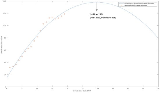
Figure 1.
The amount of carbon emissions and fitting curve for China from 2000 to 2018.
We use population data of China from 2000 to 2019 (Table 3) to make a fitting curve of the population shown in Figure 2.

Table 3.
Data and nature growth rate of population of China.
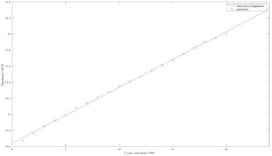
Figure 2.
Population and fitting curve for China from 2000 to 2019.
From Table 3 and Figure 2, we can calculate that the average population growth rate is about . Thus, we choose the natural population growth rate . Meanwhile, according to the common sense of geography, we choose environmental population capacity (Unit: 100 million).
According to the data given in China’s building energy consumption research report, we choose the energy consumption intensity of the building area (Unit: 100 million tons of carbon dioxide/MWh), energy emission intensity .
In the above situation, we assume that China has adopted relevant policies to control carbon emissions. If China only pays attention to economic growth and neglects the control of carbon emissions, the natural growth rate of carbon emissions will be too large to control. Here, we denote the natural growth rate of carbon emissions .
Based on the above analysis, we take two groups of parameters as follows, Group 1:
Group 2:
4.2. The Numerical Simulations
We choose the first group of parameters given in Section 4.1, that is, After calculation, we find that , that is, holds, then exists. We will discuss the stability of the equilibrium in the following part, and . We calculate that , that is, holds and then equilibrium is locally asymptotically stable when . Next, we find that Equation (8) has no positive root. According to Theorem 1, equilibrium is locally asymptotically stable for any . For the initial values (120, 260, 1.4), we show the numerical simulations when and respectively.
When , that is, the increase of carbon emissions has no time delay effect on population growth. From Figure 3, we can find out that after about 13 years, the amount of carbon emissions will reach the peak. That is to say, under the existing policy, China will achieve the goal of emission peak around 2035, and the maximum amount of carbon emissions in the peak state will be about 18 billion tons. After about 80 years, the carbon emissions will gradually decrease and become flat, and China will achieve the goal of carbon neutrality at that time. Corresponding to the emission peak, 10 years after the peak value of carbon emissions, the carbon absorption will reach the peak, then gradually decrease and tend to be flat. And the maximum amount of carbon absorption will be about 31.8 billion tons. This is consistent with the actual situation, so that China can achieve the goal of “double carbon” and make China’s contribution to environmental protection and sustainable development of human society. At the same time, after a very long period of time, the urbanized population can indeed reach a plateau.
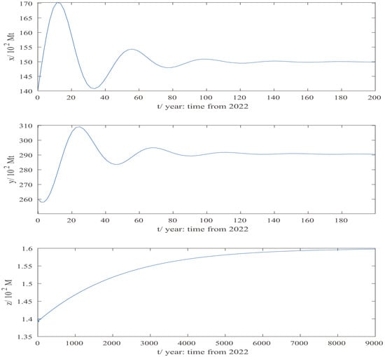
Figure 3.
Equilibrium point of system (3) is locally asymptotically stable when under the first group of parameters.
From the previous analysis, we know that the increase of carbon emissions will have a certain time delay impact on population growth. Because human ecosystems have a certain response time to environmental changes, meanwhile, considering the economic development and urbanization process of the country, this response time is between about three to seven years, so we choose for the numerical simulations. When , that is, the increase of carbon emissions has a five-year time delay effect on population growth. From Figure 4, we can also find out that after about 13 years, the amount of carbon emissions will reach the peak and the maximum amount of carbon emissions will be about 17.8 billion tons. Corresponding to the emission peak, 10 years after the peak value of carbon emissions, the carbon absorption will reach the peak, then gradually decrease and tend to be flat, and the maximum amount of carbon absorption is about 31 billion tons. This is because the increase of carbon emissions has a five-year time delay effect on population growth while the growth of population will accelerate the growth of carbon emissions. So compared with , we can find that the maximum amount of carbon emissions and carbon absorption are a little lower.
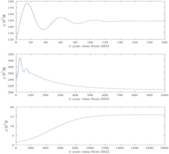
Figure 4.
Equilibrium point of system (3) is locally asymptotically stable when under the first group of parameters.
When we choose the second group of parameters given in Section 4.1, that is,
After calculation, we find that , that is, holds, then exists. So we will discuss the stability of the equilibrium in the following part, and . We calculate that , that is, holds, then, equilibrium is locally asymptotically stable when . Next, we find that Equation (8) has no positive root, according to Theorem 1, equilibrium is locally asymptotically stable for any . For the initial values (120, 260, 1.4), we show the numerical simulations when and respectively.
Comparing Figure 3 with Figure 5 and Figure 4 with Figure 6, we can see that although the amount of carbon emissions will reach the maximum around 2035, the carbon emissions show a cyclical fluctuation and decline in the future. In fact, the peak carbon target cannot be achieved. This is because, after 2035, though the carbon emission is declining, it will reach another peak in certain years. Although these new peaks are smaller than the peak around 2035, they are still at a high level. Therefore, the goal of emission peak cannot be achieved. Corresponding to carbon emissions, carbon absorption also shows a cyclical fluctuation and decline, so we must take measures to control the growth rate of carbon emissions. In this way, the goal of emission peak can be achieved around 2035.
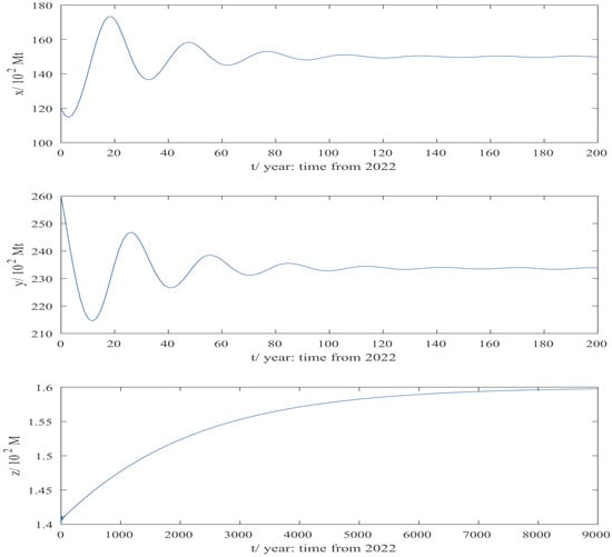
Figure 5.
Equilibrium point of system (3) is locally asymptotically stable when under the second group of parameters.
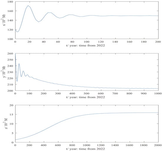
Figure 6.
Equilibrium point of system (3) is locally asymptotically stable when under the second group of parameters.
5. Conclusions
In this paper, considering the relationship among carbon emissions, carbon absorption and urbanization process, we have constructed a delay differential equation model based on China’s urbanization process. Then, we analyzed the existence and stability of the positive equilibrium point of the system, and substituted the actual data for simulations. In the part of numerical simulations, we first selected a reasonable natural growth rate of carbon emissions for simulation. Through simulations, we found that under the current natural growth rate of carbon emissions, China could achieve the goal of emission peak around 2035 and the maximum amount of carbon emissions will be about 17.8 billion tons. Then, by adjusting the natural growth rate of carbon emissions, we found that although the amount of carbon emissions will reach the peak value 18 billion tons around 2035, then it will reach 16 billion tons around 2060 and this value is still at a high level, therefore, we drew a conclusion that the goal of emission peak can not be achieved on schedule if the natural growth rate of carbon emissions is too large. At the same time, we also found that the change of urban population would have a certain impact on the carbon emissions of urban buildings. Also, we take the impact of COVID-19 epidemic into account. Our country spends more funds on epidemic prevention and control. As a result, less money will be spent on urbanization. Meanwhile, the impact of the epidemic can reduce the amount of labor devoted to urbanization. The outbreak of COVID-19 epidemic will cause factories to stop working and production in a short term, then it will cause a slowdown in urbanization. However, in the long turn, after the COVID-19 epidemic, urban public health awareness will be improved, the level of urban environmental protection will be substantially improved. Combining all analysis above, the actual urbanization process will be a little slower than the theoretical urbanization process in our model, but the quality of urbanization will be improved. In fact, this is because mathematical modeling is an idealized process. In the process of modeling, we assume that the parameters are constant, however, in the real situation, the parameters are changing over time.
Therefore, in order to successfully realize the goal of emission peak and carbon neutrality, we suggest that China should take a series of measures to reduce the growth rate of carbon emissions. Firstly, China should adjust energy structure. The adjustment of energy structure is an important way to realize the goal of emission peak and carbon neutrality. China should vigorously promote the use of clean energy and accelerate the replacement of fossil energy. Secondly, China should improve production technology, promote low-carbon, environmentally friendly, clean and sustainable industrial production and processing programs vigorously. Thirdly, we should also pay attention to controlling the growth of carbon emissions in the process of promoting industrial restructuring and upgrading, and we should always put environmental protection on an equal footing with economic and social development. Meanwhile, we should also take measures to increase the natural growth rate of carbon absorption. For example, we can promote afforestation and reforestation to increase the area of forests and urban green areas, then the amount of carbon absorption can be increased. At the same time, in the process of urbanization, we should pay attention to controlling the growth of urban carbon emissions, and focus on implementing measures such as building energy-saving buildings, controlling the rate of urbanization and increasing the area of urban green space which can be taken to reduce the excessive urbanization and accelerate the growth of carbon emissions. At the same time, China should take certain demographic measures, such as “universal two-child policy”, to make the population growth compatible with the economic and social development and urbanization process. In the future, China should vigorously promote new energy and alternative energy of fossil energy, which can also reduce carbon emissions, thus contributing to the realization of the goal of emission peak and carbon neutrality.
Author Contributions
Writing—original draft preparation: H.S. and L.H.; funding acquisition: H.S., L.H. and Y.D.; methodology and supervision: Y.D. All authors have read and agreed to the published version of the manuscript.
Funding
This study was funded by Fundamental Research Funds for the Central Universities of China (Grant No. 2572022DJ06) and College Students Innovations Special Project funded by Northeast Forestry University of China (No. 202210225155).
Institutional Review Board Statement
Not applicable.
Informed Consent Statement
Not applicable.
Data Availability Statement
The authors confirm that the data supporting the findings of this study are available within the article.
Conflicts of Interest
All authors declare no conflict of interest in this paper.
References
- Friedlingstein, P.; Jones, M.W.; O’Sullivan, M.; Andrew, R.M.; Bakker, D.C.; Hauck, J.; Le Quéré, C.; Peters, G.P.; Peters, W.; Pongratz, J.; et al. Global carbon budget 2021. Earth Syst. Sci. Data 2022, 14, 1917–2005. [Google Scholar] [CrossRef]
- Rogelj, J.; Popp, A.; Calvin, K.V.; Luderer, G.; Emmerling, J.; Gernaat, D.; Fujimori, S.; Strefler, J.; Hasegawa, T.; Marangoni, G.; et al. Scenarios towards limiting global mean temperature increase below 1.5 °C. Nat. Clim. Chang. 2018, 8, 325–332. [Google Scholar] [CrossRef]
- Fang, J.Y. Ecological Perspective of Carbon Neutrality. Chin. J. Plant Ecol. 2021, 45, 1173–1176. [Google Scholar] [CrossRef]
- Hacker, J.N.; De Saulles, T.P.; Minson, A.J.; Holmes, M.J. Embodied and operational carbon dioxide emissions from housing: A case study on the effects of thermal mass and climate change. Energy Build. 2008, 40, 375–384. [Google Scholar] [CrossRef]
- Wu, Y.; Xu, B. When will China’s carbon emissions peak? Evidence from judgment criteria and emissions reduction paths. Energy Rep. 2022, 8, 8722–8735. [Google Scholar] [CrossRef]
- Chen, S.; Liu, Y.Y.; Lin, J.; Shi, X.D.; Jiang, K.J.; Zhao, G.L. Coordinated reduction of CO2 emissions and environmental impacts with integrated city-level LEAP and LCA method: A case study of Jinan, China. Adv. Clim. Chang. Res. 2021, 12, 848–857. [Google Scholar] [CrossRef]
- Zhu, C.; Chang, Y.; Li, X.; Shan, M. Factors influencing embodied carbon emissions of China’s building sector: An analysis based on extended STIRPAT modeling. Energy Build. 2022, 255, 111607. [Google Scholar] [CrossRef]
- Ye, L.; Yang, D.; Dang, Y.; Wang, J. An enhanced multivariable dynamic time-delay discrete grey forecasting model for predicting China’s carbon emissions. Energy 2022, 249, 123681. [Google Scholar] [CrossRef]
- Huang, Z.; Dong, H.; Jia, S. Equilibrium pricing for carbon emission in response to the target of carbon emission peaking. Energy Econ. 2022, 112, 106160. [Google Scholar] [CrossRef]
- Agarana, M.C.; Bishop, S.A.; Agboola, O.O. Minimizing carbon emissions from transportation projects in Sub-saharan Africa cities using mathematical model: A Focus on Lagos, Nigeria. Procedia Manuf. 2017, 7, 596–601. [Google Scholar] [CrossRef]
- Hadd, S.; Lahbiri, F.Z. Stochastic Delay-Differential Equations As Bacterial Population Model with boundary feedback. IFAC-PapersOnLine 2022, 55, 202–207. [Google Scholar] [CrossRef]
- Wilson, L.R.M.; Cryer, N.C.; Haughey, E. Simulation of the effect of rainfall on farm-level cocoa yield using a delayed differential equation model. Sci. Hortic. 2019, 253, 371–375. [Google Scholar] [CrossRef]
- Liu, H.; Zhang, J.F. Dynamics of two time delays differential equation model to HIV latent infection. Phys. Stat. Mech. Its Appl. 2019, 514, 384–395. [Google Scholar] [CrossRef]
- Feng, Z.C.; Chicone, C.A. Delay differential equation model for surface acoustic wave sensors. Sens. Actuators Phys. 2003, 104, 171–178. [Google Scholar] [CrossRef]
- Ding, Y.; Zheng, L.; Guo, J. Stability analysis of nonlinear glue flow system with delay. Math. Methods Appl. Sci. 2022, 45, 6861–6877. [Google Scholar] [CrossRef]
Publisher’s Note: MDPI stays neutral with regard to jurisdictional claims in published maps and institutional affiliations. |
© 2022 by the authors. Licensee MDPI, Basel, Switzerland. This article is an open access article distributed under the terms and conditions of the Creative Commons Attribution (CC BY) license (https://creativecommons.org/licenses/by/4.0/).