Abstract
This study developed a method for designing parallel two-degree-of-freedom proportional-integral-derivative controllers for unstable time-delay processes with unknown dynamic equations. First, a performance index accounting for both transient response performance and disturbance rejection was developed. To obtain useful data even if the output of the system exceeds the allowable range, an effective penalty function was included in the performance index. The N–M simplex method was used to iteratively determine the optimal controller parameters. The proposed approach has the following advantages: (1) it can be used regardless of the stability of the open-loop system; (2) the mathematical model and parameters of the process need not be known in advance; (3) it can be used for processes that include measurement noise; (4) it has good transient response performance and is also robust against external disturbances; and (5) it enables more efficient controller design and reduces costs.
1. Introduction
Time delay is a common real-world phenomenon [1,2,3,4,5] because matter and energy exist in a distributed state. A time delay occurs when matter or energy is transported within a medium. Transmission systems, chemical processes, metallurgical processes, hydraulic and pneumatic systems, power systems, biological systems, the environment, and ecosystems are examples of time-delay systems. The existence of time delay complicates the analysis and control of systems. In particular, designing a controller for a time-delay system whose dynamic equation is unknown is challenging.
In most time-delay processes, proportional-integral-derivative (PID) control is used as the feedback controller due to its simple structure and implementation. The design and adjustment of the PID controller are conceptually intuitive. However, designs required to meet multiple objectives at the same time (for example, both good transient response characteristics and disturbance rejection) may be difficult to achieve in practice [6,7,8,9,10].
Many studies have proposed various methods for adjusting PID parameters or parallel two-degree-of-freedom (2-DOF) PID parameters for unstable time-delay systems. For example, Nasution et al. [11] synthesized an optimal H2 PID controller from an internal model control design for unstable processes with a single right-half-plane pole and a time delay. Hast and Hägglund [12] proposed a method for finding the set-point weights of a PID controller by using convex optimization techniques. Begum et al. [13] developed analytical tuning rules for PID controllers for unstable first order plus dead time processes. Chakraborty et al. [14] proposed an integral–proportional derivative (I-PD) control strategy for integrator plus time delay processes. The proposed scheme comprised an inner proportional derivative (PD) loop and an outer integral loop for controlling a servo and for regulatory actions. Verma and Padhy [15] studied the effects of exponential weights on square-of-error functions for PID control systems. They demonstrated that the performance of any process can be tailored by applying exponential weights in the objective function. Onat [16] presented a graphical method for tuning the proportional integral (PI)-PD controller parameters for unstable time-delay systems. The proposed method used a new concept, namely the centroid of the convex stability region. The method only requires the coordinates of a few special points related to the curve determining the stable controller parameter area. Zhang et al. [17] proposed an optimized robust control algorithm based on the mirror mapping method for a class of industrial unstable processes with time delays. Raja and Ali [18] proposed tuning rules for the PI-PD control structure for a class of unstable time-delay processes. The proposed method required the tuning of only four controller parameters.
However, most of the proposed methods in these studies have failed to provide rules for tuning the controller parameters for unstable time-delay processes with unknown mathematical models. Therefore, a trial-and-error method for designing an actual controller is often adopted if information on the approximate or nominal dynamic equation of the process is lacking.
Moreover, during the adjustment of the controller parameters, the process output may exceed the allowable range of variation. If this occurs, the experiment must be immediately terminated, and relevant safety or protective measures must be initiated to prevent injury to the operator or damage to the equipment. If a running experiment is terminated, not only are raw materials and consumables wasted but the obtained data are incomplete and must also be discarded. Therefore, designing a high-performance controller for unstable real-world processes is a not only time consuming but also a potentially expensive task.
To overcome these difficulties in designing real controllers, this study formulated an optimal controller design method for an unstable time-delay process with measurement noise and external disturbance. First, a novel performance index (objective function) was established based on the response requirements of the controlled process. The performance index includes only an explicit function of time and output error; thus, no prior knowledge of the mathematical model of the process is required to calculate the index value. Moreover, a penalty function was included to ensure that the performance index is applicable even if the output of the process is outside the allowable range. In mathematical optimization, penalty functions can be used to solve constrained optimization problems. By introducing a weighted penalty for violating constraints, the constraint problem can be transformed into a nonconstraint problem.
The Nelder–Mead (N–M) simplex method was used to search for the minimum value of the performance index and obtain optimal controller parameters. The N–M simplex method is an algorithm modified by Nelder and Mead [19] on the basis of the simplex method originally proposed by Spendley, Hext, and Himsworth [20]. Because the N–M simplex method is easy to implement and does not require derivatives of the objective function, it is suitable for solving optimization problems if derivatives of the objective function are not available or contain noise [21,22,23,24,25].
To verify the feasibility and effects of the proposed method, several unstable time-delay processes with unknown transfer functions were investigated as examples. In each simulation, the system output contained measurement noise and could only be operated within a limited range. In addition, an external disturbance was added during the second half of each simulation to assess the robustness of the system. The simulation results reveal that even if the initial controller parameters cannot stabilize the process when the algorithm reaches the iterative termination condition, the obtained controller parameters can not only stabilize the process but also have good transient response performance and robustness against external disturbances.
The remaining parts of the article are organized as follows. The mathematical models of the open-loop system and the three 2-DOF PID controllers considered in this paper are described in Section 2. Section 3 discusses the performance index with the penalty function proposed in this paper and discusses the N–M simplex method for identifying the optimal controller parameters. A comparison and analysis of the simulation results is presented in Section 4. Finally, concluding remarks are given in Section 5.
2. System Description
The open-loop system considered in this paper can be represented by the following transfer function:
where denotes the Laplace operator. In addition, the transfer function G and the time delay are unknown. At least one pole of is located in the right half of the complex plane, and can be stabilized by using the parallel 2-DOF PID controller as presented in Figure 1, where is the reference input, is the output, is the error, and is the control input.
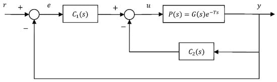
Figure 1.
Block diagram of the system that is controlled by a parallel 2-DOF PID controller.
Here, , , and denote the coefficients (gains) for the proportional, integral, and derivative terms of respectively. The definition of the coefficients in is similar to that for , but the integral term is unnecessary in . We discuss and compare the following three commonly used parallel 2-DOF PID controllers:
- PID controller
Let , , , and . Then, the parallel 2-DOF PID controller degenerates into the following single-DOF PID controller:
- I-PD controller
Define , , , and . The following I-PD controller is then obtained:
- PI-PD controller
Set , , , , and The following PI-PD controller is obtained:
In practical applications, the control system in Figure 1 may be subject to external disturbances and the output signal is also affected by measurement noise . If a filter is added to the output signal, the system block diagram becomes that in Figure 2, where denotes the filter.
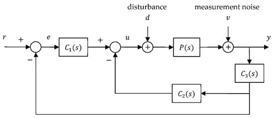
Figure 2.
System block diagram of parallel 2-DOF PID control including the external disturbance , measurement noise , and low-pass filter .
In this paper, was considered as a first-order low-pass filter with the following form:
Here, is the cutoff frequency of the low-pass filter. In practical applications, the approximate transfer function of the open-loop system (Equation (1)) must be obtained using parameter identification techniques. However, if the output signal is disturbed by large-magnitude white noise and the system also uses a low-pass filter, the estimated transfer function would have substantial error; in extreme cases, the result may be meaningless. Thus, many controller design methods based on known open-loop system transfer functions cannot be used. Therefore, the designer can only adjust the controller parameters through trial and error based on experience.
Moreover, the output, , of a real system may indicate temperature, pressure, voltage, current, displacement, or velocity. As with these physical quantities, the actual output value may only be allowed to change within a specific range due to the limitations of the device itself or due to safety considerations. If the output, , exceeds the allowable range of variation, the experiment must be stopped immediately. In this situation, the design of the controller parameters is more difficult and time consuming. To overcome this problem, the N–M simplex method based on a performance index with a penalty function was used to identify the optimal controller parameters. The method is detailed in the next section.
3. Design of Controller Parameters
The N–M simplex method is one of the most famous algorithms for multidimensional unconstrained optimization without derivatives. The N–M simplex method is intended to solve -dimensional unconstrained optimization problems with the following form:
Here, is an vector composed of the controller parameters (controller gains) to be designed, and is a scalar performance index (also called objective function or cost function).
To design an optimal controller, the performance index must first be determined. The performance index is used in the simplex method to search for the optimal points. The performance index must account for factors such as the dynamic characteristics of the system and the desired control target. This function is usually a positive-valued function; smaller output values indicate that the control system is closer to its optimization goal. Some commonly used performance indexes are as follows:
- Integral of absolute error (IAE)
- Integral of squared error (ISE)
- Integral of time-weighted absolute error (ITAE)
- Integral of time-weighted squared error (ITSE)
Here, is the final time of the experiment or simulation.
These performance indexes are typically only a quantitative reference for comparing the performance of different controllers; they do not directly suggest rules or formulas for determining the parameter values of the controllers. For example, most studies regarding the use of PID, I-PD, or PI-PD to control a system with time delay have focused on systems with a transfer function of a specific form by using sufficient numerical calculations or curve fitting methods to obtain an approximately optimal controller parameter formula. To use these methods, the transfer function of the system must first be known. However, estimating the transfer function of an open-loop system that is unstable and has substantial measurement noise is difficult.
To overcome this problem, the N–M simplex method with a performance index and a penalty function was used to search for the optimal controller parameters. Before applying the proposed performance index in this study, the variables and symbols in the index are first defined in Table 1.

Table 1.
Definitions and descriptions of the variables and symbols in the proposed performance index.
The performance index used in this paper is defined as follows:
where
and contain penalty functions. The weight is then determined. First, the most conservative situation is considered in which the error is equal to the maximum value from the beginning and maintained for a time , where is the sampling time. The integral term in Equation (18) is then approximately equal to . To ensure that the penalty function is useful, the following conditions must be satisfied:
That is,
After an appropriate performance index is defined, the N–M simplex method can be applied to systematically search for optimal controller parameters.
The N–M simplex method generates a simplex sequence; each simplex is composed of different vertices , and the corresponding performance index values are respectively. All vertices are assumed to satisfy after sorting according to the performance indexes. Next, and are defined as follows:
In each iteration, the N–M simplex method is used to examine one or more of four different values along the line . These four values are denoted as , , and and must satisfy the following condition:
In practical applications, the typical values are , , and [19,22,23]. The values of , , and yield the reflection point , the expansion point , the outer contraction point , and the inner contraction point , respectively. The values of the performance index at these four points are denoted as , , and , respectively. If none of the four points is superior to the current lowest performance point , the algorithm shrinks the points toward the lowest , thereby producing a new simplex. During the shrinking process, each is replaced by for . Upon the completion of the shrinking process, a new iteration is automatically triggered. This iterative process is continued until the specified termination criteria are satisfied. Table 2 lists the definitions of related names, symbols, and equations in the N–M simplex method.
Table 2.
Definitions of related names, symbols, and equations in the N–M simplex method.
As a simplified example of the N–M simplex method, consider a two-dimensional space (; , ). First, three points that are not on the same straight line are randomly generated or preliminarily selected, and a monomer with , , and is formed (Figure 3). The performance index corresponding with the vertex is represented by . After all the vertices have been sorted according to their performance index size, is satisfied.
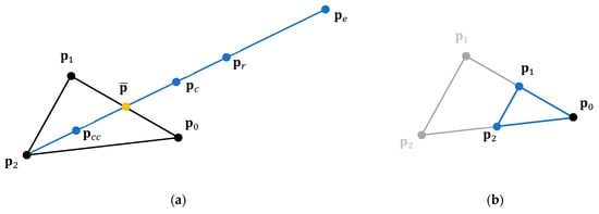
Figure 3.
Diagram of various possible candidate points during each of N–M simplex iteration: (a) linear search; (b) shrink.
In each iteration of the N–M simplex method, an attempt is made to find a superior point through a simplified linear search or shrink method to replace the worst point in the simplex (i.e., ). In the linear search part, some or all of the following four points are considered in each iteration: , , , . This iterative step is repeated to approximate the best solution. The basic steps of the N–M simplex method are summarized in Table 3.
Table 3.
Steps for search for the optimal controller parameters, using the N–M simplex method.
4. Simulation Results
To examine the feasibility and effectiveness of the proposed method, simulations were run for the following cases. Each open-loop system was an unstable process with a time delay. The reference input for all cases was set as , and the allowable range of variation in the output was . Moreover, denotes a constant disturbance to the system. The start time of each simulation was defined as 0. The simulation completion (end) time is denoted as . The disturbance was added to the system at time , and the disturbance continued until . All systems used a first-order low-pass filter, such as that expressed in Equation (11), and the cutoff frequency depended on the system and noise characteristics.
4.1. Case 1
Consider an unstable time-delay process with the following transfer function:
In this case, the sampling time was 0.001, and the preset end time was 10. The target value of the output, was , and the lower limit and upper limits for were and , respectively. The measurement noise, was normally distributed with mean 0 and standard deviation 0.1. The cutoff frequency for the first-order low-pass filter was . An external disturbance was added to the system at time . The termination condition of the N–M simplex algorithm was 50 iterations. The performance index is defined in Equations (17)–(20), where the coefficient of the penalty function was set to according to Inequality (22).
4.1.1. PID Controller
Because the PID controller in this case had three parameters, four sets of controller parameters (gains) were first arbitrarily designated as the four vertices of the initial simplex. Table 4 lists the four sets of initial controller parameters and their corresponding performance indexes. Figure 4 lists the time responses after these four sets of initial parameters were used to control the system.
Table 4.
Initial PID controller parameters of System (26) and their corresponding performance indexes sorted according by the performance indexes.
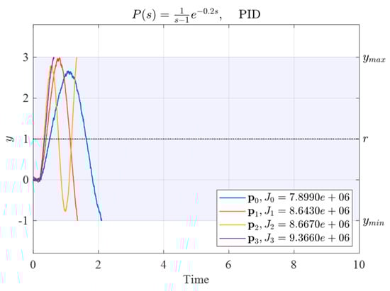
Figure 4.
Time responses after these four sets of initial PID controller parameters were used to control the system.
As indicated by the time responses in Figure 4, all four sets of initial PID controller parameters listed in Table 4 exceeded the allowable range before . Outputs that exceed the allowable safety range earlier have a larger corresponding performance index (i.e., worse controller parameters). Therefore, the proposed penalty function achieved the expected effect.
Subsequently, the aforementioned four sets of parameters were used as the four vertices of the initial simplex. The maximum number of iterations was set as 50. The result for the obtained controller is presented in Figure 5. The parameters of the controller were as follows:
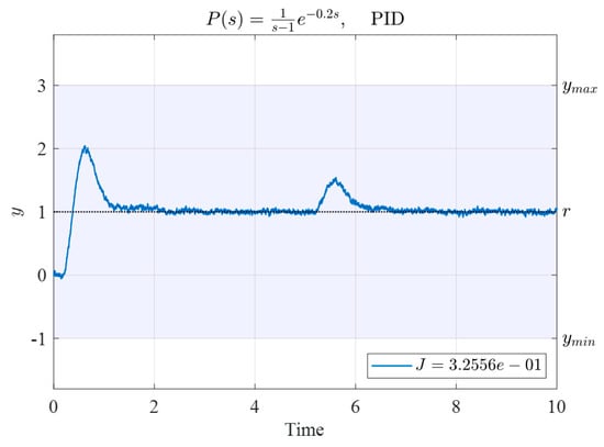
Figure 5.
Time response of System (26) controlled by the PID controller. Gains were found using the N–M simplex method based on the initial vertices given in Table 4.
The corresponding performance index was , far smaller than the performance indexes of the original four sets of controllers (Table 4).
Thus, even if the initial controller parameters result in system instability, our proposed performance index can be used with the N–M algorithm to effectively obtain a set of stable, superior controller parameters.
4.1.2. I-PD Controller
The I-PD controller used in this case also had three parameters; thus, four sets of controller parameters were arbitrarily designated as the four vertices of the initial simplex. The four sets of initial controller parameters and their corresponding performance indexes are listed in Table 5. Figure 6 presents the time responses after these four sets of initial parameters were used to control the system.
Table 5.
Four sets of initial I-PD controller parameters and their corresponding performance indexes for System (26).
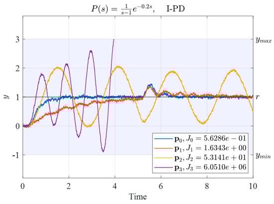
Figure 6.
Time response with these four sets of initial I-PD controller parameters.
As indicated in Figure 6, the parameters , , and could maintain the system output within the allowable range until ; therefore, the penalty function values were 0 and the corresponding index values were small. However, caused the system output to exceed the allowable range before . Therefore, the penalty function achieved the expected effect in that the corresponding index value was much larger than those for , , and .
The aforementioned four sets of parameters were used as the four vertices of the initial simplex. The parameters obtained using the N–M simplex optimal search method are as follows:
The time response using the obtained controller parameters is presented in Figure 7. The corresponding performance index was ; this index was lower than those of the original four sets of controllers.
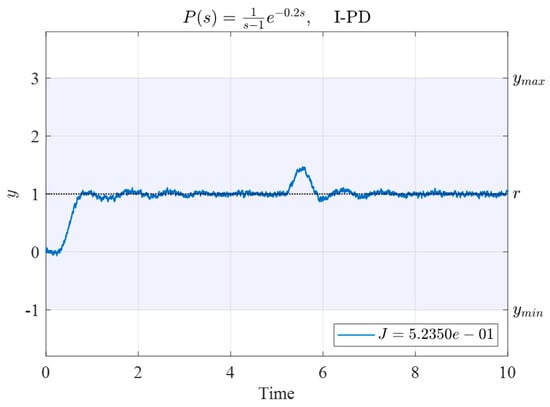
Figure 7.
Time response of System (26) controlled by the I-PD controller with gains obtained using the N–M simplex method based on the initial vertices given in Table 5.
4.1.3. PI-PD Controller
Because the PI-PD controller used in this case had four gains, five sets of controller gains were first arbitrarily designated as the five vertices of the initial simplex. The five sets of gains and their corresponding performance indexes are presented in Table 6. The time responses of the system are presented in Figure 8.
Table 6.
Initial PI-PD controller gains and their corresponding performance indexes for the system (26).
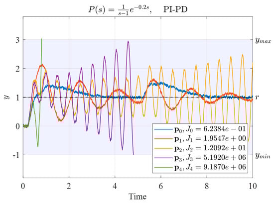
Figure 8.
Time responses after these five sets of initial PI-PD controller gains were used to control System (26).
Among these, the parameters , , and could maintain the system output within the allowable range until ; therefore, all their penalty function values were 0 and the corresponding index values were small. Both and caused the system output to exceed the allowable range before . Therefore, the penalty function achieved the expected effect; the index values were larger than those for the other parameter sets. This result also indicated that parameter sets that caused earlier simulation interruption have larger corresponding index values (indicating worse controller parameters).
Similarly, the aforementioned five sets of controller parameters were applied as the vertices of the initial simplex (Figure 9). The resulting controller parameters obtained by using the N–M simplex optimal search method were as follows:
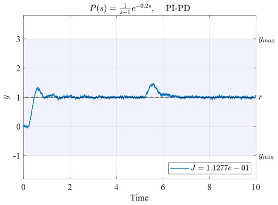
Figure 9.
Time response of System (26) controlled by the PI-PD controller. The controller parameters were obtained using the N–M simplex method with the initial vertices given in Table 6.
The corresponding performance index was ; this value was lower than those of the original five sets of controllers.
4.2. Case 2
We consider a second-order unstable time-delay process with the following transfer function:
In this case, the sampling time was 0.005 and the preset end time, was 50. The target value of the output, was , and and . The measurement noise, was normally distributed with a mean of 0 and standard deviation of 0.1. The cutoff frequency of the first-order low-pass filter was . The external disturbance was injected into the system at . The termination condition of the N–M simplex algorithm was 30 iterations. The performance index was defined as in Equations (17)–(20), and the coefficient of the penalty function was set to according to Inequality (22).
4.2.1. PID Controller
We arbitrarily selected four sets of parameters as the four vertices for the initial simplex for System (30). Table 7 presents four sets of initial controller parameters and their corresponding performance indexes. The time responses obtained using these four sets of controllers are presented in Figure 10.
Table 7.
Four sets of initial PID controller parameters used by System (30) and their corresponding performance indexes.
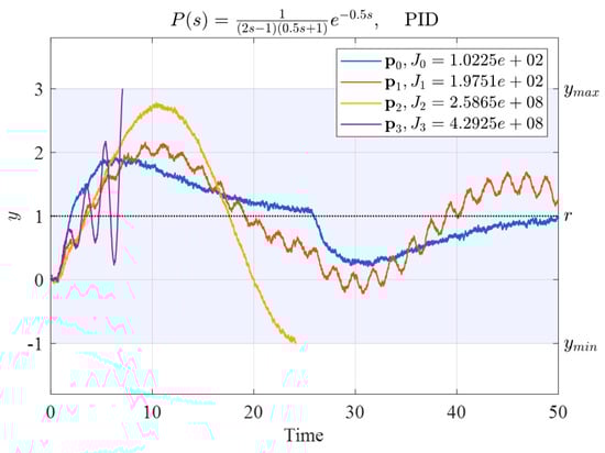
Figure 10.
Output responses of System (30) controlled by the four sets of PID parameters listed in Table 7.
For System (30), the optimal PID controller parameters obtained by the N–M simplex method were as follows:
The output response using these controller parameters is presented in Figure 11, and its corresponding performance index value was .
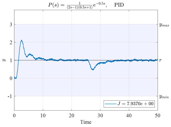
Figure 11.
Time response of System (30) controlled by the PID controller with gains obtained using the N–M simplex method and based on the initial vertices given in Table 7.
4.2.2. I-PD Controller
Similarly, four sets of parameters as the four vertices of the initial simplex were arbitrarily selected to design the I-PD controller for System (30). The four sets of initial controller parameters and their corresponding performance indexes are presented in Table 8. The time responses obtained using these four sets of controllers are presented in Figure 12.
Table 8.
Four sets of initial I-PD controller parameters and their corresponding performance indexes for System (30).
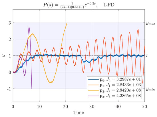
Figure 12.
Time responses of System (30) controlled by the four sets of initial I-PD controller parameters listed in Table 8.
Figure 12 reveals that both and caused range violations before . The corresponding performance indexes were thus large. Although the controller parameters and did not cause range violations, the output corresponding to parameter gradually diverged, and the output corresponding to the parameter was convergent. Therefore, the performance index of was smaller than that of .
The aforementioned four sets of parameters were used as the four vertices of the initial simplex. The parameters obtained using the N–M simplex optimal search method were as follows:
The time response of System (30) with the parameters given in (32) is presented in Figure 13. The corresponding performance index was , which is significantly lower than those of the initial four sets of controllers.

Figure 13.
Time response of System (30) controlled by the I-PD controller with gains obtained by the N–M simplex method and based on the initial vertices given in Table 8.
4.2.3. PI-PD Controller
Table 9 lists five sets of initial parameters and corresponding performance indexes for the PI-PD controller for System (30). The time response of the system is presented in Figure 14.
Table 9.
Initial PI-PD controller gains and their corresponding performance indexes for System (30).
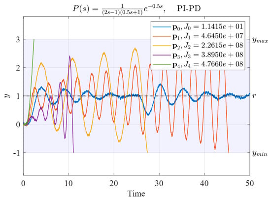
Figure 14.
Time responses using these five sets of initial PI-PD controller gains to control System (30).
The aforementioned five sets of controller parameters were used as the vertices of the initial simplex. The resulting controller gains obtained using the N–M simplex optimal search method were as follows:
The time response of System (30) controlled by the above PI-PD controller is presented in Figure 15. The corresponding performance index was , substantially lower than those of the initial four sets of controllers in Table 9.
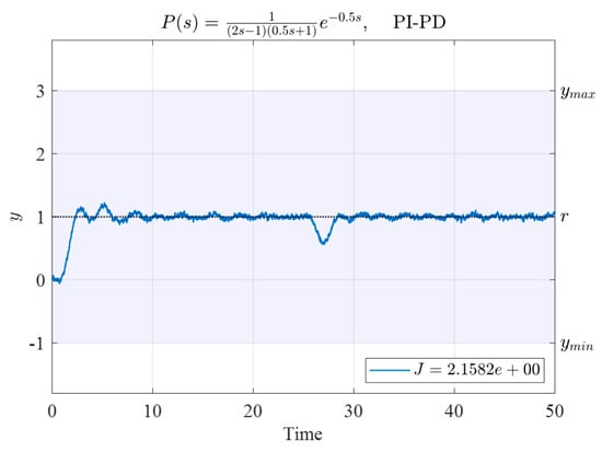
Figure 15.
Time response of System (30) controlled by the PI-PD controller. Controller parameters were obtained with the N–M simplex method using the initial vertices given in Table 9.
4.3. Case 3
Consider another second-order unstable time-delay process with the following transfer function:
In this case, the sampling time was 0.005, and the preset control end time, was 50. The target value of the output, was , and and . The measurement noise, was normally distributed and had a mean of 0 and standard deviation of 0.1. The cutoff frequency of the first-order low-pass filter was . The external disturbance was injected into the system at time . The termination condition of the N–M simplex algorithm was 30 iterations. The performance index is defined as in Equations (17)–(20), and the coefficient of the penalty function was set to according to Inequality (22).
4.3.1. PID Controller
Four sets of initial PID controller gains and their corresponding performance indexes are listed in Table 10. The time responses obtained by using these four sets of controllers are displayed in Figure 16.
Table 10.
Four sets of initial PID controller parameters used by System (34) and their corresponding performance indexes.
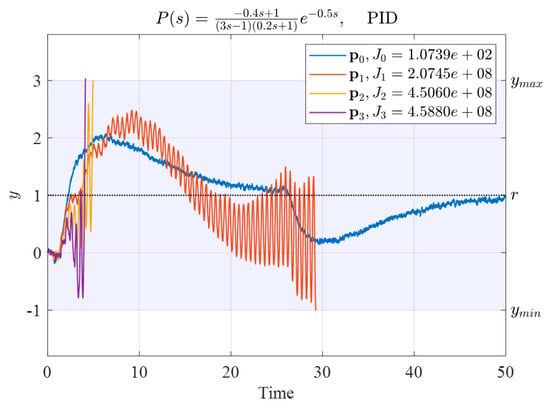
Figure 16.
Output responses of System (34) controlled by the initial PID gains listed in Table 10.
In this case, the optimal PID controller parameters searched by the N–M simplex method were as follows:
The time response of the system using this controller parameter is presented in Figure 17, and its corresponding performance index value was .
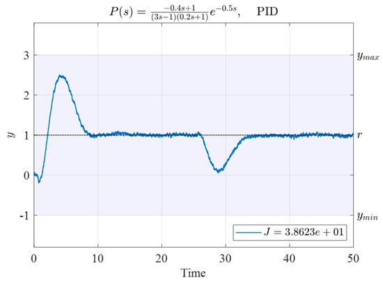
Figure 17.
Time response of System (34) controlled by the PID controller with gains obtained using the N–M simplex method and based on the initial vertices given in Table 10.
4.3.2. I-PD Controller
The four sets of initial controller parameters and their corresponding performance indexes for the I-PD controller for System (34) are listed in Table 11. The time responses obtained by using these controllers are displayed in Figure 18.
Table 11.
Four sets of initial I-PD controller parameters and their corresponding performance indexes for System (34).
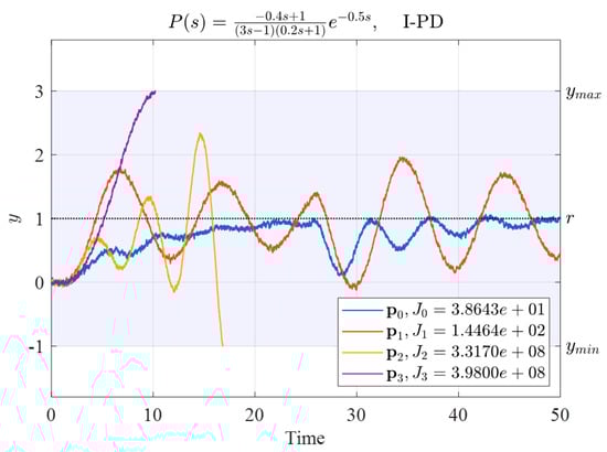
Figure 18.
Time responses of System (34) controlled by the four sets of initial I-PD controller parameters listed in Table 11.
The aforementioned four sets of parameters were then used as the four vertices of the initial simplex. The controller parameters obtained using the N–M simplex optimal search method were as follows:
The time response of the system controlled by the I-PD with gain as in (32) is displayed in Figure 19. The corresponding performance index was , which was lower than those of the initial four sets of controllers.
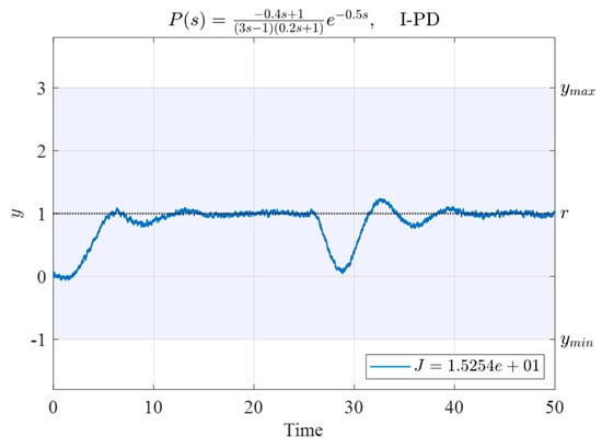
Figure 19.
Time response of System (34) controlled by the I-PD controller with gains obtained using the N–M simplex method based on the initial vertices given in Table 11.
4.3.3. PI-PD Controller
Similarly, five sets of initial controller parameters and their corresponding performance indexes for the PI-PD controller for System (34) are listed in Table 12. The time response of the system is displayed in Figure 20.
Table 12.
Initial PI-PD controller gains and corresponding performance indexes for System (34).
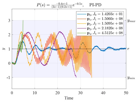
Figure 20.
Time responses using these five sets of initial PI-PD controller gains to control System (34).
The aforementioned five sets of controller parameters were used as the vertices of the initial simplex. The resulting gains obtained using the N–M simplex optimal search method are as follows:
Figure 21 is the time response of System (34) controlled by the above PI-PD controller. The corresponding performance index is ; this is also substantially lower than those of the initial controller parameters presented in Table 12.
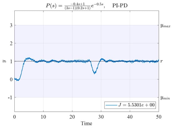
Figure 21.
Time response of System (34) controlled by the PI-PD controller with controller parameters obtained using the N–M simplex method with initial vertices as in Table 12.
4.4. Summary of Cases 1 to 3
The simulation results reveal that, for an unstable time-delay system with an unknown transfer function, the performance index proposed in this paper combined with the N–M simplex algorithm can be effectively used to design stable controller parameters with superior performance. The performance indexes corresponding to the various successful controllers used in Cases 1 to 3 are listed Table 13.
Table 13.
Performance indexes corresponding to the obtained controllers from Cases 1–3.
Table 13 reveals that, with the same performance index, the performance of the PI-PD controller is superior to that of the other two controllers because the PI-PD controller has one more adjustable parameter than the other two controllers do. To identify a controller with better performance, a 2-DOF PID controller with a complete set of five independently adjustable parameters could be used as in Equation (4). The method proposed in this paper could then be used to obtain optimal controller parameters.
5. Conclusions
In this paper, a method for designing parallel 2-DOF PID controllers for unstable time-delay processes with unknown transfer functions was proposed. First, a performance index including both the target value response performance and disturbance rejection was developed. Moreover, to gain value from the incomplete data obtained if the output of the system exceeds the allowable range, an effective penalty function was included in the performance index. The N–M simplex method was then used to iteratively search for optimal controller parameters. The N–M simplex method is advantageous because the algorithm is easy to implement and the system dynamic equations do not need to be known in advance.
To verify the feasibility and effects of the proposed method, several unstable time-delay processes with unknown transfer functions were used as example cases. In these simulations, the output signal of each system contained measurement noise, and the control input was also subject to an external disturbance. Moreover, to increase the similarity to real-world processes, a limit was set on the range of the system output. If the output exceeded the allowable range, the simulation or experiment could be terminated immediately. Although the data obtained from terminated simulations were incomplete, the penalty function enabled the calculation of a meaningful performance index value. Thus, the N–M simplex algorithm could identify the optimal parameters smoothly and recursively. This feature can not only reduce waste in practical applications but also enable the efficient design of controller parameters with superior performance. The simulation results reveal that even if the initial controller parameters result in system instability, the closed-loop system with the final parameters is not only stable but also has good transient response performance.
This paper presents an optimal controller parameter search method for unstable time-delay systems with an unknown transfer function. It has the following advantages: (1) it can be used for unstable processes in an open-loop system; (2) the dynamic equations of the systems can be unknown; (3) it can be used in systems that include measurement noise; (4) it can balance transient response performance and robustness against external disturbances; and (5) its systematic nature makes design more efficient.
Future designers encountering constraints in a controlled system or attempting to find a global optimal controller could modify or add an integral term or penalty function to the performance index in accordance with the concepts proposed in this paper. Design goals could be achieved in combination with global optimization methods.
Author Contributions
Conceptualization, H.-H.T. and C.-C.F.; software, C.-C.F.; validation, H.-H.T. and C.-C.F.; resources, P.-C.T.; writing—original draft preparation, H.-H.T. and C.-C.F.; writing—review and editing, H.-H.T., C.-C.F., J.-R.H., C.-K.L. and P.-C.T.; project administration, C.-C.F. and P.-C.T.; funding acquisition, P.-C.T. and H.-H.T. All authors have read and agreed to the published version of the manuscript.
Funding
This work was supported by the Ministry of Science and Technology, Taiwan, ROC, under Grant MOST 110-2218-E-008-008-.
Institutional Review Board Statement
Not applicable.
Informed Consent Statement
Not applicable.
Data Availability Statement
Not applicable.
Conflicts of Interest
The authors declare no conflict of interest.
References
- Fridman, E. Introduction to Time-Delay Systems: Analysis and Control; Springer: Berlin/Heidelberg, Germany, 2014. [Google Scholar]
- Birs, I.; Muresan, C.; Nascu, I.; Ionescu, C. A Survey of Recent Advances in Fractional Order Control for Time Delay Systems. IEEE Access 2019, 7, 30951–30965. [Google Scholar] [CrossRef]
- Liu, K.; Selivanov, A.; Fridman, E. Survey on Time-Delay Approach to Networked Control. Annu. Rev. Control 2019, 48, 57–79. [Google Scholar] [CrossRef]
- Sun, J.; Su, G.; Chen, X. Data-Driven Controller Synthesis for Parameters Unknown Linear-Delay Systems with Input Constraint. In Proceedings of the 33rd Chinese Control and Decision Conference (CCDC), Kunming, China, 22–24 May 2021; IEEE: Piscataway, NJ, USA; pp. 5915–5920. [Google Scholar] [CrossRef]
- Briones, O.A.; Rojas, A.J.; Sbarbaro, D. Generalized Predictive PI Controller: Analysis and Design for Time Delay Systems. In Proceedings of the 2021 American Control Conference (ACC), New Orleans, LA, USA, 25–28 May 2021; IEEE: Piscataway, NJ, USA; pp. 2509–2514. [Google Scholar] [CrossRef]
- Ravikishore, C.; Praveen Kumar, D.T.V.; Padma Sree, R. Enhanced Performance of PID Controllers for Unstable Time Delay Systems Using Direct Synthesis Method. Indian Chem. Eng. 2021, 63, 293–309. [Google Scholar] [CrossRef]
- Balaguer, V.; González, A.; García, P.; Blanes, F. Enhanced 2-DOF PID Controller Tuning Based on an Uncertainty and Disturbance Estimator with Experimental Validation. IEEE Access 2021, 9, 99092–99102. [Google Scholar] [CrossRef]
- Feng, Z.Y.; Guo, H.; She, J.; Xu, L. Weighted Sensitivity Design of Multivariable PID Controllers via a New Iterative LMI Approach. J. Process. Control 2022, 110, 24–34. [Google Scholar] [CrossRef]
- Tognetti, E.S.; de Oliveira, G.A. Robust State Feedback-Based Design of PID Controllers for High-Order Systems with Time-Delay and Parametric Uncertainties. J. Control Autom. Electr. Syst. 2022, 33, 1–11. [Google Scholar] [CrossRef]
- Dubey, V.; Goud, H.; Sharma, P.C. Role of PID Control Techniques in Process Control System: A Review. In Data Engineering for Smart Systems; Springer: Berlin/Heidelberg, Germany, 2022; pp. 659–670. [Google Scholar]
- Nasution, A.A.; Jeng, J.C.; Huang, H.P. Optimal H2 IMC-PID Controller with Set-Point Weighting for Time-Delayed Unstable Processes. Ind. Eng. Chem. Res. 2011, 50, 4567–4578. [Google Scholar] [CrossRef]
- Hast, M.; Hägglund, T. Optimal Proportional–Integral–Derivative Set-Point Weighting and Tuning Rules for Proportional Set-Point Weights. IET Control Theory Appl. 2015, 9, 2266–2272. [Google Scholar] [CrossRef]
- Begum, K.G.; Rao, A.S.; Radhakrishnan, T.K. Maximum Sensitivity Based Analytical Tuning Rules for PID Controllers for Unstable Dead Time Processes. Chem. Eng. Res. Des. 2016, 109, 593–606. [Google Scholar] [CrossRef]
- Chakraborty, S.; Ghosh, S.; Naskar, A.K. I–PD Controller for Integrating plus Time-Delay Processes. IET Control Theory Appl. 2017, 11, 3137–3145. [Google Scholar] [CrossRef]
- Verma, B.; Padhy, P.K. Optimal PID Controller Design with Adjustable Maximum Sensitivity. IET Control Theory Appl. 2018, 12, 1156–1165. [Google Scholar] [CrossRef]
- Onat, C. A New Design Method for PI–PD Control of Unstable Processes with Dead Time. ISA Trans. 2019, 84, 69–81. [Google Scholar] [CrossRef] [PubMed]
- Zhang, G.; Tian, B.; Zhang, W.; Zhang, X. Optimized Robust Control for Industrial Unstable Process via the Mirror-Mapping Method. ISA Trans. 2019, 86, 9–17. [Google Scholar] [CrossRef] [PubMed]
- Raja, G.L.; Ali, A. New PI-PD Controller Design Strategy for Industrial Unstable and Integrating Processes with Dead Time and Inverse Response. J. Control Autom. Electr. Syst. 2021, 32, 266–280. [Google Scholar] [CrossRef]
- Nelder, J.A.; Mead, R. A Simplex Method for Function Minimization. Comput. J. 1965, 7, 308–313. [Google Scholar] [CrossRef]
- Spendly, W.; Hext, G.R.; Himsworth, F.R. Sequential Application of Simplex Designs in Optimization and Evolutionary Operation. Technometrics 1962, 4, 441–461. [Google Scholar] [CrossRef]
- Lagarias, J.C.; Reeds, J.A.; Wright, M.H.; Wright, P.E. Convergence Properties of the Nelder-Mead Simplex Method in Low Dimensions. SIAM J. Optim. 1998, 9, 112–147. [Google Scholar] [CrossRef] [Green Version]
- McKinnon, K.I.M. Convergence of the Nelder-Mead Simplex Method to a Nonstationary Point. SIAM J. Optim. 1998, 9, 148–158. [Google Scholar] [CrossRef]
- Price, C.J.; Coope, I.D.; Byatt, D. A Convergent Variant of the Nelder-Mead Algorithm. J. Optim. Theory Appl. 2002, 113, 5–19. [Google Scholar] [CrossRef] [Green Version]
- Fuh, C.C.; Tsai, H.H. Applying the Simplex Method to Design the Optimal Parameters of a Sliding Mode Controller for a System with Input Saturation and Unknown Disturbance Bound. IEEE Access 2021, 9, 149100–149109. [Google Scholar] [CrossRef]
- Izci, D.; Hekimoğlu, B.; Ekinci, S. A New Artificial Ecosystem-Based Optimization Integrated with Nelder-Mead Method for PID Controller Design of Buck Converter. Alex. Eng. J. 2022, 61, 2030–2044. [Google Scholar] [CrossRef]
Publisher’s Note: MDPI stays neutral with regard to jurisdictional claims in published maps and institutional affiliations. |
© 2022 by the authors. Licensee MDPI, Basel, Switzerland. This article is an open access article distributed under the terms and conditions of the Creative Commons Attribution (CC BY) license (https://creativecommons.org/licenses/by/4.0/).