Identification of Linear Time-Invariant Systems with Dynamic Mode Decomposition

Abstract

Dynamic mode decomposition (DMD) is a popular data-driven framework to extract linear dynamics from complex high-dimensional systems. In this work, we study the system identification properties of DMD. We first show that DMD is invariant under linear transformations in the image of the data matrix. If, in addition, the data are constructed from a linear time-invariant system, then we prove that DMD can recover the original dynamics under mild conditions. If the linear dynamics are discretized with the Runge–Kutta method, then we further classify the error of the DMD approximation and detail that for one-stage Runge–Kutta methods; even the continuous dynamics can be recovered with DMD. A numerical example illustrates the theoretical findings.

1. Introduction

Dynamical systems play a fundamental role in many modern modeling approaches of physical and chemical phenomena. The need for high fidelity models often results in large-scale dynamical systems, which are computationally demanding to solve, analyze, and optimize. Thus the last three decades have seen significant efforts to replace the so-called full-order model, which is considered the truth model, with a computationally cheaper surrogate model. In the context of model order reduction, we refer the interested reader to the monographs [1,2,3,4,5]. Often, the surrogate model is constructed by projecting the dynamical system onto a low-dimensional manifold, thus requiring a state-space description of the differential equation.

If a mathematical model is not available or not suited for modification, data-driven methods, such as the Loewner framework [6,7], vector fitting [8,9,10], operator inference [11], or dynamic mode decomposition (DMD) [12] may be used to create a low-dimensional realization directly from the measurement or simulation data of the system. Suppose the dynamical system that creates the data is linear. In that case, the Loewner framework and vector fitting are—under some technical assumptions—able to recover the original dynamical system and hence serve as system identification tools. Despite the popularity of DMD, a similar analysis seems to be missing, and this paper aims to close this gap.

Since DMD creates a discrete, linear time-invariant dynamical system from data, we are interested in answering the following questions:

• What is the impact of transformations of the data on the resulting DMD approximation?
• Assume that the data used to generate the DMD approximation are obtained from a linear differential equation. Can we estimate the error between the continuous dynamics and the DMD approximation?
• Are there situations in which we are even able to recover the original dynamical system from its DMD approximation?

It is essential to know how the data for the construction of the DMD model are generated to answer these questions. Assuming exact measurements of the solution may be valid from a theoretical perspective only. Instead, we take the view of a numerical analyst and assume that the data are obtained via time integration of the dynamics with a general Runge–Kutta method (RKM) with known order of convergence. We emphasize that for linear time-invariant systems, a RKM may not be the method of choice; see, for instance, [13]. Nevertheless, RKMs are a common numerical technique to solve general differential equations, which is our main reason to consider RKMs in the following.

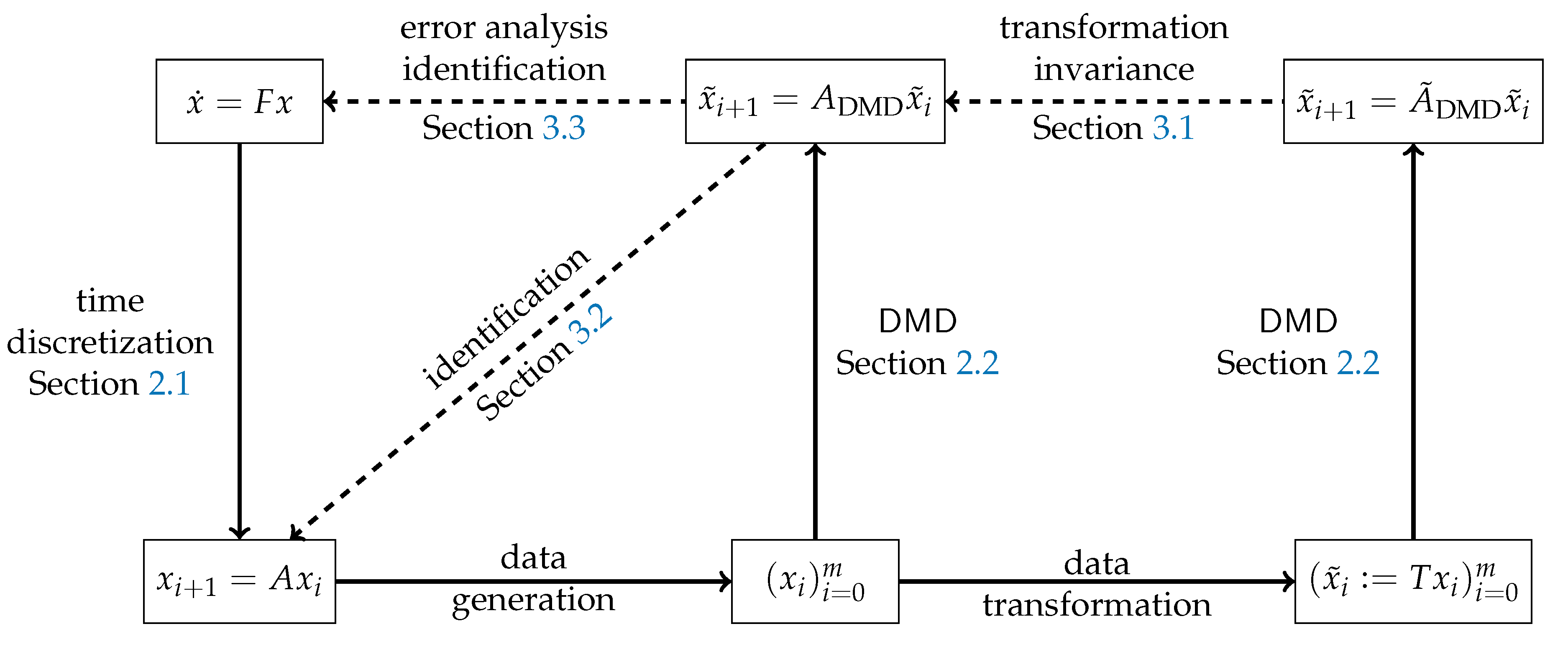
We can summarize the questions graphically as in Figure 1. Thus, the dashed lines represent the questions that we aim to answer in this paper.

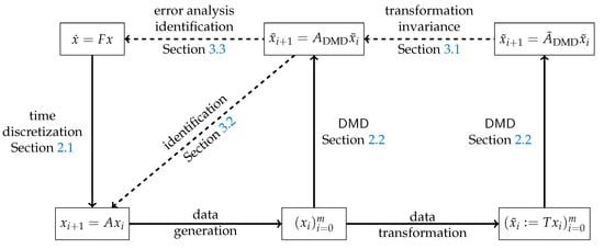
Figure 1. Problem setup.

Our main results are the following:

• We show in Theorem 1 that DMD is invariant in the image of the data under linear transformations of the data.
• Theorem 2 details that DMD is able to identify discrete-time dynamics, i.e., for every initial value in the image of the data, the DMD approximation exactly recovers the discrete-time dynamics.
• In Theorem 3, we show that if the DMD approximation is constructed from data that are obtained via a RKM, then the approximation error of DMD with respect to the ordinary differential equation is in the order of the error of the RKM. If a one-stage RKM is used and the data are sufficiently rich, then the continuous-time dynamics, i.e., the matrix F in Figure 1, can be recovered cf. Lemma 1.

To render the manuscript self-contained, we recall important definitions and results for RKM and DMD in the upcoming Section 2.1 and Section 2.2, respectively, before we present our analysis in Section 3. We conclude with a numerical example to confirm the theoretical findings.

Notation

As is standard, $\mathbb{N}$, $\mathbb{R}$, and $\mathbb{R}\left[t\right]$ denote the positive integers, the real numbers, and the polynomials with real coefficients, respectively. For any $n,m\in \mathbb{N}$, we denote with ${\mathbb{R}}^{n\times m}$ the set of $n\times m$ matrices with real entries. The set of nonsingular matrices of size $n\times n$ is denoted with ${\mathrm{GL}}_n\left(\mathbb{R}\right)$. Let $A=\left[a_{ij}\right]\in {\mathbb{R}}^{n\times m}$, $B\in {\mathbb{R}}^{p\times q}$, and $x_i\in {\mathbb{R}}^n$ ($i=1,\dots ,k$). The transpose and the Moore–Penrose pseudoinverse of A are denoted with $A^T$ and $A^{†}$, respectively. The Kronecker product ⊗ is defined as

$$A\otimes B=\left[\begin{array}{ccc}{a}_{11}B& \cdots & a_{1m}B\\ ⋮& & ⋮\\ a_{n1}B& \cdots & a_{nm}B\end{array}\right]\in {\mathbb{R}}^{np\times mq}.$$

We use $span\{x_1,\dots ,x_k\}$ to denote the linear span of the vectors $x_1,\dots ,x_k$ and also casually write $span\left\{X\right\}=span\{x_1,\dots ,x_k\}$ for the column space of the matrix X with $\{x_1,\dots ,x_k\}$ as its columns. For $A\in {\mathbb{R}}^{n\times n}$ and a vector $x_0\in {\mathbb{R}}^n$, we denote the reachable space as $\mathcal{C}(x_0,A)=span\{x_0,A{x}_0,\cdots ,A^{n-1}{x}_0\}$. The Stiefel manifold of $n\times r$ dimensional matrices with real entries is denoted by

$$\mathrm{St}(n,r)=\left\{U\in {\mathbb{R}}^{n\times r}\mid U^{T}U=I_r\right\},$$

(1)

where $I_r$ denotes the $r\times r$ identity matrix. For a continuously differentiable function $x:\mathbb{I}\to {\mathbb{R}}^n$ from the interval $\mathbb{I}\subseteq \mathbb{R}$ to the vector space ${\mathbb{R}}^n$, we use the notation $\dot{x}:=\frac{\mathrm{d}}{\mathrm{d}t}x$ to denote the derivative with respect to the independent variable t, which we refer to as the time.

2. Preliminaries

As outlined in the introduction, DMD creates a finite-dimensional linear model to approximate the original dynamics. Thus, in view of possibly exact system identification, we need to assume that the data that are fed to the DMD algorithm are obtained from a linear ODE, which in the sequel is denoted by

$$\dot{x}\left(t\right)=Fx\left(t\right)$$

(2a)

with given matrix $F\in {\mathbb{R}}^{n\times n}$. To fix a solution of (2a), we prescribe the initial condition

$$x\left(0\right)=x_0\in {\mathbb{R}}^n,$$

(2b)

and denote the solution of the initial value problem (IVP) as $x(t;x_0):=exp\left(Ft\right)x_0$. For the analysis of DMD, we assume that the matrix F is not available. Instead, the question is to what extent DMD is able to recover the matrix F solely from measurements of the state variable x.

Remark 1.

While a DMD approximation, despite its linearity, may well reproduce trajectories of nonlinear systems (see, for example, [14]), the question of DMD being able to recover the full dynamics has to focus on linear systems. Here, the key observation is that a DMD approximation is a finite-dimensional linear map. In contrast, the encoding of nonlinear systems via a linear operator necessarily needs an infinite-dimensional mapping.

2.1. Runge–Kutta Methods

To solve the IVP (2) numerically, we employ a RKM, which is a common one-step method to approximate ordinary and differential-algebraic equations [15,16]. More precisely, given a step size $h>0$, the solution of the IVP (2) is approximated via the sequence $x_i\approx x(t_0+ih)$ given by

$$x_{i+1}=x_i+h\sum _{j=1}^s{\beta }_j{k}_j,$$

(3a)

with the so-called internal stages $k_j\in {\mathbb{R}}^n$ (implicitly) defined via

$$k_j=F{x}_i+h\sum _{\ell =1}^s{\alpha }_{j,\ell }F{k}_{\ell }\mathrm{for}j=1,\dots ,s,$$

(3b)

where $s\in \mathbb{N}$ denotes the number of stages in the RKM. Using the matrix notation $\mathcal{A}=\left[{\alpha }_{j,\ell }\right]\in {\mathbb{R}}^{s\times s}$ and $\beta =\left[{\beta }_j\right]\in {\mathbb{R}}^s$, the s-stage RKM defined via (3) is conveniently summarized with the pair $(\mathcal{A},\beta )$. Note that we restrict our presentation to linear time-invariant dynamics, and hence, do not require the full Butcher tableau.

Since the ODE (2a) is linear, we can rewrite the internal stages as

$$\left[\begin{array}{cccc}{I}_n-h{\alpha }_{1,1}F& -h{\alpha }_{1,2}F& \dots & -h{\alpha }_{1,s}F\\ -h{\alpha }_{2,1}F& I_n-h{\alpha }_{2,2}F& \dots & -h{\alpha }_{2,s}F\\ ⋮& \ddots & \ddots & ⋮\\ -h{\alpha }_{s,1}F& \cdots & -h{\alpha }_{s,s-1}F& I_n-h{\alpha }_{s,s}F\end{array}\right]\left[\begin{array}{c}{k}_1\\ k_2\\ ⋮\\ k_s\end{array}\right]=\left[\begin{array}{c}F{x}_i\\ F{x}_i\\ ⋮\\ F{x}_i\end{array}\right]$$

(4)

Setting $k:={\left[\begin{array}{ccc}{k}_1^T& \dots & k_s^T\end{array}\right]}^T\in {\mathbb{R}}^{sn}$ and $e:={\left[\begin{array}{cc}1& \dots 1\end{array}\right]}^T\in {\mathbb{R}}^s$, the linear system in (4) can be written as

$$(I_s\otimes I_n-h\mathcal{A}\otimes F)k=(e\otimes F)x_i,$$

(5)

where ⊗ denotes the Kronecker product. If h is small enough, the matrix $(I_s\otimes I_n-h\mathcal{A}\otimes F)$ is invertible, and thus, we obtain the discrete linear system

$$\begin{array}{cc}\hfill x_{i+1}& =x_i+h\sum _{j=1}^s{\beta }_j{k}_j=x_i+h({\beta }^T\otimes I_n)k\hfill \\ \hfill & =x_i+h({\beta }^T\otimes I_n){\left(I_s\otimes I_n-h\mathcal{A}\otimes F\right)}^{-1}(e\otimes F)x_i=A_h{x}_i,\hfill \end{array}$$

with (using the identity $I_s\otimes I_n=I_{sn}$)

$$A_h:=I_n+h({\beta }^T\otimes I_n){\left(I_{sn}-h\mathcal{A}\otimes F\right)}^{-1}(e\otimes F).$$

(6)

Example 1.

The explicit (or forward) Euler method is given as $(\mathcal{A},\beta )=(0,1)$ and according to (6) we obtain the well-known formula $A_h=I_n+hF$. For the implicit (or backward) Euler method $(\mathcal{A},\beta )=(1,1)$ the discrete system matrix is given by

$$A_h=I_n+h{(I_n-hF)}^{-1}F={(I_n-hF)}^{-1}(I_n-hF+hF)={(I_n-hF)}^{-1}.$$

To guarantee that the representation (6) is valid, we make the following assumption throughout the manuscript.

Assumption A1.

For any s-stage RKM $(\mathcal{A},\beta )$ and any dynamical system matrix $F\in {\mathbb{R}}^{n\times n}$, we assume that the step size h is chosen such that the matrix $I_{sn}-h\mathcal{A}\otimes F$ is nonsingular.

Remark 2.

Using Assumption 1, the matrix $I_{sn}-h\mathcal{A}\otimes F$ is nonsingular, and thus, there exists a polynomial $p={\sum }_{k=0}^{sn-1}{p}_k{t}^k\in \mathbb{R}\left[t\right]$ of degree at most $sn-1$ depending on the step size h such that

$$\begin{array}{cc}\hfill {\left(I_{sn}-h\mathcal{A}\otimes F\right)}^{-1}& =p(I_{sn}-h\mathcal{A}\otimes F)=\sum _{k=0}^{sn-1}{p}_k{\left(I_{sn}-h\mathcal{A}\otimes F\right)}^k\hfill \\ \hfill & =\sum _{k=0}^{sn-1}{p}_k\sum _{\rho =0}^k\left(\genfrac{}{}{0pt}{}{k}{\rho }\right){(-1)}^{\rho }{h}^{\rho }({\mathcal{A}}^{\rho }\otimes F^{\rho }),\hfill \end{array}$$

where the last equality follows from the binomial theorem. Consequently, we have

$$\begin{array}{c}\hfill A_h=I_n+\sum _{k=0}^{sn-1}{p}_k\sum _{\rho =0}^k\left(\genfrac{}{}{0pt}{}{k}{\rho }\right){(-1)}^{\rho }{h}^{\rho +1}\left({\beta }^T{\mathcal{A}}^{\rho }e\right)F^{\rho +1}.\end{array}$$

(7)

Rearranging the terms together with the Cayley–Hamilton theorem implies the existence of a polynomial $\tilde{p}\in \mathbb{R}\left[t\right]$ of degree at most n such that $A_h=\tilde{p}\left(F\right)$. As a direct consequence, we see that any eigenvector of F is an eigenvector of $A_h$ and thus, $A_h$ is diagonalizable if F is diagonalizable.

Having computed the matrix $A_h$, the question that remains to be answered is the quality of the approximation $\parallel x(ih;x_0)-x_i\parallel$, which yields the following well-known definition (cf. [15]).

Definition 1.

A RKM $(\mathcal{A},\beta )$ has order p if there exists a constant $C\ge 0$ (independent of h) such that

$$\parallel x(h;x_0)-x_1\parallel \le C{h}^{p+1}$$

(8)

holds, where $x_1=A_h{x}_0$ with $A_h$ defined as in (6).

For one-step methods, it is well known that the local errors—as estimated in (8) for the initial time step—basically sum in the global error such that the following estimate holds:

$$\parallel x(Nh;x_0)-x_N\parallel \le C{h}^p;$$

see, e.g., ([15], Thm. II.3.6).

2.2. Dynamic Mode Decomposition

For $i=0,\dots ,m$, assume data points $x_i\in {\mathbb{R}}^n$ are available. If not explicitly stated, we do not make any assumption on m. The idea of DMD is to determine a linear time-invariant relation between the data, i.e., finding a matrix $A_{\mathrm{DMD}}\in {\mathbb{R}}^{n\times n}$ such that the data approximately satisfy

$$x_{i+1}\approx A_{\mathrm{DMD}}{x}_i\mathrm{for}i=0,1,\dots ,m-1.$$

Following [17], we introduce

$$X:=\left[\begin{array}{ccc}{x}_0& \dots & x_{m-1}\end{array}\right]\in {\mathbb{R}}^{n\times m}\mathrm{and}Z:=\left[\begin{array}{ccc}{x}_1& \dots & x_m\end{array}\right]\in {\mathbb{R}}^{n\times m}.$$

(9)

Then, the DMD approximation matrix is defined as the minimum-norm solution of

$$\underset{M\in {\mathbb{R}}^{n\times n}}{min}{\parallel Z-MX\parallel }_F,$$

(10)

where ${\parallel ·\parallel }_F$ denotes the Frobenius norm. It is easy to show that the minimum-norm solution is given by $A_{\mathrm{DMD}}=Z{X}^{†}$ [12], where $X^{†}$ denotes the Moore–Penrose pseudoinverse of X. This motivates the following definition.

Definition 2.

Consider the data $x_i\in {\mathbb{R}}^n$ for $i=0,1,\dots ,m$ and associated data matrices X and Z defined in (9). Then the matrix $A_{\mathrm{DMD}}=Z{X}^{†}$ is called the DMD matrix for ${\left(x_i\right)}_{i=0}^m$. If the eigendecomposition of $A_{\mathrm{DMD}}$ exists, then the eigenvalues and eigenvectors of $A_{\mathrm{DMD}}$ are called DMD eigenvalues and DMD modes of ${\left(x_i\right)}_{i=0}^m$, respectively.

The Moore–Penrose pseudoinverse and, thus, also the DMD matrix can be computed via the singular value decomposition (SVD); see, for example, ([18], Ch. 5.5.4). Let

$$\left[\begin{array}{cc}U& \overline{U}\end{array}\right]\left[\begin{array}{cc}\Sigma & 0\\ 0& 0\end{array}\right]\left[\begin{array}{c}{V}^{\top }\\ {\overline{V}}^{\top }\end{array}\right]=X$$

denote the SVD of X, with $r:=rank\left(X\right)$, $U\in \mathrm{St}(n,r)$, $\Sigma \in {\mathbb{R}}^{r\times r}$ and $rank(\Sigma )=r$, and $V\in \mathrm{St}(m,r)$, where we use the Stiefel manifold as defined in (1). Then

$$X^{†}=\left[\begin{array}{cc}V& \overline{V}\end{array}\right]\left[\begin{array}{cc}{\Sigma }^{-1}& 0\\ 0& 0\end{array}\right]\left[\begin{array}{c}{U}^{\top }\\ {\overline{U}}^{\top }\end{array}\right]=V{\Sigma }^{-1}{U}^{\top }$$

(11)

and, thus,

$$A_{\mathrm{DMD}}=ZV{\Sigma }^{-1}{U}^T.$$

(12)

For later reference, we call $U\Sigma V^{\top }=X$ the trimmed SVD of X.

3. System Identification and Error Analysis

In this section, we present our main results. Before discussing system identification for discrete-time (cf. Section 3.2) and continuous-time (cf. Section 3.3) dynamical systems via DMD, we study the impact of transformations of the data on DMD in Section 3.1.

3.1. Data Scaling and Invariance of the DMD Approximation

Scaling and more general transformations of data are often used to improve the performance of the methods that work on the data. Since DMD is inherently related to the Moore–Penrose inverse, we first study the impact of a nonsingular matrix $T\in {\mathrm{GL}}_n\left(\mathbb{R}\right)$ on the generalized inverse. To this purpose, consider a matrix $X\in {\mathbb{R}}^{n\times m}$ with $r:=rank\left(X\right)$. Let $X=U\Sigma V^{\top }$ denote the trimmed SVD of X with $U\in \mathrm{St}(n,r)$, $\Sigma \in {\mathrm{GL}}_r\left(\mathbb{R}\right)$ and $V\in \mathrm{St}(m,r)$. Let $TU=QR$ denote the QR-decomposition of $TU$ with $Q\in {\mathbb{R}}^{n\times n}$ and $R\in {\mathbb{R}}^{n\times r}$. We immediately obtain $rank\left(RS\right)=r$. Let $R\Sigma =\widehat{U}\widehat{\Sigma }{\widehat{V}}^{\top }$ denote the trimmed SVD of $R\Sigma$ with $\widehat{U}\in \mathrm{St}(n,r)$, $\widehat{\Sigma }\in {\mathrm{GL}}_r\left(\mathbb{R}\right)$, and $\widehat{V}\in \mathrm{St}(r,r)$. We immediately infer

$$\widehat{V}{\widehat{V}}^{\top }=I_r.$$

(13)

It is easy to see that the matrices $U_T:=Q\widehat{U}\in {\mathbb{R}}^{n\times r}$, and $V_T:=V\widehat{V}\in {\mathbb{R}}^{m\times r}$ satisfy $U_T^{\top }{U}_T=I_r=V_T^{\top }{V}_T$, i.e., $U_T\in \mathrm{St}(n,r)$ and $V_T\in \mathrm{St}(m,r)$. The trimmed SVD of $TX$ is thus given by

$$TX=TU\Sigma V^{\top }=QR\Sigma V^{\top }=Q\widehat{U}\widehat{\Sigma }{\widehat{V}}^{\top }{V}^{\top }=U_T\widehat{\Sigma }{V}_T^{\top }.$$

We conclude

$${\left(TX\right)}^{†}TX=V_T{V}_T^{\top }=V\widehat{V}{\widehat{V}}^{\top }{V}^{\top }=V{V}^{\top }=X^{†}X,$$

where we used the identity (13). We have thus shown the following result.

Proposition 1.

Let $X\in {\mathbb{R}}^{n\times m}$ and $T\in {\mathrm{GL}}_n\left(\mathbb{R}\right)$. Then ${\left(TX\right)}^{†}\left(TX\right)=X^{†}X$.

With these preparations, we can now show that the DMD approximation is partially invariant to general regular transformations applied to the training data. More precisely, a data transformation only affects the part of the DMD approximation that is not in the image of the data.

Theorem 1.

For given data ${\left(x_i\right)}_{i=0}^m$ consider the matrices X and Z as defined in (9) and the corresponding DMD matrix $A_{\mathrm{DMD}}\in {\mathbb{R}}^{n\times n}$. Consider $T\in {\mathrm{GL}}_n\left(\mathbb{R}\right)$ and let

$$\tilde{X}:=TXand\tilde{Z}:=TZ$$

be the matrices of the transformed data. Let ${\tilde{A}}_{\mathsf{DMD}}=\tilde{Z}{\tilde{X}}^{†}$ denote the DMD matrix for the transformed data. Then the DMD matrix is invariant under the transformation in the image of X, i.e.,

$$A_{\mathrm{DMD}}X=T^{-1}{\tilde{A}}_{\mathsf{DMD}}TX=T^{-1}{\tilde{A}}_{\mathsf{DMD}}\tilde{X}.$$

Moreover, if T is unitary or $rank\left(X\right)=n$, then

$$A_{\mathrm{DMD}}=T^{-1}{\tilde{A}}_{\mathsf{DMD}}T.$$

(14)

Proof. 

Using Proposition 1, we obtain

$$T^{-1}{\tilde{A}}_{\mathsf{DMD}}TX=T^{-1}TZ{\left(TX\right)}^{†}TX=Z{X}^{†}X=A_{\mathrm{DMD}}X.$$

If T is unitary or $rank\left(X\right)=n$, then we immediately obtain ${\left(TX\right)}^{†}=X^{†}{T}^{-1}$, and thus

$$T^{-1}{\tilde{A}}_{\mathsf{DMD}}T=T^{-1}TZ{\left(TX\right)}^{†}T=Z{X}^{†}{T}^{-1}T=A_{\mathrm{DMD}},$$

which concludes the proof. □

While Theorem 1 states that DMD is invariant under transformations in the image of the data matrix, the invariance in the orthogonal complement of the image of the data matrix, i.e., equality (14), is, in general, not satisfied. We illustrate this observation in the numerical simulations in Section 4 and in the following analytical example.

Example 2.

Consider the data vectors $x_i:={[i+1,0]}^{\top }$ for $i=0,1,2$ and $T:=\left[\begin{array}{cc}1& 0\\ 1& 1\end{array}\right]$. Then,

$$X=\left[\begin{array}{cc}1& 2\\ 0& 0\end{array}\right],Z=\left[\begin{array}{cc}2& 3\\ 0& 0\end{array}\right],X^{†}=\frac{1}{5}\left[\begin{array}{cc}1& 0\\ 2& 0\end{array}\right],TX=\left[\begin{array}{cc}1& 2\\ 1& 2\end{array}\right],{\left(TX\right)}^{†}=\frac{1}{10}\left[\begin{array}{cc}1& 1\\ 2& 2\end{array}\right].$$

We thus obtain

$$A_{\mathrm{DMD}}=\frac{1}{5}\left[\begin{array}{cc}8& 0\\ 0& 0\end{array}\right],{\tilde{A}}_{\mathsf{DMD}}=\frac{1}{5}\left[\begin{array}{cc}4& 4\\ 4& 4\end{array}\right],and{T}^{-1}{\tilde{A}}_{\mathsf{DMD}}T=\frac{1}{5}\left[\begin{array}{cc}8& 4\\ 0& 0\end{array}\right],$$

confirming that DMD is invariant under transformations in the image of the data, but not in the orthogonal complement.

Remark 3.

One can show that in the setting of Theorem 1, the matrix $\widehat{M}:=T{A}_{\mathrm{DMD}}{T}^{-1}$ is a minimizer (not necessarily the minimum-norm solution) of

$$\underset{M\in {\mathbb{R}}^{n\times n}}{min}{∥\widehat{Z}-M\widehat{X}∥}_{\mathrm{F}}.$$

3.2. Discrete-Time Dynamics

In this subsection, we focus on the identification of discrete-time dynamics, which are exemplified by the discrete-time system

$$x_{i+1}=A{x}_i$$

(15)

with initial value $x_0\in {\mathbb{R}}^n$ and system matrix $A\in {\mathbb{R}}^{n\times n}$. The question that we want to answer is to what extent DMD is able to recover the matrix A solely from data.

Proposition 2.

Consider data ${\left(x_i\right)}_{i=0}^m$ generated by (15), associated data matrices $X,Z$ as defined in (9), and the corresponding DMD matrix $A_{\mathrm{DMD}}$. Moreover let $U\Sigma V^{\top }=X$ with $U\in \mathrm{St}(n,r)$, $\Sigma \in {\mathrm{GL}}_r\left(\mathbb{R}\right)$, $V\in \mathrm{St}(m,r)$, and $r:=rank\left(X\right)$ denote the trimmed SVD of X. Then

$$A_{\mathrm{DMD}}=AU{U}^{\top }.$$

(16)

Proof. 

By assumption, we have $X=\left[\begin{array}{cccc}{x}_0& A{x}_0& \cdots & A^{m-1}{x}_0\end{array}\right]$ and $Z=AX=AU\Sigma V^{\top }$. We conclude

$$A_{\mathrm{DMD}}=Z{X}^{†}=AU\Sigma V^{\top }V{\Sigma }^{-1}{U}^{\top }=AU{U}^{\top }.\square$$

Remark 4.

We immediately conclude that DMD recovers the true dynamics, i.e., $A_{\mathrm{DMD}}=A$, whenever $rank\left(X\right)=n$. This is the case if and only if $(A,x_0)$ is controllable, i.e., $\mathcal{C}(A,x_0)$ has dimension n, and the data set is sufficiently rich, i.e., $m\ge n$.

Our next theorem identifies the part of the dynamics that is exactly recovered in the case that $rank\left(X\right)<n$ that occurs for $(A,x_0)$ is not controllable or $m<n$.

Theorem 2.

Consider the setting of Proposition 2. If $span\left\{U\right\}$ is $A_{\mathrm{DMD}}$ invariant, then the DMD approximation is exact in the image of U, i.e.,

$$(A^i-A_{\mathrm{DMD}}^i)x_0=0foralli\ge 0and{x}_0\in span\left\{U\right\}.$$

(17)

If, in addition, $ker\left(A\right)\cap span{\left\{U\right\}}^{\perp }=\left\{0\right\}$, then also the converse direction holds.

Proof. 

Let $x_0\in span\left\{U\right\}$. Since $span\left\{U\right\}$ is $A_{\mathrm{DMD}}$ invariant, we conclude $A_{\mathrm{DMD}}^i{x}_0\in span\left\{U\right\}$ for $i\ge 0$, i.e., there exists $y_i\in {\mathbb{R}}^r$ such that $A_{\mathsf{DMD}}^{i}x=U{y}_i$. Using Proposition 2 we conclude

$$A_{\mathrm{DMD}}^{i+1}{x}_0=A_{\mathrm{DMD}}{A}_{\mathrm{DMD}}^i{x}_0=A_{\mathrm{DMD}}U{y}_i=A{x}_i=A^{i+1}{x}_0.$$

The proof of (17) follows via induction over i. For the converse direction, let $x=x_U+x_U^{\perp }$ with $x_U\in span\left\{U\right\}$ and $x_U^{\perp }\in span{\left\{U\right\}}^{\perp }$. Proposition 2 and (17) imply

$$(A-A_{\mathrm{DMD}})x=A{x}_U^{\perp }\ne 0,$$

which completes the proof. □

Remark 5.

The proof of Theorem 2 details that $span\left\{U\right\}$ is $A_{\mathrm{DMD}}$-invariant if and only if $span\left\{U\right\}$ is A invariant. Moreover, $span\left\{U\right\}=span\left\{X\right\}$ implies that this condition can be checked easily during the data-generation process. If we further assume that the data are generated via (15), then this is the case whenever

$$rank\left(\left[\begin{array}{ccc}{x}_0& \cdots & x_i\end{array}\right])=rank(\left[\begin{array}{ccc}{x}_0& \cdots & x_{i+1}\end{array}\right]\right)$$

for some $i\ge 0$.

3.3. Continuous-Time Dynamics and RK Approximation

Suppose now that the data ${\left(x_i\right)}_{i=0}^m$ are generated by a continuous process, i.e., via the dynamical system (2). In this case, we are interested in recovering the continuous dynamics from the DMD approximation. As a consequence of Theorem 2, we immediately obtain the following results for exact sampling.

Corollary 1.

Let $A_{\mathrm{DMD}}$ be the DMD matrix for the sequence $x_i=exp\left(iFh\right)x_0\in {\mathbb{R}}^n$ for $i=1,\dots ,m$ with $m\ge n$. Then

$$x(ih;{\tilde{x}}_0)=A_{\mathrm{DMD}}^i{\tilde{x}}_0$$

if and only if ${\tilde{x}}_0\in span\{x_0,\dots ,x_m\}$, where $x(t;{\tilde{x}}_0)$ denotes the solution of the IVP (2) with initial value ${\tilde{x}}_0$.

Proof. 

The assertion follows immediately from Proposition 2 with the observation that $exp\left(iFh\right)$ is nonsingular. □

We conclude that we can recover the continuous dynamics with the matrix logarithm (see [19] for further details), whenever $rank\left(X\right)=n$. In practical applications, an exact evaluation of the flow map is typically not possible. Instead, a numerical time-integration method is used to approximate the continuous dynamics.

Suppose we use a RKM with constant step size $h>0$ to obtain a numerical approximation ${\left(x_i\right)}_{i=0}^m\subseteq {\mathbb{R}}^n$ of the IVP (2) and use these data to construct the DMD matrix $A_{\mathrm{DMD}}\in {\mathbb{R}}^{n\times n}$ as in Definition 2. If we now want to use the DMD matrix to obtain an approximation for a different initial condition, say $x\left(0\right)={\tilde{x}}_0$, we are interested in quantifying the error

$$\parallel x(ih;{\tilde{x}}_0)-A_{\mathrm{DMD}}^i{\tilde{x}}_0\parallel .$$

Theorem 3.

Suppose that the sequence ${\left(x_i\right)}_{i=0}^m$, with $x_i\in {\mathbb{R}}^n$ for $i=0,\dots ,m$, is generated from the linear IVP (2) via a RKM of order p and step size $h>0$ and satisfies

$$span\{x_0,\dots ,x_{m-1}\}=span\{x_0,\dots ,x_m\}.$$

Let $A_{\mathrm{DMD}}\in {\mathbb{R}}^{n\times n}$ denote the associated DMD matrix. Then there exists a constant $C\ge 0$ such that

$$\parallel x(ih;{\tilde{x}}_0)-A_{\mathrm{DMD}}^i{\tilde{x}}_0\parallel \le C{h}^p$$

(18)

holds for any ${\tilde{x}}_0\in span\left(\{x_0,\dots ,x_{m-1}\}\right)$.

Proof. 

Since the data ${\left(x_i\right)}_{i=0}^m$ are generated from a RKM, there exists a matrix $A_h\in {\mathbb{R}}^{n\times n}$ such that $x_{i+1}=A_h{x}_i$ for $i=0,\dots ,m-1$. Let ${\tilde{x}}_0\in span\left(\{x_0,\dots ,x_{m-1}\}\right)$. Then, Theorem 2 implies $A_h^i{\tilde{x}}_0=A_{\mathrm{DMD}}^i{\tilde{x}}_0$ for any $i\ge 0$. Thus, the result follows from the classical error estimates for RKM (see, for example, [15], Thm. II.3.6) and from the equality

$$\parallel x(ih;{\tilde{x}}_0)-A_{\mathrm{DMD}}^i{\tilde{x}}_0\parallel =\parallel x(ih;{\tilde{x}}_0)-A_h^i{\tilde{x}}_0\parallel \le C{h}^p$$

for some $C\ge 0$ since the RKM is of order p. □

The proof details that due to Proposition 2, we are essentially able to recover the discrete dynamics $A_h$ obtained from the RKM via DMD, provided that $rank\left(X\right)=n$. As laid out in Remark 4, this condition is equivalent to $(A_h,x_0)$ being controllable for which the controllability of $(F,x_0)$ is a necessary condition.

The question that remains to be answered is whether it is possible to recover the continuous dynamic matrix F from the discrete dynamics $A_{\mathrm{DMD}}$ (respectively $A_h$) provided that the Runge–Kutta scheme used to discretize the continuous dynamics is known. For any 1-stage Runge–Kutta method $(\alpha ,\beta )$, i.e., $s=1$ in (3), this is indeed the case since then (6) simplifies to

$$A_h=I_n+h\beta {(I_n-h\alpha F)}^{-1}F,$$

which yields

$$F=-\frac{1}{h}(I_n-A_h){\left(\alpha A_h+(\beta -\alpha )I_n\right)}^{-1}.$$

Combining (19) with Proposition 2 yields the following result.

Lemma 1.

Suppose that the sequence ${\left(x_i\right)}_{i=0}^m\subseteq {\mathbb{R}}^n$ is generated from the linear IVP (2) via the 1-stage Runge-Kutta method $(\alpha ,\beta )$ with step size $h>0$. Let $A_{\mathrm{DMD}}\in {\mathbb{R}}^{n\times n}$ denote the associated DMD matrix. If $rank\left(\{x_0,\dots ,x_{m-1}\}\right)=n$, then

$$F=-\frac{1}{h}(I_n-A_{\mathrm{DMD}}){\left(\alpha A_{\mathrm{DMD}}+(\beta -\alpha )I_n\right)}^{-1},$$

(19)

provided that the inverse exists.

If the assumption of Lemma 1 holds, then we can recover the continuous dynamic matrix from the DMD approximation. The corresponding formula for popular 1-stage methods is presented in Table 1.

Table 1. Identification of continuous-time systems via DMD with 1-stage Runge–Kutta methods.

Method	$(\mathit{\alpha },\mathit{\beta })$	Lemma 1
explicit Euler	$(0,1)$	$F=-\frac{1}{h}(I_n-A_{\mathrm{DMD}})$
implicit Euler	$(1,1)$	$F=\frac{1}{h}(I_n-A_{\mathrm{DMD}}^{-1})$
implicit midpoint rule	$(\frac{1}{2},1)$	$F=\frac{1}{2h}(A_{\mathrm{DMD}}-I_n){(A_{\mathrm{DMD}}+I_n)}^{-1}$

In this scenario, let us emphasize that we can compute the discrete dynamics with the DMD approximation for any time step.

The situation is different for $s\ge 2$, as we illustrate with the following example.

Example 3.

For given $h>0$, consider $F_1:=0$ and $F_2:=-\frac{2}{h}$. Then, for Heun’s method, i.e., $\mathcal{A}=\left[\begin{array}{cc}0& 0\\ 1& 0\end{array}\right]$ and ${\beta }^{\top }=\left[\begin{array}{cc}\frac{1}{2}& \frac{1}{2}\end{array}\right]$, we obtain $A_h=p\left(F\right)$ with $p\left(x\right)=1+hx+\frac{h^2}{2}{x}^2$, and thus $p\left(F_1\right)=p\left(F_2\right)$. In particular, we cannot distinguish the continuous-time dynamics in this specific scenario.

4. Numerical Examples

To illustrate our analytical findings, we constructed a dynamical system that exhibits some fast dynamics that is stable but not exponentially stable and has a nontrivial but exactly computable flow map. In this way, we can check the approximation both qualitatively and quantitatively. In addition, the system can be scaled to arbitrary state-space dimensions. Most importantly, for our purposes, the system is designed such that for any initial value, the space not reached by the system is at least as large as the reachable space. The complete code of our numerical examples can be found in the supplementary material.

With $N\in \mathbb{N}$, $\Delta :=\mathsf{diag}(0,1,\cdots ,N-1)$ we consider the continuous-time dynamics (2) with

$$F:=\left[\begin{array}{cc}0& 2\Delta \\ 0& -\frac{1}{2}\Delta \end{array}\right]\mathrm{and}exp\left(tF\right)=\left[\begin{array}{cc}I& 4(I-exp(-\frac{t}{2}\Delta ))\\ 0& exp(-\frac{t}{2}\Delta )\end{array}\right].$$

Starting with an initial value $x_0\in {\mathbb{R}}^{2N}$ we can thus generate exact snapshots of the solution via $x\left(t\right)=exp\left(tF\right)x_0$, as well as the controllability space

$$\mathcal{C}(F,x_0)=span\left\{x_0,\left[\begin{array}{cc}0& 2\Delta \\ 0& -\frac{1}{2}\Delta \end{array}\right]x_0,{\left[\begin{array}{cc}0& 2\Delta \\ 0& -\frac{1}{2}\Delta \end{array}\right]}^2{x}_0,\cdots ,{\left[\begin{array}{cc}0& 2\Delta \\ 0& -\frac{1}{2}\Delta \end{array}\right]}^{2N-1}{x}_0\right\}.$$

One can confirm that $dim\left(\mathcal{C}(F,x_0)\right)\le N$ with equality if, for example, the initial state

$$x_0=\left[\begin{array}{c}{x}_{0,1}\\ x_{0,2}\end{array}\right]$$

has no zero entries in its lower part $x_{0,2}\in {\mathbb{R}}^N$. Due to (7), we immediately infer

$$dim\left(\mathcal{C}(A_h,x_0)\right)\le N$$

for any $A_h$ obtained by a Runge–Kutta method. We conclude that DMD is at most capable of reproducing solutions that evolve in $\mathcal{C}(F,x_0)$. Indeed, as outlined in Proposition 2, all components of any other initial value ${\tilde{x}}_0$ that are in the orthogonal complement of $\mathcal{C}(F,x_0)$ are set to zero in the first DMD iteration.

For our numerical experiments, we set $N:=5$, $x_0:={[1,2,\dots ,10]}^{\top }$, and consider the time-grid $t_i:=ih$ for $i=0,1,\dots ,100$ with uniform step size $h=0.1$. A SVD of exactly sampled data

$$\left[\begin{array}{cc}{U}_1& U_2\end{array}\right]\left[\begin{array}{cc}{\Sigma }_1& 0\\ 0& 0\end{array}\right]V^T=\left[\begin{array}{ccccc}{x}_0& x(h;x_0)& x(2h;x_0)& \cdots & x(10;x_0)\end{array}\right]$$

(20)

of the matrix of snapshots of the solution $x(t;x_0)$ reveals that the solution space is indeed of dimension $N=5$ and defines the bases $U_1,U_2\in \mathrm{St}(10,5)$ of $\mathcal{C}(F,x_0)$ and its orthogonal complement, respectively.

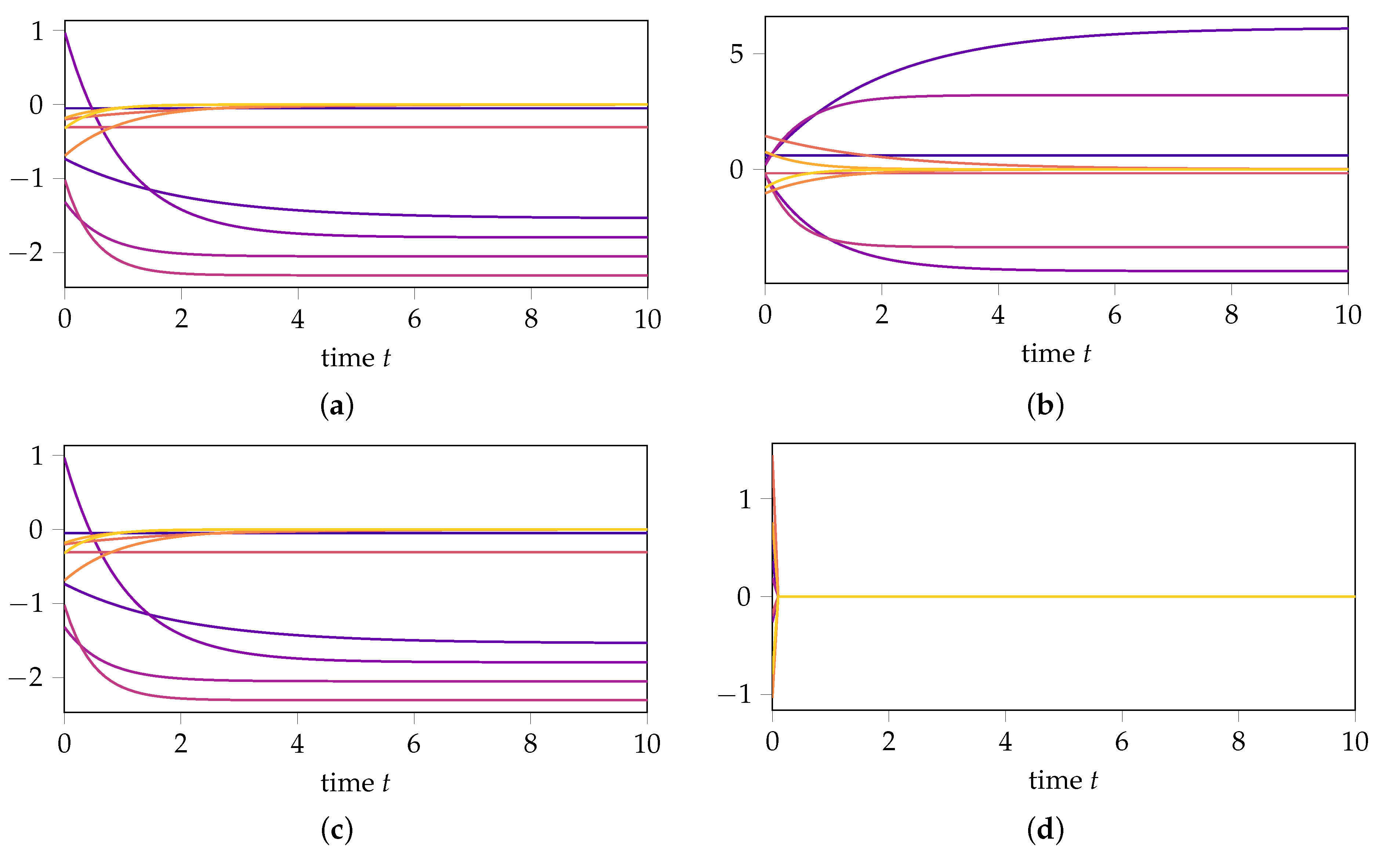
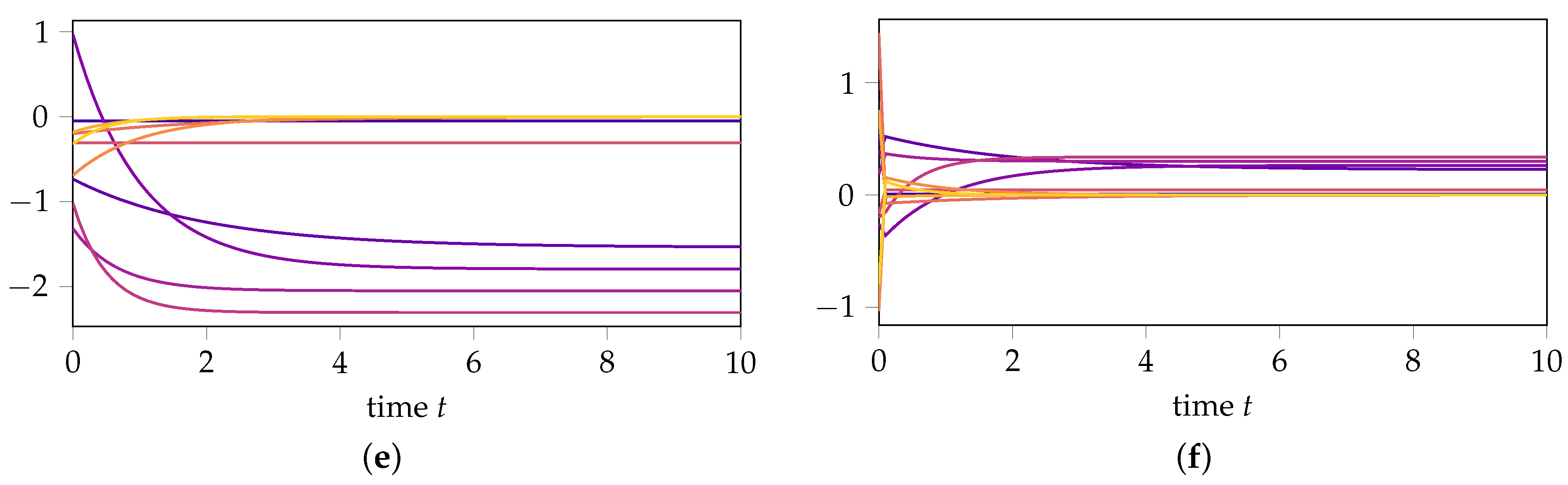
For our numerical experiment, whose results are depicted in Figure 2, we choose the initial values

$${\tilde{x}}_0:=U_{1}e\in span\left(U_1\right)\mathrm{and}{\widehat{x}}_0:=U_{2}e\in span\left(U_2\right)=span{\left(U_1\right)}^{\perp },$$

with $e={[1,1,1,1,1]}^{\top }$. The exact solution for both initial values is presented in Figure 2a,b, respectively. Our simulations confirm the following:

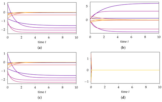
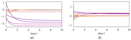
Figure 2. Comparison of the exact solution, DMD approximation, and DMD approximation based on transformed data for initial values inside the reachable subspace, i.e., ${\tilde{x}}_0\in \mathcal{C}(F,x_0)$ and outside the reachable subspace, i.e., ${\widehat{x}}_0\in \mathcal{C}{(F,x_0)}^{\perp }$. (a) Exact solution with initial value ${\tilde{x}}_0$. (b) Exact solution with initial value ${\widehat{x}}_0$. (c) DMD approximation with initial value ${\tilde{x}}_0$. (d) DMD approximation with initial value ${\widehat{x}}_0$. (e) DMD with transformed data with initial value ${\tilde{x}}_0$. (f) DMD with transformed data with initial value ${\widehat{x}}_0$.

• As predicted by Theorem 2, the DMD approximation for the initial value ${\tilde{x}}_0$, depicted in Figure 2c, exactly recovers the exact solution, while the DMD approximation for the initial value ${\widehat{x}}_0$ (cf. Figure 2d) is identically zero.
• If we first transform the data with the matrix

  $$T=\left[\begin{array}{cc}1& 1\\ & \ddots & \ddots \\ & & \ddots & 1\\ & & \phantom{\ddots }& 1\end{array}\right]\in {\mathrm{GL}}_{2N}\left(\mathbb{R}\right),$$

  then compute the DMD approximation, and then transform the results back, the DMD approximation for ${\tilde{x}}_0$ remains unchanged (see Figure 2e), confirming (14) from Theorem 1. In contrast, the prediction of the dynamics for ${\widehat{x}}_0$ changes (see Figure 2f), highlighting that DMD is not invariant under state-space transformations in the orthogonal complement of the data.

The presented numerical example is chosen to illustrate the importance of the reachable space. Computing a subspace numerically is a delicate task in particular if, as in our example, the ratio of the largest and the smallest entry in the controllability matrix is of size $\frac{{(1/2)}^{2N-3}{(N-1)}^{2N}}{{(1/2)}^{2N-1}}=4{(N-1)}^{2N}$, which leads to huge rounding errors already for moderate N. This mainly concerns the separation of the reachable and the unreachable subspace, which, however, can be monitored in a general implementation for a general setup. Since in standard SVD implementations, the dominant directions (and, thus, the Moore–Penrose inverse) are computed with high accuracy, for quantitative approximations using DMD, these numerical issues are less severe.

5. Conclusions

This work highlighted fundamental properties of the DMD approach if applied to linear problems both in continuous and discrete times. Depending on how the initial data relate to the reachable space, the DMD can recover the exact discrete-time dynamics. If, in addition, the discrete-time data are generated from a continuous-time system via time discretization with a Runge–Kutta scheme, then the error of the DMD approximation is in the same order as the time-integration method. As a by-product of our analysis, we made a relation of the Moore–Penrose inverse and regular transformations explicit, which has not been stated so far. Although the findings mainly confirm what should be expected, the basic principles, such as controllability, will well generalize to nonlinear problems.

References

- Benner, P.; Cohen, A.; Ohlberger, M.; Willcox, K. Model Reduction and Approximation; SIAM: Philadelphia, PA, USA, 2017. [Google Scholar] [CrossRef] [Green Version]
- Quarteroni, A.; Manzoni, A.; Negri, F. Reduced Basis Methods for Partial Differential Equations: An Introduction; UNITEXT, Springer: Berlin, Germany, 2016. [Google Scholar] [CrossRef]
- Antoulas, A.C. Approximation of Large-Scale Dynamical Systems; Advances in Design and Control; SIAM: Philadelphia, PA, USA, 2005; p. 489. [Google Scholar]
- Hesthaven, J.S.; Rozza, G.; Stamm, B. Certified Reduced Basis Methods for Parametrized Partial Differential Equations; Springer: Berlin, Germany, 2016. [Google Scholar]
- Antoulas, A.C.; Beattie, C.A.; Güğercin, S. Interpolatory Methods for Model Reduction; SIAM: Philadelphia, PA, USA, 2020. [Google Scholar] [CrossRef]
- Mayo, A.J.; Antoulas, A.C. A framework for the solution of the generalized realization problem. Linear Algebra Appl. 2007, 425, 634–662. [Google Scholar] [CrossRef] [Green Version]
- Beattie, C.; Gugercin, S. Realization-independent H2-approximation. In Proceedings of the 2012 IEEE 51st IEEE Conference on Decision and Control (CDC), Maui, HI, USA, 10–13 December 2012; pp. 4953–4958. [Google Scholar] [CrossRef]
- Gustavsen, B.; Semlyen, A. Rational approximation of frequency domain responses by vector fitting. IEEE Trans. Power Deliv. 1999, 14, 1052–1061. [Google Scholar] [CrossRef] [Green Version]
- Drmač, Z.; Gugercin, S.; Beattie, C. Quadrature-Based Vector Fitting for Discretized H2 Approximation. SIAM J. Sci. Comput. 2015, 37, A625–A652. [Google Scholar] [CrossRef] [Green Version]
- Drmač, Z.; Gugercin, S.; Beattie, C. Vector Fitting for Matrix-valued Rational Approximation. SIAM J. Sci. Comput. 2015, 37, A2345–A2379. [Google Scholar] [CrossRef]
- Peherstorfer, B.; Willcox, K. Data-driven operator inference for nonintrusive projection-based model reduction. Comput. Methods Appl. Mech. Engrg. 2016, 306, 196–215. [Google Scholar] [CrossRef] [Green Version]
- Kutz, J.; Brunton, S.; Brunton, B.; Proctor, J. Dynamic Mode Decomposition; SIAM: Philadelphia, PA, USA, 2016. [Google Scholar]
- Moler, C.; Van Loan, C. Nineteen Dubious Ways to Compute the Exponential of a Matrix, Twenty-Five Years Later. SIAM Rev. 2003, 45, 3–49. [Google Scholar] [CrossRef]
- Mezić, I. Spectral Properties of Dynamical Systems, Model Reduction and Decompositions. Nonlinear Dyn. 2005, 41, 309–325. [Google Scholar] [CrossRef]
- Hairer, E.; Nørsett, S.; Wanner, G. Solving Ordinary Differential Equations I: Nonstiff Problems; Springer Series in Computational Mathematics; Springer: Berlin, Germany, 2008. [Google Scholar]
- Kunkel, P.; Mehrmann, V. Differential-Algebraic Equations. Analysis and Numerical Solution; European Mathematical Society: Zürich, Switzerland, 2006. [Google Scholar]
- Tu, J.H.; Rowley, C.W.; Luchtenburg, D.M.; Brunton, S.L.; Kutz, J.N. On dynamic mode decomposition: Theory and applications. J. Comput. Dyn. 2014, 1, 391–421. [Google Scholar] [CrossRef] [Green Version]
- Golub, G.H.; Van Loan, C.F. Matrix Computations, 3rd ed.; Johns Hopkins University Press: Baltimore, MD, USA, 1996. [Google Scholar]
- Higham, N. Functions of Matrices: Theory and Computation; Other Titles in Applied Mathematics; SIAM: Philadelphia, PA, USA, 2008. [Google Scholar]
Publisher’s Note: MDPI stays neutral with regard to jurisdictional claims in published maps and institutional affiliations. |
© 2022 by the authors. Licensee MDPI, Basel, Switzerland. This article is an open access article distributed under the terms and conditions of the Creative Commons Attribution (CC BY) license (https://creativecommons.org/licenses/by/4.0/).