Robust Stabilization via Super-Stable Systems Techniques

Abstract

In this paper, we propose a direct method for the synthesis of robust systems operating under parametric uncertainty of the control plant model. The developed robust control procedures are based on the assumption that the structural properties of the nominal system are conservated over the entire range of parameter changes. The invariant-to-parametric-uncertainties transformation of the initial model to a regular form makes it possible to use the concept of super-stable systems for the synthesis of a stabilizing feedback. It is essential that the synthesis of super-stable systems is carried out not on the basis of assigning eigenvalues to the matrix of the close-loop system, but in terms of its elements. The proposed approach is applicable to a wide class of linear systems with parametric uncertainties and provides a given degree of stability.

1. Introduction

The problem of stabilizing the state variables of dynamic automatic control plants is a fundamental problem, the formulation and solution of which served as the basis for the formation and development of control theory. Classical methods of control theory, in particular modal control, are based on the assumption of an accurate description of the mathematical model of the control process and the environment of its operation. In reality, there is often parametric uncertainty in the mathematical model of control plants, in particular due to the discarding of residual terms of higher order in the linearized models. This leads to the need to consider a parametrically indeterminate model when synthesizing feedback and to set the robust control problem. Many researchers are currently paying increased attention to control problems in conditions of parametric uncertainty. The direct way to solve the stabilization problem is to obtain estimates of unknown parameters of the control plant model, either directly using the parametric identification theory [1,2], or indirectly, based on the adaptation theory [3,4]. After obtaining estimates of unknown parameters, it becomes possible to use well-developed modal control methods. Another trend in solving the problem of stabilization of parametrically uncertain systems refers to the currently actively developing theory of robust control, in which we can roughly define two main fields: problems of analysis and problems of synthesis. Classical methods for analyzing open-loop systems include results on interval stability of polynomials [5,6], robust frequency methods [7], the D-partition technique [8], $H_{\infty }$ optimization methods [9], and others. Direct and very effective methods of robust control include the use of sliding-mode technique [10] and deep feedback [11]. Note that both methods provide the independence of motions in the sliding mode (slow motions) only from the matching uncertainties. It should be noted that usually on the problem statement step of these approaches, no assumptions are made about the structural properties of the controllability of the system. These methods of robust theory allow us to establish only the fact of system stability and do not give a direct answer to the question of the nature of convergence, which reduces their practical value.

This paper considers a different approach to robust stabilization, where a guaranteed stability margin for linear stationary systems with interval parameter uncertainty is achieved using linear state feedback. The methodological basis of the developed approach is the synthesis of super-stable closed systems [12], and decomposition is based on the transformation of the control plant model to a regular form [13]. It is essential that in these approaches, the results are expressed in terms of matrix elements rather than their eigenvalues. Possibilities for extending this approach are available by using the block approach [14,15,16].

The paper has the following structure. Section 2 considers parametrically certain linear stationary systems. As a methodological basis for further discussion, the procedure of modal synthesis based on transformation to a regular form is presented. For the particular case of a regular form, which consists of two elementary subsystems, we formalize a procedure for the synthesis of a stabilizing feedback that ensures super-stability of the closed-loop system in the new coordinate basis and a guaranteed stability margin in the initial system. Section 3 considers a significant practical class of linear stationary systems, in which, for all values of uncertain parameters from intervals with known bounds, the structural controllability properties defined by the nominal system are conserved. For a class of systems with a controllability indicator equal to two, we formalize rank requirements for the structure of indeterminate matrices, in case of which the indeterminate system is reduced to a regular form regardless of the unknown parameters. Sufficient conditions for the feasibility of robust control are formalized. The procedure for synthesizing a stabilizing feedback is also formalized. In this case, the super-stability of the system is ensured in the coordinate basis of a regular form, and for the original system, a given stability margin is provided in all intervals of uncertain parameters. Section 4 contains numerical examples to illustrate the developed theoretical results.

2. Parametrically Certain Systems

2.1. The Elementary Control Problem

A mathematical model of a linear stationary control plant is considered

$$\dot{x}=Ax+Bu,$$

(1)

where $x\in R^n$ is measurable state vector, $u=\mathrm{col}(u_1,\dots ,u_m)\in R^m$ is control vector; $A\in R^{n\times n},\hspace{0.17em}B\in R^{n\times m}$ are constant known matrices, and pair $(A,\hspace{0.17em}B)$ is controllable.

For system (1), there is a problem of stabilization by means of a linear static feedback

$$u=Fx,$$

(2)

resulting in a closed-loop system

$$\dot{x}=(A+BF)x\hspace{0.17em}=A_{0}x.$$

(3)

Typical for a linear system is the modal control problem, in which the choice of the feedback matrix $F\in R^{m\times n}$ must assign a given spectrum ${\sigma }_{\mathrm{d}}$ to the closed-loop matrix

$${\sigma }_{\mathrm{d}}=\sigma (A_0)=\{{\lambda }_i\in C:\hspace{0.17em}\det \hspace{0.17em}({\lambda }_i{I}_n-A_0)=0,\hspace{0.17em}i=\overline{1,n}\}, \mathrm{Re}{\lambda }_i(A_0)<0,\hspace{0.17em}i=\overline{1,n},$$

(4)

which ensures asymptotic convergence of the state vector to the zero equilibrium position

$$\underset{t\to +\infty }{\lim }x(t)=\overrightarrow{0}.$$

In Formula (4) and below, I is unit matrix of a given dimension.

In general, the following problems arise when solving the modal control problem:

(1)

by assigning only eigenvalues in a closed system (3), it is not always possible to achieve the desired transients of the state variables;

(2)

in multidimensional systems with vector control, there are certain computational difficulties in synthesis, called the “curse of dimensionality”;

(3)

full parametric certainty of the matrices $A$ and $B$ is required.

The first two problems can be solved in some special cases of system (1). These include elementary systems with full-rank control.

Definition 1.

System (1) is called elementary if the number of controls in it is not less than the dimensionality of the state vector and the control matrix has a full rank:

$$\dim u=m\ge n=\dim x, \mathrm{rank}{B}_{n\times m}=n.$$

The synthesis problem in the elementary system is also called elementary, because the feedback matrix is directly found from the matrix equation $A+BF=A_0$, such as

$$m>n:\hspace{0.17em}F=B^{+}(A_0-A);\hspace{0.17em}m=n:\hspace{0.17em}F=B^{-1}(A_0-A),$$

(5)

where in the first expression $B^{+}$—pseudo-inverse matrix $B$, $B{B}^{+}B=B$. In the elementary system, the matrix $B$ rows are linearly independent, hence $B_{n\times m}{B}_{m\times n}^{+}=I_n$ and $B^{+}=B^T{(B{B}^T)}^{-1}$ [17].

Thus, in the elementary system, at first, the synthesis problem (5) is solved in terms of matrix elements rather than their eigenvalues. Second, one can easily provide the desired transients in all state variables by choosing a reference matrix of simple structure, in a Jordanian form or diagonal form. In the latter case, the transient process of each state variable will be monotonous with a given rate of convergence to zero, which is determined by the values of the diagonal elements of the reference matrix.

The advantages of systems with full control are obvious, but in practice, usually the control problem is not elementary. In the next subsection, the procedure of nonsingular linear transformations is given, which allows extracting an elementary subsystem with full control from the initial system of general form.

2.2. Synthesis of Modal Control Based on a Regular Form

We will consider the general case of system (1), where the number of controls is less than the dimension of the state vector and $0<\mathrm{rank}{B}_{n\times m}=m_0\le m<n$, i.e., out of $n$ matrix rows $B$ only $m_0$ are basic. For such a system, there is an equivalent representation in a new coordinate basis, which is called a regular form (RF) with respect to the control [13,18]. In this form, the elementary subsystem with full control is singled out. The point of the corresponding linear nonsingular transformation is grouping of basis rows and zeroing linearly dependent rows of the matrix $B$.

Definition 2.

A regular form with respect to the control vector is an equivalent representation of system (1), $\mathrm{rank}{B}_{n\times m}=m_0\le m<n$ in the form of two subsystems

$$\begin{array}{l}{\dot{x}}_1=A_{11}{x}_1+A_{12}{x}_2,\\ {\dot{x}}_2=A_{21}{x}_1+A_{22}{x}_2+B_{2}u,\end{array}$$

(6)

which are obtained as a result of nonsingular variable change

$$Tx=\overline{x}=\left(\begin{array}{l}{x}_1\\ x_2\end{array}\right), \det T_{(n\times n)}\ne 0,x_1\in R^{n-m_0},\mathrm{rank}B=\mathrm{rank}{B}_2=\dim x_2=m_0$$

and similarity transformation

$$TA{T}^{-1}=\overline{A}=\left(\begin{array}{cc}{A}_{11(n-m_0)\times (n-m_0)}& A_{12(n-m_0)\times m_0}\\ A_{21(m_0\times (n-m_0))}& A_{22(m_0\times m_0)}\end{array}\right),TB=\overline{B}=\left(\begin{array}{l}{O}_{(n-m_0)\times m}\\ B_{2(m_0\times m)}\end{array}\right).$$

Here and further in the text, $O$ is the zero matrix of the corresponding dimension.

The second subsystem of system (6) contains full-rank control, which is a condition for the solution of the elementary control problem in this subsystem; similar to (5), pair $(A_{22},\hspace{0.17em}{B}_2)$ is obviously controllable. In the first subsystem of system (6), which in the general case is not elementary, the vector $x_2$ is considered virtual control action. If system (1) pair $(A,B)$ is controllable, then due to invariance of the controllability property to nonsingular linear transformations, this means that in the first subsystem of (6) the pair $(A_{11},\hspace{0.17em}{A}_{12})$ is also controllable.

Note that there can be several sets of basis rows in matrix $B$, so in general there are several equivalent realizations of the regular form (6) for a particular system. They differ by the values of the matrix elements $\overline{A}$ and $B_2$, but all have the same structure, in that the first subsystem has no control, and the second has a dynamic order $m_0$ and is elementary.

Based on the regular form, the problem of synthesis of modal control is decomposed into two successively solvable subproblems of lesser dimensions than the original system. In the first subsystem $n-m_0$ with virtual control $x_2$, the problem of assigning a part of a given spectrum (4) is solved. The derived linear local feedback is introduced by a nonsingular linear transformation, and the assignment of the second part of the spectrum is provided by a real linear control $u$, meaning the elementary synthesis problem of dimension $m_0$ is solved. As a result, a linear control law for the variables of the transformed system will be obtained. Using the resulting transformation matrix, it should be presented with respect to the state variables of the initial system in the form (2). According to the property of invariance of the roots of the characteristic equation to nondegenerate linear transformations, the characteristic polynomials (and hence the spectrum) of matrices of closed-loop initial and transformed systems will be equal to each other. Let us present these transformations in the form of a step-by-step description.

Procedure 1.

Synthesis of modal control based on transition to a regular form.

• Nonsingular transformation of system (1) to the regular form (6).

1.a. Grouping basis rows of the matrix $B$ and forming matrix $B_{2(m_0\times m)}$.

If necessary, rearrange the matrix $B$ rows in a way that $m_0$ of its last rows are linearly independent, and perform an appropriate variable change, in which the transformation matrix is a permutation matrix $T_{p(n\times n)}$, $\det T_p\ne 0$:

$$\begin{gathered} T_{p}B=\tilde{B}=\left(\begin{array}{l}{\tilde{B}}_1\\ B_2\end{array}\right),T_{p}x=\tilde{x}=\left(\begin{array}{l}{\tilde{x}}_1\\ x_2\end{array}\right),{\tilde{x}}_1\in R^{n-m_0},T_{p}A{T}_p^{-1}=\tilde{A}=\left(\begin{array}{cc}{\tilde{A}}_{11}& {\tilde{A}}_{12}\\ {\tilde{A}}_{21}& {\tilde{A}}_{22}\end{array}\right), \\ \mathrm{rank}B=\mathrm{rank}{B}_2=\dim x_2=m_0. \end{gathered}$$

(7)

System (1) will be represented in the following equivalent form:

$${\dot{\tilde{x}}}_1={\tilde{A}}_{11}{\tilde{x}}_1+{\tilde{A}}_{12}{x}_2+{\tilde{B}}_{1}u, \hspace{0.17em}{\dot{x}}_2={\tilde{A}}_{21}{\tilde{x}}_1+{\tilde{A}}_{22}{x}_2+B_{2}u.$$

(8)

If no permutations are required, then $T_p=I$, and to obtain the system (8), the appropriate notation is introduced.

1.b. Zeroing out the linearly dependent rows of a matrix $B$.

If in system (8) ${\tilde{B}}_{1(n-m_0)\times m}\ne O$, then the matrix ${\tilde{B}}_1$, which consists of linearly dependent rows of a matrix $B_2$, needs to be reset to zero. It is required that as a result of partial change of the variables,

$$x_1={\tilde{x}}_1-B_2^{\ast }{x}_2,\hspace{0.17em}{x}_1\in R^{n-m_0}.$$

(9)

In the new subsystem relative to $x_1$ control was absent, as follows

$${\dot{x}}_1={\dot{\tilde{x}}}_1-B_2^{\ast }{\dot{x}}_2=({\tilde{A}}_{11}-B_2^{\ast }{\tilde{A}}_{21}){\tilde{x}}_1+({\tilde{A}}_{12}-B_2^{\ast }{\tilde{A}}_{22})x_2+({\tilde{B}}_1-B_2^{\ast }{B}_2)u\Rightarrow {\tilde{B}}_1-B_2^{\ast }{B}_2=O.$$

From the resulting matrix equation, we have

$$m_0<m:B_2^{\ast }={\tilde{B}}_1{B}_{2(m\times m_0)}^{+},\hspace{0.17em}{B}_2^{+}=B_2^T{(B_2{B}_2^T)}^{-1};\hspace{0.17em}{m}_0=m:\hspace{0.17em}{B}_2^{\ast }={\tilde{B}}_1{B}_{2(m\times m)}^{-1}.$$

(10)

The corresponding transformation of partial variable change (9) has the form

$$\begin{gathered} T_a\tilde{B}=T_a\left(\begin{array}{l}{\tilde{B}}_1\\ B_2\end{array}\right)=\overline{B}=\left(\begin{array}{l}O\\ B_2\end{array}\right),\det T_{a(n\times n)}\ne 0, T_a\tilde{x}=T_a\left(\begin{array}{l}{\tilde{x}}_1\\ x_2\end{array}\right)=\overline{x}=\left(\begin{array}{l}{x}_1\\ x_0\end{array}\right),T_a\tilde{A}{T}_a^{-1}=\overline{A} \\ , T_a=\left(\begin{array}{ll}\hspace{0.17em}{I}_{n-m_0}& -B_{2(n-m_0)\times m_0}^{\ast }\\ O_{m_0\times (n-m_0)}& I_{m_0}\end{array}\right),T_a^{-1}=\left(\begin{array}{cc}{I}_{n-m_0}& B_{2(n-m_0)\times m_0}^{\ast }\\ O_{m_0\times (n-m_0)}& I_{m_0}\end{array}\right) \end{gathered}$$

(11)

and leads system (8) to the regular form (6). If in system (8) ${\tilde{B}}_{1(n-m_0)\times m}=O$, it corresponds exactly to the regular form (6) and $T_a=I$.

The sequence of the above transformations of system (1) to the regular form (6) is

$$Tx=T_a(T_{p}x)=\overline{x},\hspace{0.17em}T=T_a{T}_p,$$

(12)

where some cases may be $T_p=I$ and/or $T_a=I$. Clearly, the equality $T_p=T_a=I$ occurs in mathematical models that are initially of the regular form (6), and this situation is typical of many practical applications.

Procedure 2.

Decomposition synthesis of modal control based on RF.

2.a. Synthesis of fictitious control in the first RF subsystem.

We have to choose $n-m_0$ values from a given spectrum ${\sigma }_d$ (4) so as not to disconnect complex-conjugate pairs, if any. If an odd $n-m_0$ and/or $m_0$ is required to break the complex-conjugate pair, then the decomposition will have to be dropped, and a different synthesis method should be used. Otherwise, this method will produce a complex feedback matrix (2), which is not acceptable in practical applications.

If the above choice is possible, in the first subsystem of system (6) we form a linear virtual control $x_2=F_1{x}_1$ and obtain the local feedback matrix

$$F_{1(m_0\times (n-m_0))}:A_1=A_{11}+A_{12}{F}_1,\sigma (A_1)\subset {\sigma }_{\mathrm{d}}.$$

(13)

Due to the controllability of the pair $(A_{11},\hspace{0.17em}{A}_{12})$, this problem has a solution. In the particular case $\mathrm{rank}{A}_{12}=\dim x_1=n-m_0\le m_0$, when also the first subsystem is elementary, then similarly to (5) we can assign in it both a given spectrum and a given matrix of own movements. In the general case, problem (13) is not elementary, but the dimensions of the desired matrix are smaller than when solving problem (3) in the original system (1), (2), where $\dim F=m\times n.$

Remark 1.

In many applications, the transition to the RF simplifies the synthesis procedure sufficiently, and it is possible to simply represent the initial system in the form of two subsystems. In general case for large-dimensional systems, one can continue the mentioned transformations and in the first subsystem of (6) allocate in a similar way an elementary subsystem with respect to virtual control $x_2$, etc. As a result, the first subsystem of system (6) will be represented as associated elementary subsystems (blocks) with full-rank virtual controls, which are the variables of the following block. The form in this case is called the block form of controllability, on the basis of which the synthesis problem is divided into consecutive elementary control problems [14].

In order to implement the local relation of variables that has been formed, we need to introduce a mismatch between the real control and the selected virtual control by means of partial variable change

$$x_2=F_1{x}_1, e_1:=x_1,\hspace{0.17em}{e}_2=x_2-F_1{x}_1,\hspace{0.17em}{e}_2\in R^{m_0}$$

(14)

and the corresponding linear transformation

$$\begin{gathered} T_e\overline{x}=\left(\begin{array}{l}{x}_1\\ x_2\end{array}\right)=e=\left(\begin{array}{l}{e}_1\\ e_2\end{array}\right), T_e=\left(\begin{array}{l}\hspace{0.17em}{I}_{(n-m)}\hspace{0.17em}\hspace{0.17em}\hspace{0.17em}\hspace{0.17em}\hspace{0.17em}\hspace{0.17em}\hspace{0.17em}\hspace{0.17em}\hspace{0.17em}{O}_{(n-m_0)\times m_0}\\ -F_{1(m_0\times (n-m_0))}\hspace{0.17em}\hspace{0.17em}\hspace{0.17em}\hspace{0.17em}\hspace{0.17em}\hspace{0.17em}\hspace{0.17em}\hspace{0.17em}{I}_{m_0}\end{array}\right),T_e^{-1}=\left(\begin{array}{l}\hspace{0.17em}{I}_{(n-m_0)}\hspace{0.17em}\hspace{0.17em}\hspace{0.17em}\hspace{0.17em}\hspace{0.17em}{O}_{(n-m_0)\times m_0}\\ F_{1(m_0\times (n-m_0))}\hspace{0.17em}\hspace{0.17em}\hspace{0.17em}\hspace{0.17em}\hspace{0.17em}\hspace{0.17em}\hspace{0.17em}\hspace{0.17em}{I}_{m_0}\end{array}\right), \\ \det T_{e(n\times n)}\ne 0,T_e\overline{A}{T}_e^{-1}=A_e=\left(\begin{array}{l}{A}_1\hspace{0.17em}\hspace{0.17em}\hspace{0.17em}{A}_{12}\\ C_{21}\hspace{0.17em}\hspace{0.17em}{C}_{22}\end{array}\right),T_e\overline{B}=T_e\left(\begin{array}{l}O\\ B_2\end{array}\right)=\left(\begin{array}{l}O\\ B_2\end{array}\right). \end{gathered}$$

(15)

As a result, RF with local relation closed-loop will be obtained:

$$\begin{array}{l}{\dot{e}}_1=A_1{e}_1+A_{12}{e}_2,\\ {\dot{e}}_2=C_{21}{e}_1+C_{22}{e}_2+B_{2}u.\end{array}$$

(16)

2.b. Synthesis of real control by variables of transformed systems.

Next, the local feedback generated in the first subsystem of (16) must be provided by the real control. For the second elementary subsystem of (16) we have to compose a reference matrix $A_{2(m_0\times m_0)}$ with $m_0$ with eigenvalues from the rest of the given spectrum $\sigma (A_1)\cup \sigma (A_2)={\sigma }_{\mathrm{d}}$, and form a feedback on the variables of the transformed system:

$$\begin{array}{l}{m}_0<m:\hspace{0.17em}\hspace{0.17em}u=B_2^{+}(-C_{21}{e}_1-C_{22}{e}_2+A_2{e}_2)=Ke;\\ m_0=m:\hspace{0.17em}\hspace{0.17em}u=B_2^{-1}(-C_{21}{e}_1-C_{22}{e}_2+A_2{e}_2)=Ke.\hspace{0.17em}\hspace{0.17em}\end{array}$$

(17)

System (16), with closed-loop by control (17), will take the form

$${\dot{e}}_1=A_1{e}_1+A_{12}{e}_2,\hspace{0.17em}\hspace{0.17em}\hspace{0.17em}{\dot{e}}_2=A_2{e}_2.$$

(18)

Its matrix has an upper triangular block structure

$$\left(\begin{array}{l}{A}_1\hspace{0.17em}\hspace{0.17em}\hspace{0.17em}\hspace{0.17em}{A}_{12}\\ O\hspace{0.17em}\hspace{0.17em}\hspace{0.17em}\hspace{0.17em}\hspace{0.17em}\hspace{0.17em}\hspace{0.17em}{A}_2\end{array}\right)$$

and is stable according to (4), and its eigenvalues meet the characteristic equation $\det (\lambda I-A_1)\det (\lambda I-A_2)=0$.

2.c. A modal control law based on the state of the initial system.

Finally, based on (17), it is necessary to form a feedback on the variables of the original systems (1) and (2), since it is these variables that are measured. By substitutions of variables (7), (11), and (15), the resulting transformation matrix and the resulting modal control law (2) are as follows:

$$T_e{T}_a{T}_{p}x=e, u=Ke=Fx,F_{m\times n}=K{T}_e{T}_a{T}_p,$$

(19)

which provides (3), (4), and a solution to the stabilization problem.

Modal control synthesis is complete.

As stated in subsection 2.a, full parametric certainty of the matrices $A$ and $B$ is required to implement modal control, which limits its applicability in practical applications, as models of real-world control plants often depend on unknown parameters.

In such cases, the requirements of the closed-loop system are relaxed, and the stability margin, which is one of the key quality indicators of the transition process, is considered as the target condition. The problem is to synthesize a linear feedback (2), which provides in the closed-loop system (3) a stability margin not less than a given ${\eta }_{\mathrm{d}}>0$:

$$\min {\{-\mathrm{Re}{\lambda }_i(A+BF)\}}_{i=\overline{1,n}}=\eta \ge {\eta }_{\mathrm{d}}.$$

(20)

As a methodological basis for problem (20), we will use the concept of super-stability of the system, which is defined in terms of matrix elements using inequalities rather than characteristic Equation (4), which is a precondition for using this concept in solving robust control problems in systems with uncertain parameters.

Definition 3

([12]). Matrix $A=(a_{ij})\in R^{n\times n}$ and, consequently, the system $\dot{x}=Ax$ are called super-stable if $A$ is a negative-diagonal-dominated matrix, i.e., all the elements of its main diagonal are negative numbers $a_{ii}<0,\hspace{0.17em}i=\overline{1,\hspace{0.17em}n}$, which are greater in absolute value than the sum of the modules of the non-diagonal elements in the row:

$$\min {\{-a_{ii}-{\displaystyle \sum _{j=1,\hspace{0.17em}j\ne i}^n\left|a_{ij}\right|}\}}_{i=\overline{1,n}}=\nu >0,$$

(21)

where $\nu$ has the meaning of a margin of super-stability.

The statements in Lemma 1 below are rather obvious. However, we will present a rigorous proof of them, because they are important for further discussion.

Lemma 1.

Any super-stable matrix $A=(a_{ij})\in R^{n\times n}$, (21) is Hurwicz, and its stability margin$\min {\{-\mathrm{Re}{\lambda }_i(A)\}}_{i=\overline{1,n}}=\eta >0$is as much as the margin of her super-stability (21), i.e.,

$$\eta \ge \nu .$$

(22)

Proof 1.

According to Gershgorin’s theorem [17], each of the eigenvalues $\lambda$ of matrix $A$ is always located in one of the circles of the complex plane $\left|a_{ii}-\lambda \right|\le {\displaystyle \sum _{j=1,j\ne i}^n\left|a_{ij}\right|}$, $i=\overline{1,\hspace{0.17em}n}$ centered at $a_{ii}$ and with a radius of ${\displaystyle \sum _{j=1,j\ne i}^n\left|a_{ij}\right|}$. Each eigenvalue $\lambda$ of matrix $A$ corresponds to the eigenvector $h$: ${\displaystyle \sum _{j=1}^n{a}_{ij}h=\lambda h}$, $i=\overline{1,\hspace{0.17em}n}$. Let $\left|h_k\right|=\underset{i}{\max }\left|h_i\right|>0$; then,

$$\left|a_{kk}-\lambda \right|\left|h_k\right|=\left|{\displaystyle \sum _{i,j\ne k}^n{a}_{kj}{h}_i}\right|\le \left|h_k\right|{\displaystyle \sum _{j\ne k}^n\left|a_{kj}\right|} \mathrm{and} \left|a_{kk}-\lambda \right|\le {\displaystyle \sum _{j\ne k}^n\left|a_{kj}\right|}.$$

It follows that if the matrix $A$ is super-stable and $-a_{kk}>{\displaystyle \sum _{j\ne k}^n\left|a_{kj}\right|}$, then each of its eigenvalues lies in the left half-plane of the complex plane, i.e., matrix $A$ is Hurwitz and its stability margin is defined as $\eta =-\mathrm{Re}{\lambda }_0=\min \{-\mathrm{Re}{\lambda }_i(A)\}>0$.

Let ${\lambda }_0$ be a real simple eigenvalue of the matrix $A$, to which corresponds the eigenvector ${\overline{h}}_0={(h_1,\dots ,h_n)}^T$, ${\lambda }_0{\overline{h}}_0=A{\overline{h}}_0$, and for the $k$-th ($k=1,2,\dots ,n$) element we have: ${\lambda }_0{h}_k={\displaystyle \sum _{j=1}^n{a}_{kj}{h}_j}$. Let $h_k$ be an element with a maximum module ${\overline{h}}_0$: $\left|h_k\right|=\max {\left\{\left|h_i\right|\right\}}_{i=\overline{1,n}}$. Then, a fair estimate is $\left|{\lambda }_0\right|\left|h_k\right|\ge \left|a_{kk}\right|\left|h_k\right|-{\displaystyle \sum _{j=1,j\ne k}^n\left|a_{kj}\right|}|h_j|\ge \left|h_k\right|(\left|a_{kk}\right|-{\displaystyle \sum _{j=1,j\ne k}^n\left|a_{kj}\right|})=\left|h_k\right|\nu$, whence it follows $\eta =\left|{\lambda }_0\right|\ge \nu$, inequality (20) is satisfied. The case of $\mathrm{Re}{\lambda }_0$ corresponds to a pair of complex-conjugate eigenvalues, and the estimate becomes $\left|\mathrm{Re}{\lambda }_0\right|\left|h_k\right|\ge \left|a_{kk}\right|\left|h_k\right|-{\displaystyle \sum _{j=1,j\ne k}^n\left|a_{kj}\right|}\left|h_j\right|\ge \left|h_k\right|\nu$ inequality (26) is satisfied.

In the case of an multiple-eigenvalue ${\lambda }_0$, similar estimates hold for all linearly independent eigenvectors corresponding to a given eigenvalue. Lemma 1 is proved. □

In a controllable linear system with certain parameters, it is always possible to achieve stability with state feedback, but super-stability is rarely achieved due to a lack of control actions. In this sense, the only obvious exceptions are elementary systems.

As it is shown in subsection 2.a, it is possible to provide any reference matrix $A_0$, including a super-stable one, in a closed-loop system using feedback (2) and (5), if the parameters of the elementary system are known. Let us note that a diagonal matrix with negative elements $A_0=\mathrm{diag}\left\{a_i\right\}$, $a_i<0,\hspace{0.17em}i=\overline{1,\hspace{0.17em}n}$ is a special case of a super-stable matrix, where $\min \left\{\left|a_i\right|\right\}=\min \{-{\lambda }_i(A_0)\}=\eta =\nu$.

Let us distinguish a class of nonelementary linear systems, for the stabilization of which with a given stability margin (20) we can interconnectively apply the concept of super-stability and decomposition synthesis based on the transition to the RF. This class includes a particular case of controllable systems (1), in which RF (6) will consist of two elementary subsystems. The possibility of such a representation is contained in the rank structure of the controllability matrix.

If system (1), where $0<\mathrm{rank}{B}_{n\times m}=m_0\le m<n$, is controllable, its controllability matrix is of full rank:

$$\mathrm{rank}{(B\hspace{0.17em}\hspace{0.17em}\hspace{0.17em}AB\hspace{0.17em}\hspace{0.17em}\hspace{0.17em}{A}^{2}B\hspace{0.17em}\hspace{0.17em}\hspace{0.17em}\dots \hspace{0.17em}\hspace{0.17em}\hspace{0.17em}{A}^{n-m_0}B)}_{n\times m(n-m_0+1)}=n.$$

(23)

The rank structure of the controllability matrix (23) is characterized by a controllability index and a controllability indicator [19]. If the rank of the controllability matrix (23) is increased according to the following scheme:

$$\begin{gathered} \mathrm{rank}B=m_0\ne 0, \mathrm{rank}(B\hspace{0.17em}\hspace{0.17em}\hspace{0.17em}AB)=m_0+m_1, m_0\ge m_1\ne 0, \\ \mathrm{rank}(B\hspace{0.17em}\hspace{0.17em}\hspace{0.17em}AB\hspace{0.17em}\hspace{0.17em}\hspace{0.17em}\hspace{0.17em}{A}^{2}B)=m_0+m_1+m_2, m_1\ge m_2\ne 0,\text{…}, \\ \mathrm{rank}(B\hspace{0.17em}\hspace{0.17em}\hspace{0.17em}AB\hspace{0.17em}\hspace{0.17em}\dots \hspace{0.17em}\hspace{0.17em}{A}^{r}B)=m_0+m_1+\dots +m_r, m_{r-1}\ge m_r\ne 0, \\ \mathrm{rank}(B\hspace{0.17em}\hspace{0.17em}\hspace{0.17em}AB\hspace{0.17em}\hspace{0.17em}\dots \hspace{0.17em}\hspace{0.17em}{A}^{r}B\hspace{0.17em}\hspace{0.17em}\hspace{0.17em}{A}^{r+1}B)=m_0+m_1+\dots +m_r+0\Rightarrow \\ \Rightarrow \mathrm{rank}(B\hspace{0.17em}\hspace{0.17em}\hspace{0.17em}AB\hspace{0.17em}\hspace{0.17em}\dots \hspace{0.17em}\hspace{0.17em}{A}^{r+1}B\hspace{0.17em}\hspace{0.17em}\hspace{0.17em}{A}^{r+2}B)=m_0+m_1+\dots +m_r+0+0, \end{gathered}$$

(24)

then pair $(A,\hspace{0.17em}\hspace{0.17em}B)$ corresponds to a specific set of natural numbers $m_0,\dots ,m_r$:

$$\mathrm{rank}(B\hspace{0.17em}\hspace{0.17em}\hspace{0.17em}AB\hspace{0.17em}\hspace{0.17em}\hspace{0.17em}\dots \hspace{0.17em}\hspace{0.17em}\hspace{0.17em}{A}^{r}B)=m_0+m_1+\dots +m_r=n, m_0\ge m_1\ge \dots \ge m_r, r\le n-m_0,$$

(25)

which are called the indexes of controllability of the pair $(A,\hspace{0.17em}\hspace{0.17em}B)$. $m_i\in N$, $i=\overline{0,r}$ is the number of linearly independent matrix columns $A^{i}B$, which form the basis of the controllability matrix, compiled according to the specified scheme; $r+1$ is controllability indicator of pair $(A,\hspace{0.17em}\hspace{0.17em}B)$, the number of its controllability indices. □

Lemma 2.

If the controllability matrix of a linear controlled system (1) has a controllability indicator equal to two,

$$\mathrm{rank}{B}_{(n\times m)}=m_0\ne 0, \mathrm{rank}(B\hspace{0.17em}\hspace{0.17em}\hspace{0.17em}AB{)}_{n\times 2m}=m_0+m_1=n, m_0\ge (n-m_0),$$

(26)

then, using the nondegenerate replacement of variables (12), system (1) will be represented in RF (6), in which not only the second, but also the first subsystem will be elementary with respect to the virtual control,

$$\mathrm{rank}{A}_{12(n-m_0)\times m_0}=n-m_0.$$

(27)

Proof 2.

Let us rearrange the blocks of the controllability matrix (26) without performing a rearrangement inside the blocks $W_{(n\times 2m)}=(AB\hspace{0.17em}\hspace{0.17em}B)$. For convenience, we denote $AB=P$. Let us multiply this matrix from the left by the transition matrix to RF (12). According to (7) and (12), the matrix obtained as a result of multiplication can be represented in the following form:

$$TW=T_a{T}_p(P\hspace{0.17em}\hspace{0.17em}\hspace{0.17em}B)=T_a\left(\begin{array}{cc}{\tilde{P}}_1& {\tilde{B}}_1\\ {\tilde{P}}_2& B_2\end{array}\right)=\left(\begin{array}{cc}{P}_{1(n-m_0)\times m}& O\\ P_2& B_{2(m_0\times m)}\end{array}\right)=\overline{W},$$

where $P_1={\tilde{P}}_1-{\tilde{B}}_1{B}_2^{+}{\tilde{P}}_2$. By design, $\mathrm{rank}{W}_{(n\times 2m)}=n,$ and $\mathrm{rank}B=\mathrm{rank}{B}_{2(m_0\times m)}=m_0$. When multiplied by the nonsingular matrix $\det T_{(n\times n)}\ne 0$, the rank does not change and $\mathrm{rank}{\overline{W}}_{(n\times 2m)}=n,$ which is why matrix $P_1$ is of full rank:

$$\mathrm{rank}{P}_{1(n-m_0)\times m}=n-m_0.$$

(28)

Considering that the matrices $W_{n\times 2m}$ and ${\overline{W}}_{n\times 2m}=TW$ are of full rank and consist of linearly independent rows, there are pseudo-inverse matrices for them, and

$$W_{2m\times n}^{+}:\hspace{0.17em}\hspace{0.17em}W{W}^{+}=I_n, {\overline{W}}^{+}={(TW)}^{+}=\left(\begin{array}{cc}{P}_{1(m\times (n-m_0))}^{+}& O\\ \times & B_{2(m\times m_0)}^{+}\end{array}\right).$$

(29)

In Formula (29) and further in the text, the symbol $\times$ denotes matrices, the type of which does not affect the structural properties.

Taking (27) into account, the similarity transformation of the matrix $A$ to RF $TA{T}^{-1}=\overline{A}$ can be represented as

$$TA{T}^{-1}=T\hspace{0.17em}AW{W}^{+}\hspace{0.17em}{T}^{-1}=T\hspace{0.17em}AW{(TW)}^{+}=(TAW){\overline{W}}^{+},$$

where $TAW=TA(AB\hspace{0.17em}\hspace{0.17em}\hspace{0.17em}B)=T(A^{2}B\hspace{0.17em}\hspace{0.17em}\hspace{0.17em}\hspace{0.17em}AB)$, $AB=P$. Then,

$$TA{T}^{-1}=(T(A^{2}B\hspace{0.17em}\hspace{0.17em}\hspace{0.17em}\hspace{0.17em}AB)){\overline{W}}^{+}=\left(\begin{array}{cc}\times & P_1\\ \times & \times \end{array}\right)\left(\begin{array}{cc}{P}_1^{+}& O\\ \times & B_2^{+}\end{array}\right)=\left(\begin{array}{cc}\times & P_1{B}_2^{+}\\ \times & \times \end{array}\right)=\left(\begin{array}{cc}{A}_{11}& A_{12(n-m_0)\times m_0}\\ A_{21}& A_{22}\end{array}\right),$$

where $A_{12(n-m_0)\times m_0}={(P_1{B}_2^{+})}_{(n-m_0)\times m_0}$ due to (28), (29), and $\mathrm{rank}{(P_1{B}_2^{+})}_{(n-m_0)\times m_0}=n-m_0,$ so equality (27) is satisfied. Lemma 2 is proved. □

Let us extend (without proof) the results of Lemma 2 to controlled systems of general form (25).

A consequence of Lemma 2 is as follows. If condition (25) is satisfied in system (1), then it can be represented in the block form of controllability, which consists of $r+1$ elementary blocks of dimension $m_0,\hspace{0.17em}{m}_1,\hspace{0.17em}\dots m_r$ by a linear nonsingular transformation $Tx=(x_1,\hspace{0.17em}\hspace{0.17em}\dots ,\hspace{0.17em}{x}_{r+1}),\hspace{0.17em}\det T\ne 0,$ $x_1\in R^{m_r},\hspace{0.17em}{x}_2\in R^{m_{r-1}},\hspace{0.17em}\dots ,\hspace{0.17em}{x}_{r+1}\in R^{m_0}.$ Matrix $T$ can be found by transforming the matrix $W$ to the bottom-triangular block form with matrices of full rank on the main diagonal:

$$TW=T(A^{r}B\hspace{0.17em}\dots \hspace{0.17em}AB\hspace{0.17em}B)=\overline{W}=\left(\begin{array}{lllll}{P}_r\hfill & \dots \hfill & O\hfill & O\hfill & O\hfill \\ \dots \hfill & \dots \hfill & \dots \hfill & \dots \hfill & \dots \hfill \\ \hfill & \dots \hfill & P_2\hfill & O\hfill & O\hfill \\ \hfill & \dots \hfill & \hfill & P_1\hfill & O\hfill \\ \hfill & \dots \hfill & \hfill & \hfill & P_0\hfill \end{array}\right),\hspace{0.17em}$$

(30)

where $\mathrm{rank}{P}_{0(m_0\times m)}=m_0,$ $\mathrm{rank}{P}_{i(m_i\times m_{i-1})}=m_i,\hspace{0.17em}i=\overline{1,\hspace{0.17em}r}.$

Just as in the procedure of converting to the RF (6), the essence of the transformations is that successively in each block $B,\hspace{0.17em}AB,\hspace{0.17em}\dots ,\hspace{0.17em}\hspace{0.17em}{A}^{r-1}B$, one needs to group $m_i$ basis rows of matrix $P_i$ by transpositions (similar to (7)) and zero out the top linearly dependent lines (similar to (11)). In this case, the leftmost block $A^{r}B$ can be discarded, since its elements do not participate in the formation of the matrix $T$.

For the selected class of systems (1), (26), it is possible to provide a guaranteed stability margin (24) by providing super-stability of the closed system (18) in a new coordinate basis, where the reference matrices $A_1,\hspace{0.17em}{A}_2$ can be assigned arbitrarily. Selecting these matrices diagonally

$$A_1=\mathrm{diag}{\left\{a_i^1\right\}}_{i=\overline{1,\hspace{0.17em}n-m_0}},\hspace{0.17em}{A}_2=\mathrm{diag}{\left\{a_i^2\right\}}_{i=\overline{1,\hspace{0.17em}{m}_0}},$$

(31)

on the one hand, excludes the presence of complex-conjugate eigenvalues in the matrix of the closed system, but, on the other hand, simplifies the computational aspect of the synthesis. Then, for any parameters satisfying the non-strict inequalities

$$\nu \ge {\eta }_{\mathrm{d}},\hspace{0.17em}\hspace{0.17em}{a}_i^1\le -(\nu +{\displaystyle \sum _{j=1}^{m_0}\left|a_{ij}^{12}\right|}),\hspace{0.17em}\hspace{0.17em}{A}_{12}=(a_{ij}^{12}),\hspace{0.17em}\hspace{0.17em}\hspace{0.17em}i=\overline{1,\hspace{0.17em}n-m_0};\hspace{0.17em}\hspace{0.17em}{a}_i^2\le -\nu >0,\hspace{0.17em}i=\overline{1,m_0},$$

(32)

the closed-loop system (18) will be super-stable with a margin of super-stability $\nu \ge {\eta }_{\mathrm{d}}.$

As it was noted, the property of super-stability is formulated in terms of matrix elements (21) rather than their eigenvalues, so it is not invariant to linear transformations, and the initial closed system (1), (19), (31), (32) in general case will not be super-stable. However, because of (22), it guarantees stabilization with a stability margin at least equal to the one given in (20).

In the next section, we consider the possibility of synthesis of robust control of parametrically uncertain systems in the context of the proposed approach.

3. Parametrically Uncertain Systems

3.1. Elementary Control Problem

This section considers the problem of stabilization of linear stationary systems operating under interval parameter uncertainty

$$\dot{x}=(A+\hat{A})x+(B+\hat{B})u, x \in R^n, u \in R^m, m \text{<} n,$$

(33)

where matrices elements $A=(a_{ij}),\hspace{0.17em}\hspace{0.17em}i,j=\overline{1,n}$, $B=(b_{ij})$, $i=\overline{1,n}$, $j=\overline{1,m}$, which define the nominal system (1), are known, and pair $(A,\hspace{0.17em}B)$ is controllable. Elements of matrices $\widehat{A}=({\widehat{a}}_{ij})$ and $\widehat{B}=({\widehat{b}}_{ij})$ are constant but unknown; their values belong to closed intervals with known boundaries:

$$a_{ij\min }\le {\widehat{a}}_{ij}\le a_{ij\max }, \hspace{0.17em}i,j=\overline{1,n}; b_{ij\min }\le {\widehat{b}}_{ij}\le b_{ij\max }, i=\overline{1,n}, j=\overline{1,m}.$$

In the following, to simplify the explanation, we will assume that the values of the uncertain elements are in intervals symmetric with respect to zero

$$a_{ij}-{\stackrel{⌢}{a}}_{ij}\le a_{ij}+{\widehat{a}}_{ij}\le a_{ij}+{\stackrel{⌢}{a}}_{ij}, i,j=\overline{1,\hspace{0.17em}n};\hspace{0.17em}{b}_{ij}-{\stackrel{⌢}{b}}_{ij}\le b_{ij}+{\widehat{b}}_{ij}\le b_{ij}+{\stackrel{⌢}{b}}_{ij}, i=\overline{1,n}, j=\overline{1,m}.$$

(34)

Then, the values of the matrix elements of the system (33) will be in closed intervals with known bounds, symmetrical for the corresponding nominal values

$$a_{ij}-{\stackrel{⌢}{a}}_{ij}\le a_{ij}+{\widehat{a}}_{ij}\le a_{ij}+{\stackrel{⌢}{a}}_{ij}, i,j=\overline{1,\hspace{0.17em}n};\hspace{0.17em}{b}_{ij}-{\stackrel{⌢}{b}}_{ij}\le b_{ij}+{\widehat{b}}_{ij}\le b_{ij}+{\stackrel{⌢}{b}}_{ij}, i=\overline{1,n}, j=\overline{1,m}.$$

It is supposed that pair $((A+\widehat{A}),\hspace{0.17em}(B+\widehat{B}))$ is controllable in all acceptable intervals of parameter uncertainty, and moreover, the rank structures of the controllability matrices of the nominal system (1) and the parametrically perturbed system (33) are the same. This requirement is due to practical considerations. The uncertain system model (33) describes the functioning of a real control plant, and, for example, the failure to meet the condition $\mathrm{rank}\hspace{0.17em}B=\mathrm{rank}\hspace{0.17em}(B+\widehat{B})$ indicates a “faulty” actuator or damaged communication with the control plant.

In a general case, the solution of the modal control problem with the assignment of a given spectrum (4) in the system (33) is not possible. We set the problem of synthesis of linear feedback (2), providing stabilization of the system (33) at all acceptable values of uncertain parameters (34) with stability margin not less than the given one ${\eta }_{\mathrm{d}}>0$, i.e., providing in a closed-loop system

$$\min {\{-\mathrm{Re}{\lambda }_i[(A+\widehat{A})+(B+\widehat{B})F]\}}_{i=\overline{1,n}}=\eta \ge {\eta }_{\mathrm{d}}.$$

(35)

We first investigate the possibility of solving the problem (35) for parametrically uncertain elementary systems of two types. The first type of the considered elementary systems are the systems with known control matrix

$$\dot{x}=(A+\widehat{A})x+Bu,\hspace{0.17em}\hspace{0.17em}\dim u=m\ge n=\dim x=\mathrm{rank}B,$$

(36)

which are obviously controllable. No additional requirements are imposed on them. Variable states with uncertain coefficients cannot be compensated for by feedback, so the control law can be formed in two ways:

$$u=Fx=B^{+}(K-A)x \mathrm{or} u=Fx=B^{+}Kx, K=\mathrm{diag}(k_i{)}_{i=\overline{1,\hspace{0.17em}n}}.$$

(37)

In (37) and below we consider the general case of a rectangular matrix $B$. In a special case $m=n$, instead of $B^{+}$, matrix $B^{-1}$ should be used. The corresponding closed-loop systems have the following form:

$$\dot{x}=(K+\widehat{A})x \mathrm{or} \dot{x}=(K+A+\widehat{A})x.$$

(38)

Obviously, the choice of matrix elements $K$ can provide super-stability of systems (38) with any stability margin $\nu >0$. To achieve the control goal (35), let us assume $\nu \ge {\eta }_{\mathrm{d}}$. Then, for any $k_i$, satisfying the inequalities

$$k_i\le -(\eta +{\displaystyle \sum _{j=1}^n{\stackrel{⌢}{a}}_{ij}}) \mathrm{or} k_i\le -(\eta +a_{ii}+{\stackrel{⌢}{a}}_{ij}+{\displaystyle \sum _{j=1,\hspace{0.17em}j\ne i}^n(\left|a_{ij}\right|+{\stackrel{⌢}{a}}_{ij})}),\hspace{0.17em}i=\overline{1,n},$$

(39)

matrices of systems (38) will be super-stable (21), which due to (22) and $\nu \ge {\eta }_{\mathrm{d}}$ solves the problem (35).

In practical applications, in order to save control resources, the first method of feedback generation is recommended (37), and the calculated values of the super-stability margin and $k_i$ take on the basis of equalities $\nu ={\eta }_{\mathrm{d}}$ and (39).

Consider the general case of parametrically uncertain elementary systems

$$\dot{x}=(A+\widehat{A})x+(B+\widehat{B})u,\hspace{0.17em}\hspace{0.17em}\dim u=m\ge n=\dim x=\mathrm{rank}B,$$

(40)

where the elements of the undefined matrices satisfy (34), but additional constraints must be imposed on the matrix $\widehat{B}$ so that the system remains controllable.

Remark 2.

In a first-order system $\dot{x}=(a+\widehat{a})x+(b+\widehat{b})u$, the condition$b\ne 0$is added to a basic requirement$b+\widehat{b}\ne 0$. From a theoretical point of view, the situation is acceptable when$\mathrm{sign}(b)\ne \mathrm{sign}(b+\widehat{b})$, and the problem (35) has a solution. However, in models of real control plants the parameters have a certain physical meaning, so the following conditions are proposed:

$$b\ne 0,b+\widehat{b}\ne 0 \mathit{and} \mathrm{sign}(b)=\mathrm{sign}(b+\widehat{b})\Rightarrow \left|b\right|>\stackrel{⌢}{b}\iff 1>\stackrel{⌢}{b}/\left|b\right|.$$

(41)

The conditions (41) are characteristic of adequate models of parametrically uncertain control plants, in which the uncertainty intervals have “reasonable” bounds with respect to the nominal system parameters.

Then, the control law

$$u=k\mathrm{sign}(b+\widehat{b})x$$

(42)

will result in a closed-loop system $\dot{x}=(a+\widehat{a}+k\left|b+\widehat{b}\right|)x$, and the choice of gain based on inequality $k\le -({\eta }_{\mathrm{d}}+a+\stackrel{⌢}{a})/(\left|b\right|-\stackrel{⌢}{b})$ provides a given margin of safety.

The condition under which the multidimensional system (40) is not only controllable, but also preserves the structural property of the nominal system, namely, it remains elementary, appears as

$$\mathrm{rank}B=\mathrm{rank}(B+\widehat{B})=n.$$

(43)

When making any of the requirements for uncertain matrices in (43) and below, it is assumed by default that these requirements are met for all values of uncertain elements from the allowable ranges (34).

However, as will be shown below, in the used approach the fulfillment of (43) is necessary but not sufficient to solve the problem (35).

Due to the parametric uncertainty of the control matrix in system (40), even state variables with certain coefficients cannot be compensated for by feedback, so we form a one-parameter control law in the form

$$u=Fx=k{B}^{+}Sx,\hspace{0.17em}\hspace{0.17em}k=\mathrm{const}, S=\mathrm{diag}{\{\mathrm{sign}(1+l_{ii})\}}_{i=\overline{1,\hspace{0.17em}n}}, L_{(n\times n)}=\widehat{B}{B}^{+}=(l_{ij})\hspace{0.17em}\hspace{0.17em}.$$

(44)

From the form of the matrix of the closed-loop system (40), (44),

$$\dot{x}=[A+\widehat{A}+k(I_n+L)S]x\hspace{0.17em}\hspace{0.17em},$$

(45)

the choice of matrix $S$ is clear. It contains the signs of the diagonal elements of the matrix $I+L\hspace{0.17em}\hspace{0.17em}$. The conditions for these signs to be constant for all acceptable values of the matrix $\widehat{B}$ uncertain parameters are formulated in Lemma 3.

Lemma 3.

If in system (45), the matrix $I_n+L$ has a predominant diagonal

$$\min {\{|1+l_{ii}|-{\displaystyle \sum _{j=1,\hspace{0.17em}j\ne i}^n\left|l_{ij}\right|}\}}_{i=\overline{1,n}}=\mu >0,$$

(46)

there is a real number $k$ such that for any real values of elements of matrix $A$, $\widehat{A}$ (34) and $\nu >0$, the system (45) will be super-stable with an super-stability margin $\nu >0$.

Proof 3.

In each $i$-th matrix row of system (45), we substitute $k=k_i$, $i=\overline{1,n}$. The resulting matrix will be super-stable with a margin of super-stability $\nu >0$, if

$$a_{ii}+{\stackrel{⌢}{a}}_{ii}+k_i\left|1+l_{ii}\right|\le -(\nu +{\displaystyle \sum _{j=1,j\ne i}^n(\left|a_{ij}\right|+{\stackrel{⌢}{a}}_{ij})}+k_i\mathrm{sign}(k_i){\displaystyle \sum _{j=1,j\ne i}^n\left|l_{ij}\right|)}, i=\overline{1,n}.$$

Due to (46), $\left|1+l_{ii}\right|+\mathrm{sign}(k_i){\displaystyle \sum _{j=1,j\ne i}^n\left|l_{ij}\right|}>0$ at any sign of $k_i$. Taking the “worst” case into account, we obtain autonomous upper estimates for the selection of $k_i$:

$$k_i\le {\overline{k}}_i=-\frac{\nu +a_{ii}+{\stackrel{⌢}{a}}_{ii}+{\displaystyle \sum _{j=1,j\ne i}^n(\left|a_{ij}\right|+{\stackrel{⌢}{a}}_{ij})}}{\left|1+l_{ii}\right|-{\displaystyle \sum _{j=1,j\ne i}^n\left|l_{ij}\right|}},\hspace{0.17em}i=\overline{1,\hspace{0.17em}n}.$$

(47)

Obviously, the number we are looking for is $k\le \min {\left\{{\overline{k}}_i\right\}}_{i=\overline{1,n}}$, at which all inequalities (47) are fulfilled simultaneously, which ensures that the system (45) is super-stable with any super-stability margin $\nu >0$. Lemma 3 is proved. □

Using (46), we simplify the final inequality, obtaining a slightly higher estimate module for the choice of the parameter $k$:

$$k\le \underset{i=\overline{1,\hspace{0.17em}n}}{\min }\{-(\nu +a_{ii}+{\stackrel{⌢}{a}}_{ii}+{\displaystyle \sum _{j=1,j\ne i}^n(\left|a_{ij}\right|+{\stackrel{⌢}{a}}_{ij})})\}/\mu .$$

(48)

From the set of elementary parametrically indeterminate systems (40), (34), a class of systems with additional requirements (43), (46), for which there is a robust control law (44), (48), provides a solution to the problem (35) if $\nu ={\eta }_{\mathrm{d}}$. Notice that condition (41) is a special case of (46).

In the next subsection, a class of systems is extracted from the set of parametrically uncertain non-elementary systems whose nominal model satisfies conditions (28), for which a guaranteed stability margin can be provided by the proposed feedback approach.

3.2. Formalisation of a Class of Acceptable Non-Elementary Systems

Let us consider the question of possibility in the combination of concepts of superstability and RF in robust synthesis of parametrically uncertain non-elementary system (33), (34), under the assumption that in its nominal model (1), a pair $(A,\hspace{0.17em}B)$ is controllable and has a controllability indicator equal to two (26). As is proved in Lemma 2, in this case, the RF of the nominal system consists of two elementary subsystems, which allows one to synthesize a super-stable closed-loop system in terms of discrepancies and, as a consequence, to provide a guaranteed stability margin in the original closed-loop system.

In order to obtain the RF structure for system (33), it is necessary to impose additional constraints on the undefined matrices $\widehat{A}$ and $\widehat{B}$. When fulfilled, the system (33) will not only be controllable, but it will also retain the structural properties of the nominal system (26); more specifically, it will have the same dislocation of the basis columns of the controllability matrix and, hence, the structural zeros in the RF. Thus, it is necessary to formalize the conditions under which, as a result of a non-singular linear transformation $Tx=\overline{x}$ (12), which is determined by the matrices of the nominal system (1), the indeterminate system (33) will be represented in a form similar to RF (6), (26), that is:

$$\begin{array}{l}{\dot{x}}_1=(A_{11}+{\widehat{A}}_{11})x_1+(A_{12}+{\widehat{A}}_{12})x_2,\\ {\dot{x}}_2=(A_{21}+{\widehat{A}}_{21})x_1+(A_{22}+{\widehat{A}}_{22})x_2+(B_2+{\widehat{B}}_2)u,\end{array}$$

(49)

where

$$\begin{array}{l}\mathrm{rank}(B_2+{\widehat{B}}_2)=\mathrm{rank}{B}_2=\mathrm{rank}B=\dim x_2=m_0;\\ \mathrm{rank}(A_{12}+{\widehat{A}}_{12})=\mathrm{rank}{A}_{12}=\dim x_1=n-m_0,\end{array}$$

(50)

matrices $A_{ij}$, $B_2$ are known and match the corresponding RF matrices (6) of the nominal system (1), (26), the elements of the matrices ${\widehat{A}}_{ij}$, ${\widehat{B}}_2$ are constant and unknown, and the limits of the intervals to which their values belong are recalculated with regard to (34) by the formulas

$$T(A+\widehat{A})T^{-1}=\widehat{\overline{A}},\hspace{0.17em}\hspace{0.17em}T(B+\widehat{B})=\widehat{\overline{B}}.$$

(51)

Lemma 4.

Let the pair$(A,\hspace{0.17em}\hspace{0.17em}B)$in the nominal system (1) be controllable and characterized by the controllability indices (26). If, in system (33), all uncertainty intervals (34) for pair $((A+\widehat{A}),\hspace{0.17em}\hspace{0.17em}(B+\widehat{B}))$ rank conditions are met, including

$$\begin{array}{l}\mathrm{rank}B=\mathrm{rank}(B+\widehat{B})=\mathrm{rank}(B\hspace{0.17em}\hspace{0.17em}\hspace{0.17em}(B+\widehat{B}))=m_0,\\ \left(\mathrm{rank}\right(B\hspace{0.17em}\hspace{0.17em}\hspace{0.17em}AB)=\mathrm{rank}\left(\right(B+\widehat{B})\hspace{0.17em}\hspace{0.17em}(A+\widehat{A})(B+\widehat{B}))\\ =\mathrm{rank}(B\hspace{0.17em}\hspace{0.17em}\hspace{0.17em}AB\hspace{0.17em}\hspace{0.17em}\hspace{0.17em}\hspace{0.17em}(B+\widehat{B})\hspace{0.17em}\hspace{0.17em}\hspace{0.17em}(A+\widehat{A})(B+\widehat{B})\hspace{0.17em})=m_0+m_1=n)\\ \iff (\mathrm{rank}(B\hspace{0.17em}\hspace{0.17em}\hspace{0.17em}AB)=\mathrm{rank}(B\hspace{0.17em}\hspace{0.17em}\hspace{0.17em}AB\hspace{0.17em}\hspace{0.17em}\hspace{0.17em}(A+\widehat{A})(B+\widehat{B}))=m_0+m_1=n),\end{array}$$

(52)

then by means of a non-singular change of the variables $Tx=\overline{x}$ (12) and transformations (51), where $T$ depends only on the matrices of the nominal system $A,\hspace{0.17em}B$, system (33) will be represented in the form of RF (49), where conditions (50) are met.

Proof 4.

First condition (52) $\mathrm{rank}B=\mathrm{rank}(B\hspace{0.17em}\hspace{0.17em}\hspace{0.17em}(B+\widehat{B}))$ means that the columns of the matrix $B+\widehat{B}$ are linear combinations of the columns of the matrix $B$; hence, the indeterminate matrix can be represented as

$$B_{n\times m}+{\widehat{B}}_{n\times m}=B{\Lambda }_{0(m\times m)},$$

(53)

where ${\Lambda }_0$ is indeterminate matrix, $m_0\le \mathrm{rank}{\Lambda }_0\le m$. The second condition (50), rewritten with (53) as

$$\mathrm{rank}(B\hspace{0.17em}\hspace{0.17em}\hspace{0.17em}AB\hspace{0.17em})=\mathrm{rank}(B{\Lambda }_0\hspace{0.17em}\hspace{0.17em}\hspace{0.17em}(A+\widehat{A})B{\Lambda }_0\hspace{0.17em})=\mathrm{rank}(B\hspace{0.17em}\hspace{0.17em}\hspace{0.17em}AB\hspace{0.17em}\hspace{0.17em}\hspace{0.17em}(A+\widehat{A})B{\Lambda }_0)=m_0+m_1,$$

means that the columns of the matrix $(A+\widehat{A})B{\Lambda }_0$ are linear combinations of the columns of the matrix $(B\hspace{0.17em}\hspace{0.17em}AB)$ and are represented in the form of

$$(A+\widehat{A})B{\Lambda }_0=(B\hspace{0.17em}\hspace{0.17em}\hspace{0.17em}\hspace{0.17em}AB\hspace{0.17em}){\Lambda }_1=B{\Lambda }_{10}+AB{\Lambda }_{11}, {\Lambda }_1=\left(\begin{array}{l}{\Lambda }_{10(m\times m)}\\ {\Lambda }_{11(m\times m)}\end{array}\right), \mathrm{rank}{\Lambda }_{11}\ge n-m_0.$$

The columns of the matrices $B{\Lambda }_{10}$ are linear combinations of the columns of the matrix $B{\Lambda }_0=B_{n\times m}+{\widehat{B}}_{n\times m}$ and can be represented as $B{\Lambda }_{10}=B{\Lambda }_0{\Lambda }_{00}.\hspace{0.17em}$Consequently, $(B{\Lambda }_0\hspace{0.17em}\hspace{0.17em}AB{\Lambda }_{11})~(B{\Lambda }_0\hspace{0.17em}\hspace{0.17em}AB{\Lambda }_{11}\hspace{0.17em}\hspace{0.17em}B{\Lambda }_0{\Lambda }_{00})$, and then $\mathrm{rank}(B{\Lambda }_0\hspace{0.17em}\hspace{0.17em}\hspace{0.17em}AB{\Lambda }_{11})=m_0+m_1=n$.

Thus, the controllability matrix of the pair $((A+\widehat{A}),\hspace{0.17em}(B+\widehat{B}))$ when conditions (50) are fulfilled has a full rank and can be represented in the form

$$\left(\right(B+\widehat{B})\hspace{0.17em}\hspace{0.17em}\hspace{0.17em}\hspace{0.17em}(A+\widehat{A})(B+\widehat{B}))=(B{\Lambda }_0\hspace{0.17em}\hspace{0.17em}\hspace{0.17em}B{\Lambda }_0{\Lambda }_{00}\hspace{0.17em}+AB{\Lambda }_{11}),$$

where the matrix elements ${\Lambda }_0,\hspace{0.17em}{\Lambda }_{00},\hspace{0.17em}{\Lambda }_{11}$ are unknown. Let us denote $AB=P$, swap the control matrix blocks $\widehat{W}=(B{\Lambda }_0{\Lambda }_{00}+P{\Lambda }_{11}\hspace{0.17em}\hspace{0.17em}\hspace{0.17em}\hspace{0.17em}B{\Lambda }_0)$, and multiply this matrix on the left by the transition to RF matrix (12), which depends only on the matrix elements of the nominal system:

$$\begin{array}{l}T\widehat{W}=T_a{T}_p(B{\Lambda }_0{\Lambda }_{00}+P{\Lambda }_{11}\hspace{0.17em}\hspace{0.17em}\hspace{0.17em}\hspace{0.17em}B{\Lambda }_0)=T_a\left(\left(\begin{array}{l}{\tilde{B}}_1\\ B_2\end{array}\right){\Lambda }_0{\Lambda }_{00}+\left(\begin{array}{l}{\tilde{P}}_1\\ {\tilde{P}}_2\end{array}\right){\Lambda }_{11}\hspace{0.17em}\hspace{0.17em}\hspace{0.17em}\hspace{0.17em}\left(\begin{array}{l}{\tilde{B}}_1\\ B_2\end{array}\right){\Lambda }_0\hspace{0.17em}\right)\\ =\left(\left(\begin{array}{l}O\\ B_2\end{array}\right){\Lambda }_0{\Lambda }_{00}+\left(\begin{array}{l}{P}_1\\ P_2\end{array}\right){\Lambda }_{11}\hspace{0.17em}\hspace{0.17em}\hspace{0.17em}\hspace{0.17em}\left(\begin{array}{l}O\\ B_2\end{array}\right){\Lambda }_0\hspace{0.17em}\right)=\widehat{\overline{W}}.\hspace{0.17em}\hspace{0.17em}\end{array}$$

In the obtained matrix, the right-hand block corresponds to the transformation of the matrix $(B+\widehat{B})$. With (53), it follows that

$$T(B+\widehat{B})=\hspace{0.17em}\left(\begin{array}{l}O\\ B_2\end{array}\right){\Lambda }_0=\left(\begin{array}{l}O\\ B_2{\Lambda }_0\end{array}\right)=\left(\begin{array}{l}O\\ B_2+{\widehat{B}}_2\end{array}\right),\hspace{0.17em}\mathrm{rank}(B_2+{\widehat{B}}_2)=\mathrm{rank}{B}_2=m_0,$$

i.e., the first condition (52) is satisfied.

According to the scheme given in Lemma 2, let us perform a similarity transformation

$$T(A+\widehat{A})T^{-1}=(T({(A+\widehat{A})}^2(B+\widehat{B})\hspace{0.17em}\hspace{0.17em}\hspace{0.17em}\hspace{0.17em}(A+\widehat{A})(B+\widehat{B})){\widehat{\overline{W}}}^{+}=\left(\begin{array}{cc}{A}_{11}+{\widehat{A}}_{11}& A_{12}+{\widehat{A}}_{12}\\ A_{21}+{\widehat{A}}_{21}& A_{22}+{\widehat{A}}_{22}\end{array}\right),$$

where $A_{12}+{\widehat{A}}_{12}=P_1{\Lambda }_{11}{(B_2{\Lambda }_0)}^{+}\Rightarrow$$\mathrm{rank}{A}_{12}=\mathrm{rank}(A_{12}+{\widehat{A}}_{12})=n-m_0$, i.e., and the second condition (50) is satisfied. Hence, system (33) is representable in the form (49), whose structure corresponds to the structure of the RF of the nominal system (1), (26). Lemma 4 is proved. □

Thus, a class of systems (35), (50) is defined, which can be reduced to RF (49) consisting of two elementary blocks (50) in an invariant way to the unknown parameters (34). Let us adopt without proof the inverse statement for Lemma 4, defining a constructive way to check the rank conditions (50). In system (1), the pair $(A,\hspace{0.17em}\hspace{0.17em}B)$ is characterized by controllability indices (26). If the change of variables (12) leads system (33) to RF (49), (50), then in all uncertainty intervals (34) the rank conditions (50) for the pair $((A+\widehat{A}),\hspace{0.17em}\hspace{0.17em}(B+\widehat{B}))$ is fulfilled.

However, as is shown in the previous subsection, satisfaction of conditions (50) and RF (49), (50) are necessary but, in general, not sufficient for solving the problem (35) in the framework of the technique we used.

Let us first distinguish particular cases that do not require any additional constraints from the theoretical point of view.

If in (26) $n=2,\hspace{0.17em}{m}_0=1$, then the RF will consist of two first-order subsystems, where

$$\begin{array}{l}(\mathrm{rank}(B_2+{\widehat{B}}_2)=\mathrm{rank}{B}_2=1)\iff (b_2\ne 0\hspace{0.17em}\hspace{0.17em}\mathrm{and}\hspace{0.17em}\hspace{0.17em}{b}_2+{\widehat{b}}_2\ne 0);\\ (\mathrm{rank}(A_{12}+{\widehat{A}}_{12})=\mathrm{rank}{A}_{12}=1)\iff (a_{12}\ne 0\hspace{0.17em}\hspace{0.17em}\mathrm{and}\hspace{0.17em}\hspace{0.17em}{a}_{12}+{\widehat{a}}_{12}\ne 0).\end{array}$$

Then, similarly to (42), using virtual control and subsequent variable change,

$$x_2=k_1\mathrm{sign}(a_{12}+{\widehat{a}}_{12})x_1, e_2=x_2-k_1\mathrm{sign}(a_{12}+{\widehat{a}}_{12})x_1$$

(54)

The first subsystem of the RF is stabilized, and the second subsystem is stabilized with real control $u=k_2\mathrm{sign}(b_2+{\widehat{b}}_2)e_2.$ In another particular case, for arbitrary $m_0\ge n-\hspace{0.17em}{m}_0>1$ in system (49), ${\widehat{A}}_{12}\equiv O$ and ${\widehat{B}}_2\equiv O$. Then, the virtual and real control is chosen in a form similar to (37). Furthermore, the last particular case is a combination of the first two, where $m_0=n-1>1$ and ${\widehat{B}}_2\equiv O$.

Only for the systems with the mentioned properties is the fulfillment of conditions (52) necessary and sufficient to ensure the super-stability of the closed-loop system, with the help of the linear static feedback in terms of the discrepancies.

For the general case of systems from the considered class, sufficient conditions similar to (46) are formulated in terms of elements of the RF matrices (49). Let us first form in the system (49) the virtual and real control analogous to (44):

$$\begin{array}{l}{x}_2=F_1{x}_1=k_1{A}_{12}^{+}{S}_1{x}_1,\hspace{0.17em}\hspace{0.17em}{e}_1:=x_1,\hspace{0.17em}{e}_2=x_2-F_1{x}_1,\hspace{0.17em}\\ S_1=\mathrm{diag}\{\mathrm{sign}(1+l_{ii}^1)\},\hspace{0.17em}{L}_1{}_{(n-m_0)\times (n-m_0)}={\widehat{A}}_{12}{A}_{12}^{+}=(l_{ij}^1)\hspace{0.17em}\hspace{0.17em};\\ u=K_2{e}_2=k_2{B}_2^{+}{S}_2{e}_2,\hspace{0.17em}\hspace{0.17em}u=Ke,\hspace{0.17em}\hspace{0.17em}K=(O\hspace{0.17em}\hspace{0.17em}\hspace{0.17em}\hspace{0.17em}\hspace{0.17em}\hspace{0.17em}{K}_2),\hspace{0.17em}{k}_{1,2}=\mathrm{const},\hspace{0.17em}\\ S_2=\mathrm{diag}\{\mathrm{sign}(1+l_{ii}^2)\},\hspace{0.17em}\hspace{0.17em}{L}_2{}_{(m_0\times m_0)}={\widehat{B}}_2{B}_2^{+}=(l_{ij}^2),\hspace{0.17em}\end{array}$$

(55)

and let us change the variables (14), (15) and make a closed-loop RF of the uncertain system (49), (55) in discrepancies

$$\begin{array}{l}{\dot{e}}_1=(A_{11}+{\widehat{A}}_{11}+k_1(I+L_1)S_1)e_1+(A_{12}+{\widehat{A}}_{12})e_2,\\ {\dot{e}}_2=(C_{21}+{\widehat{C}}_{21})e_1+(C_{22}+{\widehat{C}}_{22}+k_2(I+L_2)S_2)e_2,\end{array}$$

(56)

where the ranges of elements of the unknown matrices are assumed to be symmetric and are calculated from (34), considering the performed transformations (12), (15), which depend only on the matrices of the nominal system (1) and the selected $k_1$.

From Lemma 3, it follows that by successively selecting at first the parameter $k_1=\mathrm{const},$ and then $k_2=\mathrm{const}$, the system (56) can be made super-stable with a given margin of super-stability $\nu \ge {\eta }_{\mathrm{d}}$, if matrices $I_{n-m_0}+L_1$, $I_{m_0}+L_2$ (55) have dominant diagonals

$$\min {\{|1+l_{ii}^1|-{\displaystyle \sum _{j=1,\hspace{0.17em}j\ne i}^{n-m_0}\left|l_{ij}^1\right|}\}}_{i=\overline{1,n-m_0}}={\mu }_1>0,\hspace{0.17em}\hspace{0.17em}\min {\{|1+l_{ii}^2|-{\displaystyle \sum _{j=1,\hspace{0.17em}j\ne i}^{m_0}\left|l_{ij}^2\right|}\}}_{i=\overline{1,m_0}}={\mu }_2>0.$$

(57)

Then, similarly to (47), a joint system of inequalities can be obtained, based on which the feedback parameters are successively specified in the form of (48). Taking into account the notations

$$\begin{gathered} A_{11(n-m_0)\times (n-m_0)}=(a_{ij}^{11}),A_{12(n-m_0)\times m_0}=(a_{ij}^{12}),C_{21(m_0\times (n-m_0))}=(c_{ij}^{21}),C_{22(m_0\times m_0)}=(c_{ij}^{22}), \\ {\widehat{A}}_{11}=({\widehat{a}}_{ij}^{11}),{\widehat{A}}_{12}=({\widehat{a}}_{ij}^{12}),{\widehat{C}}_{21}=({\widehat{c}}_{ij}^{21}),{\widehat{C}}_{22}=({\widehat{c}}_{ij}^{22}), \\ \left|{\widehat{a}}_{ij}^{11}\right|\le {\stackrel{⌢}{a}}_{ij}^{11},\hspace{0.17em}\left|{\widehat{a}}_{ij}^{12}\right|\le {\stackrel{⌢}{a}}_{ij}^{12},\hspace{0.17em}\hspace{0.17em}\left|{\widehat{c}}_{ij}^{21}\right|\le {\stackrel{⌢}{c}}_{ij}^{21},\hspace{0.17em}\left|{\widehat{c}}_{ij}^{22}\right|\le {\stackrel{⌢}{c}}_{ij}^{22} \end{gathered}$$

we have

$$\begin{array}{l}{k}_1\le \underset{i=\overline{1,n-m_0}}{\min }\{-(\nu +a_{ii}^{11}+{\stackrel{⌢}{a}}_{ii}^{11}+{\displaystyle \sum _{j=1,j\ne i}^{n-m_0}(\left|a_{ij}^{11}\right|+{\stackrel{⌢}{a}}_{ij}^{11})+{\displaystyle \sum _{j=1}^{m_0}(\left|a_{ij}^{12}\right|+{\stackrel{⌢}{a}}_{ij}^{12})}})\}/{\mu }_1,\\ k_2\le \underset{i=\overline{1,m_0}}{\min }\{-(\nu +c_{ii}^{22}+{\stackrel{⌢}{c}}_{ii}^{22}+{\displaystyle \sum _{j=1,j\ne i}^{m_0}(\left|c_{ij}^{22}\right|+{\stackrel{⌢}{c}}_{ij}^{22})+{\displaystyle \sum _{j=1}^{n-m_0}(\left|c_{ij}^{21}\right|+{\stackrel{⌢}{c}}_{ij}^{21})}})\}/{\mu }_2.\end{array}$$

(58)

The control law based on (55) on the variables of the initial system (19) depends only on the matrices of the nominal system and selected parameters (58) and ensures stabilization of the initial parametrically uncertain system (33) with a guaranteed stability margin (35).

The theoretical statements presented in this subsection and the decomposition synthesis procedure for systems with a controllability indicator equal to two (26) can similarly be extended to non-elementary controllable systems of the general form (24).

4. Simulations

We consider a mathematical model of the control plant of the form

$$\dot{x}=Ax+Bu,\hspace{0.17em}A=\left(\begin{array}{ccc}1& 1& 0\\ 0& 1& 0\\ 1& 0& 1\end{array}\right),\hspace{0.17em}B=\left(\begin{array}{cc}1& 0\\ 2& 1\\ 0& 1\end{array}\right), \dim x=n=3,\hspace{0.17em}\hspace{0.17em}\dim u=m=2.$$

(59)

Let us investigate the rank structure of the controllability matrix of the system (59) according to scheme (24):

$$\mathrm{rank}B=\mathrm{rank}\left(\begin{array}{cc}1& 0\\ 2& 1\\ 0& 1\end{array}\right)=2\ne 0, \mathrm{rank}(B\hspace{0.17em}\hspace{0.17em}\hspace{0.17em}AB)=\mathrm{rank}\left(\begin{array}{cccc}1& 0& 3& 1\\ 2& 1& 2& 1\\ 0& 1& 1& 1\end{array}\right)=2+1=3.$$

Pair $(A,\hspace{0.17em}B)$ is controllable and has a controllability indicator equal to 2. The system (59) belongs to the valid class (26), and its RF will consist of two elementary subsystems of the first and second orders. On the example of system (59), let us demonstrate the decomposition procedures developed in Section 2 and Section 3 for the synthesis of modal and robust control based on the transition to the RF.

Example 1.

For the system (59), the goal is to synthesize a linear feedback that provides a given spectrum in a closed-loop system ${\sigma }_{\mathrm{d}}=\{-1;\hspace{0.17em}-1\pm 3j\}.$ To solve the problem, we use the synthesis of modal control based on transition to RF (Procedure 1).

1.a.

In the matrix $B$, the bottom two rows are linearly independent and form a basis. It is not necessary to rearrange the rows. We assume

$$B_2=\left(\begin{array}{cc}2& 1\\ 0& 1\end{array}\right), T_p=I,T=T_a,x=\tilde{x}.$$

1.b.

Using the second Formula (10), we find the cancellation matrix

$$B_2^{\ast }={\tilde{B}}_1{B}_2^{-1}=\frac{1}{2}\left(\begin{array}{cc}1& 0\end{array}\right)\hspace{0.17em}\left(\begin{array}{cc}1& -1\\ 0& 2\end{array}\right)=\left(\begin{array}{cc}0.5& -0.5\end{array}\right)$$

and after performing the transformation (11) to the matrix

$$T=\left(\begin{array}{ccc}1& -0.5& 0.5\\ 0& 1& 0\\ 0& 0& 1\end{array}\right),\hspace{0.17em}{T}^{-1}=\left(\begin{array}{ccc}1& 0.5& -0.5\\ 0& 1& 0\\ 0& 0& 1\end{array}\right)$$

(60)

we obtain an equivalent representation of system (59) in RF (6), which has the form

$$\begin{array}{l}{\dot{x}}_1=1.5x_1+(1.25\hspace{0.17em}\hspace{0.17em}\hspace{0.17em}-0.25)x_2,\\ {\dot{x}}_2=\left(\begin{array}{l}0\\ 1\end{array}\right)x_1+\left(\begin{array}{cc}1& 0\\ 0.5& 0.5\end{array}\right)x_2+\left(\begin{array}{l}2\hspace{0.17em}\hspace{0.17em}\hspace{0.17em}\hspace{0.17em}1\\ 0\hspace{0.17em}\hspace{0.17em}\hspace{0.17em}\hspace{0.17em}1\end{array}\right)u.\end{array}$$

(61)

2.a.

(Procedure 2) In the first subsystem, we take a valid eigenvalue from the given spectrum (61) as the reference matrix: $A_1=-1$. The local feedback matrix $x_2=F_{1(2\times 1)}{x}_1$, providing (13), has infinitely many realizations. The solution obtained is similar to the first equality (5):

$$A_{11}+A_{10}{F}_1=A_1\Rightarrow F_1=A_{10}^{+}(A_1-A_{11})=\left(\begin{array}{l}{f}_1\\ f_2\end{array}\right)=\left(\begin{array}{l}-25/13\\ \hspace{0.17em}5/13\end{array}\right),\hspace{0.17em}{A}_{10}^{+}=\left(\begin{array}{l}10/13\\ -2/13\end{array}\right)$$

which is inconvenient for calculations. To determine $F_1$, we use a direct method:

$$A_{11}+A_{10}{F}_1=A_1\Rightarrow 1.5+\left(\begin{array}{cc}1.25& -0.25\end{array}\right)\left(\begin{array}{l}{f}_1\\ f_2\end{array}\right)=-1\iff f_2=10+5f_1.$$

Let us assume, for example $F_1={(-1\hspace{0.17em}\hspace{0.17em}\hspace{0.17em}\hspace{0.17em}5)}^T$. After performing the transformation (15), we obtain the RF closed by the local relation (16), in the form

$$\begin{gathered} {\dot{e}}_1=-e_1+(1.25\hspace{0.17em}\hspace{0.17em}\hspace{0.17em}-0.25)e_2,\hspace{0.17em}\hspace{0.17em} \\ {\dot{e}}_2=\left(\begin{array}{l}-2\\ \hspace{0.17em}\hspace{0.17em}8\end{array}\right)e_1+\left(\begin{array}{cc}2.25& -0.25\\ -5.75& 1.75\end{array}\right)e_2+\left(\begin{array}{l}2\hspace{0.17em}\hspace{0.17em}\hspace{0.17em}\hspace{0.17em}1\\ 0\hspace{0.17em}\hspace{0.17em}\hspace{0.17em}\hspace{0.17em}1\end{array}\right)u. \end{gathered}$$

2.b.

For the remaining complex-conjugate pair from a given spectrum $\lambda =-1\pm 3j$, we make a reference matrix, e.g., in the form of a Jordanian cell $A_2=\left(\begin{array}{cc}-1& 3\\ -3& -1\end{array}\right)$, and generate the feedback from the second Formula (17) in the form of

$$\begin{gathered} u=\left(\begin{array}{l}0.5\hspace{0.17em}\hspace{0.17em}\hspace{0.17em}-0.5\\ \hspace{0.17em}\hspace{0.17em}0\hspace{0.17em}\hspace{0.17em}\hspace{0.17em}\hspace{0.17em}\hspace{0.17em}\hspace{0.17em}1\end{array}\right)\left(\left(\begin{array}{l}\hspace{0.17em}\hspace{0.17em}2\\ -8\end{array}\right)e_1+\left(\begin{array}{cc}-2.25& \hspace{0.17em}\hspace{0.17em}0.25\\ -5.75& -1.75\end{array}\right)e_2+\left(\begin{array}{cc}-1& 3\\ -3& -1\end{array}\right)e_2\right), \\ u=Ke=\left(\begin{array}{ccc}5& -3& 3\\ -8& 2.75& -2.75\end{array}\right)e, \end{gathered}$$

which leads to a closed system of discrepancies (18), that is,

$${\dot{e}}_1=-e_1+(1.25\hspace{0.17em}\hspace{0.17em}\hspace{0.17em}-0.25)e_2,\hspace{0.17em}{\dot{e}}_2=\left(\begin{array}{cc}-1& 3\\ -3& -1\end{array}\right)e_2.$$

2.c.

Considering the transformations performed, let us find the feedback matrix and form a modal state control law for the initial system in form (19)

$$\begin{gathered} F_{2\times 3}=K{T}_{e}T=\left(\begin{array}{ccc}5& -3& 3\\ -8& 2.75& -2.75\end{array}\right)\left(\begin{array}{ccc}1& 0& 0\\ 1& 1& 0\\ -5& 0& 1\end{array}\right)\left(\begin{array}{ccc}1& -0.5& 0.5\\ 0& 1& 0\\ 0& 0& 1\end{array}\right), \\ u=Fx=\left(\begin{array}{ccc}-13& 3.5& -3.5\\ 8.5& -1.5& 1.5\end{array}\right)x, \end{gathered}$$

(62)

which provides a solution to the problem: $\sigma (A+BF)={\sigma }_d=\{-1;\hspace{0.17em}-1\pm 3j\}.\hspace{0.17em}$

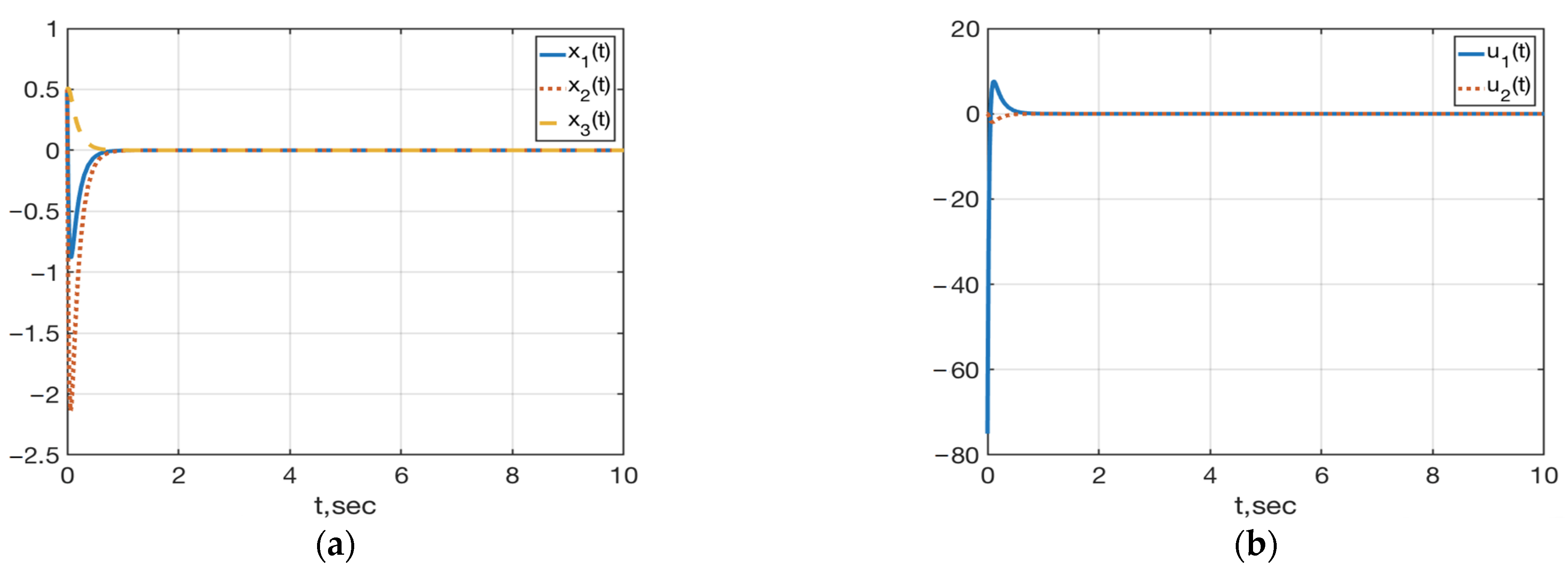
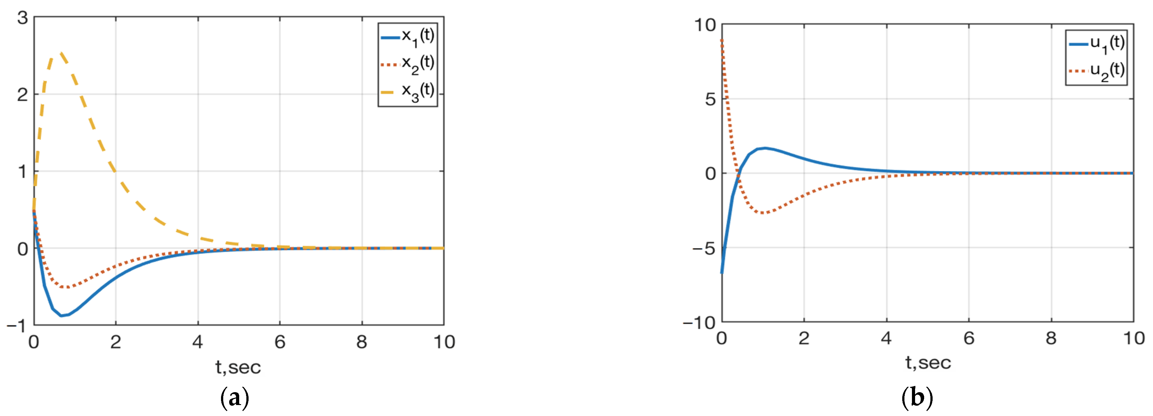
Figure 1 shows the behavior of the variables $x(t)={(x_1(t),\hspace{0.17em}{x}_2(t),\hspace{0.17em}{x}_3(t))}^{\mathrm{T}}$ and controls $u(t)={(u_1(t),\hspace{0.17em}{u}_2(t))}^{\mathrm{T}}$ in closed-loop system (59), (62) with $x(0)={(0.5,\hspace{0.17em}0.5,\hspace{0.17em}0.5\hspace{0.17em})}^{\mathrm{T}}$.

Example 2.

For system (59), the problem is to synthesize a linear feedback that provides a given margin of stability in the closed-loop system $\eta \ge {\eta }_{\mathrm{d}}=1$. To solve this problem, we use the procedure for synthesis of a super-stable closed-loop system (18) based on the transition to the RF (61). We assign the numerical values of the super-stability margin and the elements of the reference matrices of the closed-loop system (18) on the basis of equalities (32) $\nu ={\eta }_{\mathrm{d}}=1,\hspace{0.17em}\hspace{0.17em}{A}_1=-(\nu +\left|a_{11}^{12}\right|+\left|a_{12}^{12}\right|)=-(1+1.25+0.25)=-2.5;\hspace{0.17em}\hspace{0.17em}{a}_1^2=a_2^2=-\nu =-1$, which will ensure that the closed-loop system is super-stable.

$${\dot{e}}_1=-2.5e_1+(1.25\hspace{0.17em}\hspace{0.17em}\hspace{0.17em}-0.25)e_2,\hspace{0.17em}{\dot{e}}_2=\left(\begin{array}{cc}-1& 0\\ 0& -1\end{array}\right)e_2.\hspace{0.17em}\hspace{0.17em}$$

The matrix of this system has a spectrum of $\sigma =\{-1;\hspace{0.17em}-1;\hspace{0.17em}-2,5\}$. This spectrum, and hence a given stability margin, will be provided in the original closed-loop system (59) by the control (19). To determine the local feedback matrix $F_1$, we also use the direct method:

$$A_{11}+A_{10}{F}_1=A_1\Rightarrow 1.5+1.25f_1-0.25f_2=-2.5\iff f_2=16+5f_1.$$

Let us take, for example, $F_1={(-2\hspace{0.17em}\hspace{0.17em}\hspace{0.17em}\hspace{0.17em}6)}^T.$ After performing the transformation (15), we obtain the RF of the closed-loop system (16) in the form

$$\begin{gathered} {\dot{e}}_1=-2.5e_1+(1.25\hspace{0.17em}\hspace{0.17em}\hspace{0.17em}-0.25)e_2,\hspace{0.17em}\hspace{0.17em} \\ {\dot{e}}_2=\left(\begin{array}{l}-7\\ \hspace{0.17em}\hspace{0.17em}18\end{array}\right)e_1+\left(\begin{array}{cc}3.5& -0.5\\ -7& 2\end{array}\right)e_2+\left(\begin{array}{l}2\hspace{0.17em}\hspace{0.17em}\hspace{0.17em}\hspace{0.17em}1\\ 0\hspace{0.17em}\hspace{0.17em}\hspace{0.17em}\hspace{0.17em}1\end{array}\right)u. \end{gathered}$$

The second subsystem of this system gives the control laws for the transformed (17) and initial variables (19) as

$$\begin{gathered} u=\left(\begin{array}{l}0.5\hspace{0.17em}\hspace{0.17em}\hspace{0.17em}-0.5\\ \hspace{0.17em}\hspace{0.17em}0\hspace{0.17em}\hspace{0.17em}\hspace{0.17em}\hspace{0.17em}\hspace{0.17em}\hspace{0.17em}\hspace{0.17em}1\end{array}\right)\left(\left(\begin{array}{l}\hspace{0.17em}\hspace{0.17em}7\\ -18\end{array}\right)e_1+\left(\begin{array}{cc}-3.5& 0.5\\ 7& -2\end{array}\right)e_2+\left(\begin{array}{cc}-1& 0\\ 0& -1\end{array}\right)e_2\right), \\ u=Ke=\left(\begin{array}{ccc}12.5& -5.75& 1.75\\ -18& 7& -3\end{array}\right)e, \\ F=K{T}_{e}T=\left(\begin{array}{ccc}12.5& -5.75& 1.75\\ -18& 7& -3\end{array}\right)\left(\begin{array}{ccc}1& 0& 0\\ 2& 1& 0\\ -6& 0& 1\end{array}\right)\left(\begin{array}{ccc}1& -0.5& 0.5\\ 0& 1& 0\\ 0& 0& 1\end{array}\right), \\ u=Fx=\left(\begin{array}{ccc}-9.5& -1& -3\\ 14& 0& 4\end{array}\right)x. \end{gathered}$$

(63)

The matrix of a closed-loop system (59), (63), expressed as

$$A+BF=\left(\begin{array}{ccc}-8.5& 0& -3\\ -5& -1& -2\\ 15& 0& 5\end{array}\right)$$

is not super-stable, but the system has a given margin of stability:

$$\sigma (A+BF)=\{-1;\hspace{0.17em}-1;\hspace{0.17em}-2,5\},\hspace{0.17em}\min \{-\mathrm{Re}{\lambda }_i(A+BF)\}=1={\eta }_{\mathrm{d}}.$$

Figure 2 shows the behavior of the variables $x(t)={(x_1(t),\hspace{0.17em}{x}_2(t),\hspace{0.17em}{x}_3(t))}^{\mathrm{T}}$ and controls $u(t)={(u_1(t),\hspace{0.17em}{u}_2(t))}^{\mathrm{T}}$ in a closed-loop system (59), (63) with $x(0)={(0.5,\hspace{0.17em}0.5,\hspace{0.17em}0.5\hspace{0.17em})}^{\mathrm{T}}.$

Compared to the system (59), (62) (see Figure 1), the transients of the closed-loop system (59), (63) with real spectrum are not oscillatory but aperiodic, but the range of variation in all the variables has increased by about 2.5 times, and the time of regulation has not significantly changed.

Example 3.

With the nominal system (59) we will consider a parametrically indeterminate system (33), where $\widehat{A}=\alpha A$, $\widehat{B}=\beta B$. Parameters $\alpha ,\hspace{0.17em}\beta$ are constant and unknown, their values belong to closed symmetric intervals with known boundaries:

$$\left|\alpha \right|\le \stackrel{⌢}{\alpha }=0.1, \left|\beta \right|\le \stackrel{⌢}{\beta }=0.1.$$

(64)

The problem is to synthesize a linear feedback that provides a guaranteed margin of stability in a closed-loop system $\eta \ge {\eta }_{\mathrm{d}}=1$ in all uncertainty intervals. In this system,

$$A+\widehat{A}=A(1+\alpha ), B+\widehat{B}=B(1+\beta ), \alpha \ne -1,\hspace{0.17em}\beta \ne -1,$$

(65)

conditions (53), (52) of Lemma 4 are met. The uncertain system is controllable in all uncertainty intervals and keeps the structural controllability properties of the nominal system (59). Hence, the uncertain system is representable in the form of RF (49)–(50) by transformation (12), (51) with matrix (60), where due to (65), ${\widehat{A}}_{ij}=\alpha A_{ij},\hspace{0.17em}i,j=1,\hspace{0.17em}2,\hspace{0.17em}{\widehat{B}}_2=\beta B_2$.

Let us check that the condition (57) is met:

$$\begin{array}{l}{L}_1={\widehat{A}}_{12}{A}_{12}^{+}=\alpha (5/4\hspace{0.17em}\hspace{0.17em}\hspace{0.17em}-1/4)\left(\begin{array}{l}10/13\\ -2/13\end{array}\right)=\alpha =l_{11}^1\hspace{0.17em};\\ L_2={\widehat{B}}_2{B}_2^{-1}=\beta \left(\begin{array}{l}2\hspace{0.17em}\hspace{0.17em}\hspace{0.17em}\hspace{0.17em}1\\ 0\hspace{0.17em}\hspace{0.17em}\hspace{0.17em}\hspace{0.17em}1\end{array}\right)\left(\begin{array}{cc}0.5& -0,5\\ 0& 1\end{array}\right)=\beta I_2,\hspace{0.17em}{l}_{11}^2=l_{22}^2=\beta .\end{array}$$

(66)

Due to (64) $1+\alpha >0,\hspace{0.17em}1+\beta >0,\hspace{0.17em}$ the sufficient condition (57) is fulfilled, and because ${\mu }_1=\hspace{0.17em}{\mu }_2=0.9$, in RF of an uncertain system, it is possible to provide super-stability by means of feedback (55), where

$$S_1=\mathrm{sign}(1+\alpha )=1\hspace{0.17em},\hspace{0.17em}{S}_2=\mathrm{diag}\{\mathrm{sign}(1+\beta )\}=I.$$

In the first subsystem of the uncertain RF ${\dot{x}}_1=(6/4)(1+\alpha )x_1+(5/4\hspace{0.17em}\hspace{0.17em}\hspace{0.17em}-1/4)(1+\alpha )x_2$ let us form the virtual control in the form of (55),

$$x_2=F_1{x}_1=k_1{A}_{12}^{+}{S}_1{x}_1=k_1\left(\begin{array}{l}10/13\\ -2/13\end{array}\right)x_1.$$

(67)

With variable changes $e_1:=x_1,\hspace{0.17em}{e}_2=x_2-F_1{x}_1$ we obtain

$${\dot{e}}_1=(1+\alpha )((A_{11}+k_1)e_1+A_{12}{e}_2)=(1+\alpha )((1.5+k_1)e_1+(1.25\hspace{0.17em}\hspace{0.17em}\hspace{0.17em}\hspace{0.17em}\hspace{0.17em}-0.25)e_2).$$

As can be seen, in this subsystem the choice of gain $k_1$ does not depend on undefined parameters. Let us assume $\nu ={\eta }_{\mathrm{d}}=1$; then, similarly to (21), we have

$$-(1.5+k_1)-(1.25+0.25)\ge 1\Rightarrow k_1\le -4.$$

For the convenience of the calculation (67), let us assume $k_1=-13/2=-6.5$, then $F_1={(-5\hspace{0.17em}\hspace{0.17em}\hspace{0.17em}\hspace{0.17em}\hspace{0.17em}1)}^T$. Let us perform transformations (15) taking into account (61), (65)–(67), forming the control law in the form (55), that is,

$$u=K_2{e}_2=k_2{B}_2^{-1}{S}_2{e}_2=k_2\left(\begin{array}{cc}0.5& -0,5\\ 0& 1\end{array}\right)e_2,$$

(68)

and we obtain a closed RF of the uncertain system in terms of discrepancies in the form (56), namely,

$$\begin{array}{l}{\dot{e}}_1=(1+\alpha )(-5e_1+(1.25\hspace{0.17em}\hspace{0.17em}\hspace{0.17em}\hspace{0.17em}-0.25)e_2,\\ {\dot{e}}_2=(1+\alpha )\left(\begin{array}{l}-30\\ \hspace{0.17em}\hspace{0.17em}3\end{array}\right)e_1+\left((1+\alpha )\left(\begin{array}{cc}7.25& -1.25\\ -0.75& 0.75\end{array}\right)+k_2(1+\beta )\left(\begin{array}{cc}1& 0\\ 0& 1\end{array}\right)\right)e_2.\end{array}$$

From the second inequality (58), we find the second gain

$$\begin{gathered} {\overline{k}}_{21}\le -(1+(1+\stackrel{⌢}{\alpha })(30+7.25+1.25))/(1-\stackrel{⌢}{\beta })\approx -48.2, \\ {\overline{k}}_{22}\le -(1+(1+\stackrel{⌢}{\alpha })(3+0.75+0.75))/(1-\stackrel{⌢}{\beta })\approx -6.62,k_2\le \min \{-48.2;\hspace{0.17em}\hspace{0.17em}-6.62\}. \end{gathered}$$

Let us take $k_2=-50$. Then due to (68), (19), we get

$$\begin{gathered} u=Ke,\hspace{0.17em}\hspace{0.17em}K=(O\hspace{0.17em}\hspace{0.17em}\hspace{0.17em}\hspace{0.17em}\hspace{0.17em}\hspace{0.17em}{K}_2)=\left(\begin{array}{ccc}0& -25& 25\\ 0& 0& -50\end{array}\right), \\ F=K{T}_{e}T=\left(\begin{array}{ccc}0& -25& 25\\ 0& 0& -50\end{array}\right)\left(\begin{array}{ccc}1& 0& 0\\ 5& 1& 0\\ -1& 0& 1\end{array}\right)\left(\begin{array}{ccc}1& -0.5& 0.5\\ 0& 1& 0\\ 0& 0& 1\end{array}\right). \end{gathered}$$

Control law

$$u=Fx=\left(\begin{array}{ccc}-150& 50& -50\\ 50& -25& -25\end{array}\right)x$$

(69)

provides in the initial uncertain system a guaranteed margin of stability $\eta \ge \nu ={\eta }_{\mathrm{d}}=1$ in all uncertainty intervals, and this solves the problem. For example, in the nominal system (59) and in the uncertain system with different boundary values of parameters $\alpha =\pm 0.1,\hspace{0.17em}\beta =\pm 0,1$ we obtain

$$\begin{gathered} \sigma (A+BF)=\{-6.0531;\hspace{0.17em}-41.5559;\hspace{0.17em}-49.3910\},\eta =6.0531; \\ \sigma (1.1A+0.9BF)=\{-7.0628;\hspace{0.17em}-35.3071;\hspace{0.17em}-44.33\},\hspace{0.17em}\eta =7.0628; \\ \sigma (1.1A+1.1BF)=\{-6.6585;\hspace{0.17em}-45.7114;\hspace{0.17em}-54.3301\},\hspace{0.17em}\eta =6.6585; \\ \sigma (0.9A+1.1BF)=\{-5.2231;\hspace{0.17em}-47.625;\hspace{0.17em}-54.4519\},\hspace{0.17em}\eta =5.2231; \\ \sigma (0.9A+0.9BF)=\{-5.4478;\hspace{0.17em}-37.4003;\hspace{0.17em}-44.4519\},\hspace{0.17em}\eta =5.4478. \end{gathered}$$

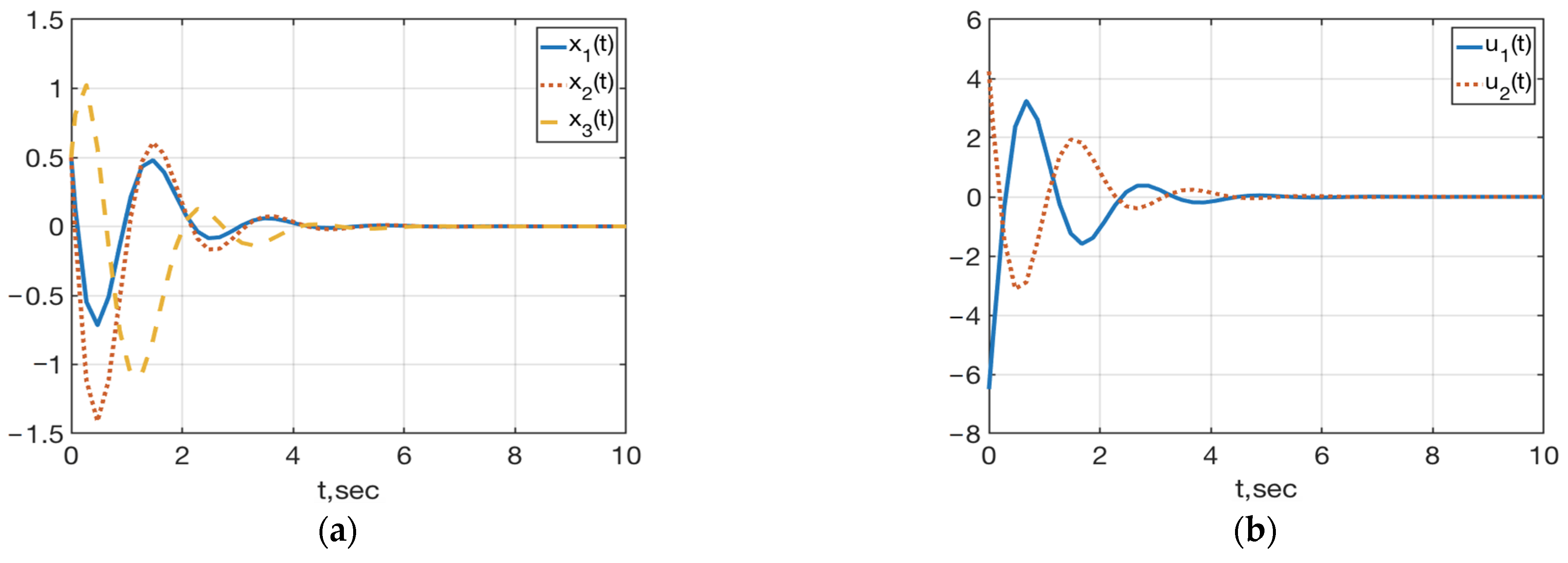
Figure 3 shows the behavior of the state variables $x(t)={(x_1(t),\hspace{0.17em}{x}_2(t),\hspace{0.17em}{x}_3(t))}^{\mathrm{T}}$ and controls $u(t)={(u_1(t),\hspace{0.17em}{u}_2(t))}^{\mathrm{T}}$ in the closed-loop system $\dot{x}=(1.1A+0.9BF)x$, (59), (69) with $x(0)={(0.5,\hspace{0.17em}0.5,\hspace{0.17em}0.5\hspace{0.17em})}^{\mathrm{T}}$.

In comparison with system (59), (63) (see Figure 2), the solution norm of the closed-loop system is practically the same, but the regulation time has been reduced by about 6 times. In addition, the value of $\Vert u(0)\Vert$ has increased by about 10 times.

It should be noted that the control spikes at the beginning of the transient can be limited by piecewise linear control with saturation

$$\overline{u}={(10\mathrm{sat}(u_1),\hspace{0.17em}10\mathrm{sat}(u_2))}^{\mathrm{T}}.$$

(70)

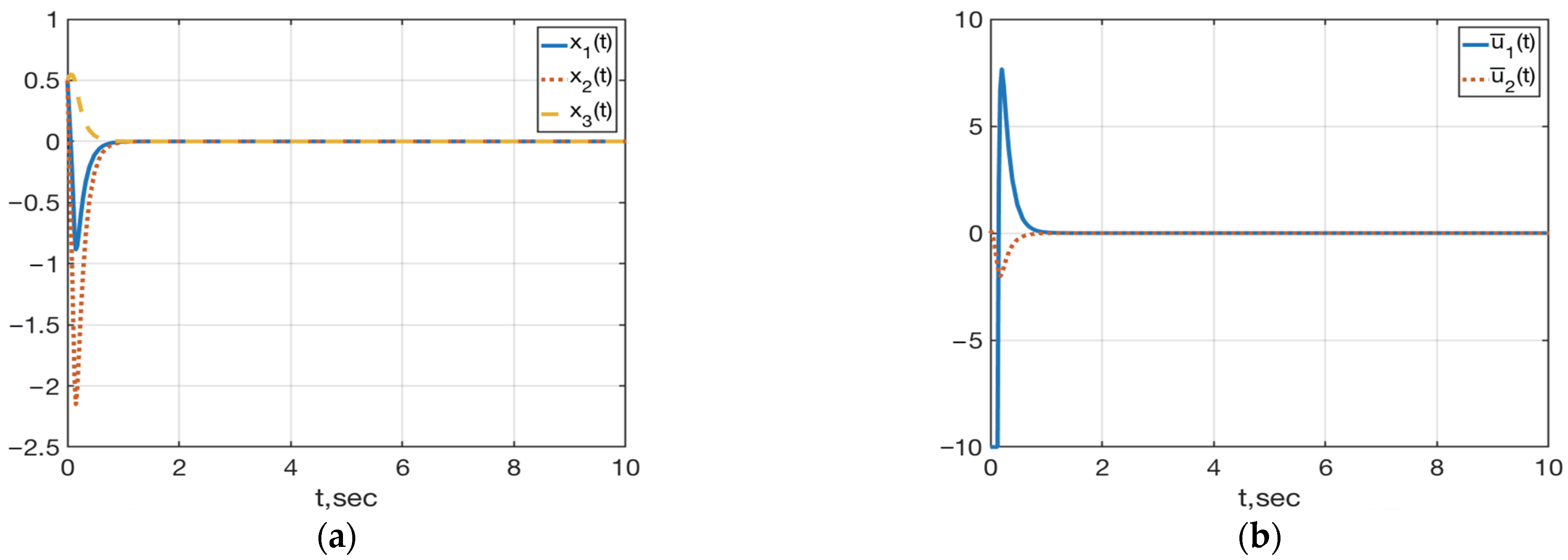
Corresponding graphs for the closed-loop system $\dot{x}=(1.1A+0.9BF)x$, (59), (69), (70) are shown in Figure 4. As can be seen from Figure 3a and Figure 4a, the control constraint (70) had no effect on the state variable transients.

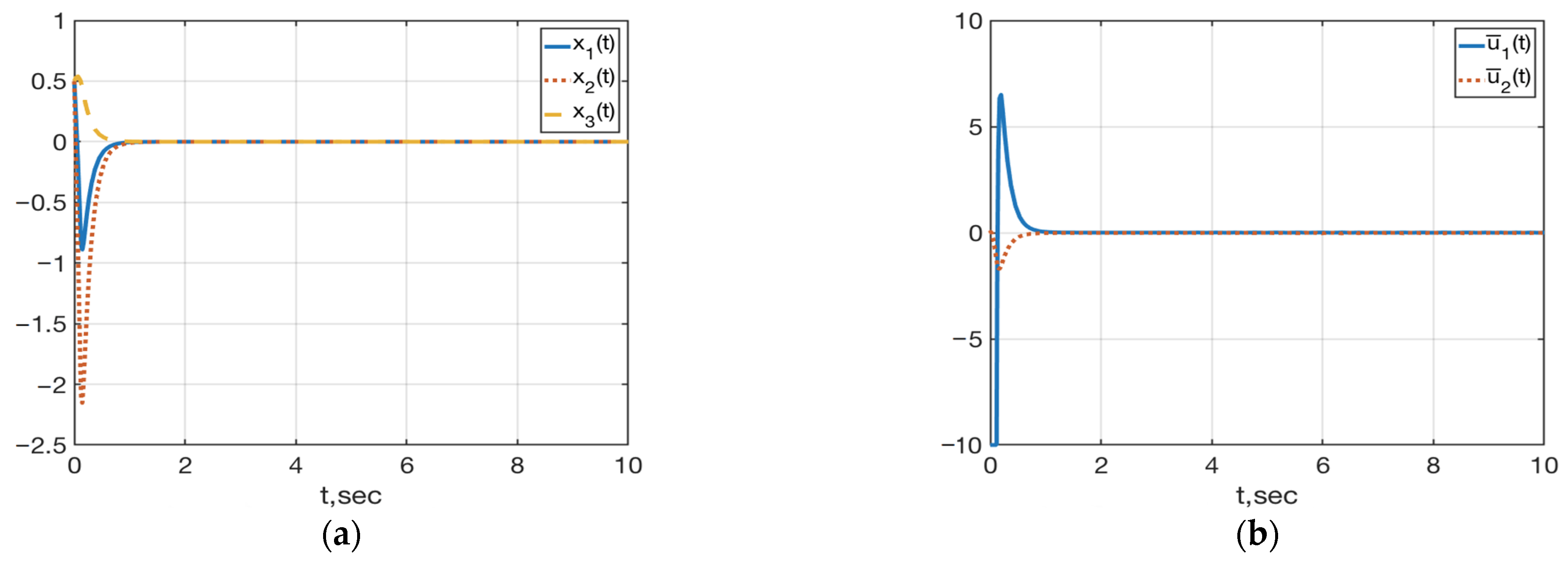
Figure 5 shows the behavior of the variables $x(t)={(x_1(t),\hspace{0.17em}{x}_2(t),\hspace{0.17em}{x}_3(t))}^{\mathrm{T}}$ and control vector $u(t)={({\overline{u}}_1(t),\hspace{0.17em}{\overline{u}}_2(t))}^{\mathrm{T}}$ in a closed-loop system $\dot{x}=((1+\alpha )A+(1+\beta )BF)x$, (59), (69), (70), $x(0)={(0.5,\hspace{0.17em}0.5,\hspace{0.17em}0.5\hspace{0.17em})}^T$, where the unknown parameters smoothly vary within the specified ranges (64): $\alpha =0.1\sin 4t,\hspace{0.17em}\beta =0.1\sin 2t$. As we can see, at variable parameters the nature of the transients is practically unchanged, a fact that opens perspectives for using the developed approach in relation to parametrically uncertain non-stationary control systems.

5. Discussion

In this paper, we propose a new approach to the synthesis of robust control for a practically significant class of linear stationary parametrically uncertain systems, in which the structural controllability properties of the nominal system do not change with parameter variation within acceptable limits. For the special case of systems with a controllability indicator equal to two, the procedures for the synthesis of a stabilizing feedback are formalized in detail, using the concepts of regular form and super-stability. The possibility of extending this approach to a general form of controllable systems is shown theoretically.

It should be noted that the tuning of the feedback coefficients, which guarantee a given margin of stability in the closed-loop system in all uncertainty intervals, is done on the basis of inequalities in terms of matrix elements rather than their eigenvalues. On the one hand, this is what allows synthesizing of a robust system. However, on the other hand, these conditions are only sufficient, and the resulting estimates are conservative. As a result, there may be spikes in the start of transients of state variables and controls that are not acceptable in practical applications.

Numerical examples show the fundamental possibility of limiting the control actions, as well as the performance of the proposed method for non-stationary systems. However, further research is needed to formalize these problems rigorously.

References

1. Utkin, V.A.; Utkin, A.V. Problem of Tracking in Linear Systems with Parametric Uncertainties under Unstable Zero Dynamics. Autom. Remote Control 2014, 75, 1577–1592. [Google Scholar] [CrossRef]
2. Ljung, L. Pespectives on system identification. IFAC Annu. Rev. 2010, 34, 1–12. [Google Scholar] [CrossRef] [Green Version]
3. Krstic, M.; Kanellakopoulos, I.; Kokotovic, P. Nonlinear and Adaptive Control Design; Wiley: New York, NY, USA, 1995. [Google Scholar]
4. Ackermann, J. Robust Control: The Parameter Space Approach; Springer: London, UK, 2002. [Google Scholar]
5. Kharitonov, V.L. Asymptotic Stability of a Family of Systems of Linear Differential Equations. Differ. Uravn. 1978, 1, 2086–2088. [Google Scholar]
6. Lao, X.X. Necessary and sufficient conditions for stability of a class of interval matrices. Int. J. Control 1987, 45, 211–214. [Google Scholar]
7. Polyak, B.T.; Tsypkin, Y.Z. Frequency Criteria of Robust Stability and Aperiodicity of Linear Systems. Autom. Remote Control 1990, 9, 1192–1200. [Google Scholar]
8. Neimark, Y.I. Robust stability and D-partitioning. Autom. Remote Control 1992, 53, 957–965. [Google Scholar]
9. Gadewadikar, J.; Lewis, F.L.; Abu-Khalaf, M. Necessary and Sufficient Conditions for H-infinity Static Output-Feedback Control. J. Guid. Control Dyn. 2006, 29, 4. [Google Scholar] [CrossRef] [Green Version]
10. Edwards, C.; Shtessel, Y.B. Adaptive Continuous Higher Order Sliding Mode Control. Automatica 2016, 65, 183–190. [Google Scholar] [CrossRef] [Green Version]
11. Antipov, A.S.; Krasnova, S.A.; Utkin, V.A. Methods of Ensuring Invariance with Respect to External Disturbances: Overview and New Advances. Mathematics 2021, 9, 3140. [Google Scholar] [CrossRef]
12. Polyak, B.T.; Sznaider, M.; Shcherbakov, P.S.; Halpern, M. Super-stable control systems. In Proceedings of the 15th IFAC, Barcelona, Spain, 21–26 July 2002; pp. 799–805. [Google Scholar]
13. Utkin, V.I.; Yang, K.D. Methods for construction of discontinuity planes in multidimensional variable structure systems. Autom. Remote Control 1979, 39, 1466–1470. [Google Scholar]
14. Drakunov, S.V.; Izosimov, D.B.; Luk’yanov, A.G.; Utkin, V.A.; Utkin, V.I. The Block Control Principle. Autom. Remote Control 1990, 5, 601–608. [Google Scholar]
15. Krasnova, S.A.; Utkin, V.A.; Utkin, A.V. Block approach to analysis and design of the invariant nonlinear tracking systems. Autom. Remote Control 2017, 78, 2120–2140. [Google Scholar] [CrossRef]
16. Krasnova, S.A.; Utkin, V.A.; Sirotina, T.G. A structural approach to robust control. Autom. Remote Control 2011, 72, 1639–1666. [Google Scholar] [CrossRef]
17. Gantmacher, F.R. Theory of Matrices; Chelsea Publishing Company, Inc.: New York, NY, USA, 1959. [Google Scholar]
18. Mu, J.; Yan, X.-G.; Spurgeon, S.K.; Mao, Z. Generalized regular form based smc for nonlinear systems with application to a wmr. IEEE Trans. Ind. Electron. 2017, 64, 6714–6723. [Google Scholar] [CrossRef] [Green Version]
19. Wonham, W.F. Linear Multivariate Control: A Geometric Approach; Springer: New York, NY, USA, 1985. [Google Scholar]
Figure 1. (a) Plots of x 1 ( t ) , x 2 ( t ) , x 3 ( t ) ; (b) Plots of u 1 ( t ) , u 2 ( t ) in the closed-loop system (59), (62) with x ( 0 ) = ( 0.5 , 0.5 , 0.5 ) T .
Mathematics 10 00098 g001
Figure 2. (a) Plots of x 1 ( t ) , x 2 ( t ) , x 3 ( t ) ; (b) Plots of u 1 ( t ) , u 2 ( t ) in the closed-loop system (59), (63) with x ( 0 ) = ( 0.5 , 0.5 , 0.5 ) T .
Mathematics 10 00098 g002
Figure 3. (a) Plots of x 1 ( t ) , x 2 ( t ) , x 3 ( t ) ; (b) Plots of u 1 ( t ) , u 2 ( t ) in the closed-loop system x ˙ = ( 1.1 A + 0.9 B F ) x , (59), (69) with x ( 0 ) = ( 0.5 , 0.5 , 0.5 ) T .
Mathematics 10 00098 g003
Figure 4. (a) Plots of x 1 ( t ) , x 2 ( t ) , x 3 ( t ) ; (b) Plots of u ¯ 1 ( t ) , u ¯ 2 ( t ) in the closed-loop system x ˙ = ( 1.1 A + 0.9 B F ) x , (59), (69), (70).
Mathematics 10 00098 g004
Figure 5. (a) Plots of x 1 ( t ) , x 2 ( t ) , x 3 ( t ) ; (b) Plots of u ¯ 1 ( t ) , u ¯ 2 ( t ) in the closed-loop system x ˙ = ( ( 1 + α ) A + ( 1 + β ) B F ) x , (59), (69), (70), x ( 0 ) = ( 0.5 , 0.5 , 0.5 ) T .
Mathematics 10 00098 g005
Publisher’s Note: MDPI stays neutral with regard to jurisdictional claims in published maps and institutional affiliations.