Improving Calculus Curriculum in Engineering Degrees: Implementation of Technological Applications

Abstract

The teaching of mathematics has always concerned all the professionals involved in engineering degrees. Curently students have less interest in these studies, what has caused an increase of this concern. The lack of awareness of students about the significance of mathematics in their careers, provoke the decrease of undergraduate students’ motivation, which derives in a low interest in engineering degrees. The aim of this work is that engineering students achieve a greater motivation and involvement in first academic courses, through the implementation of real and technological applications related to their degrees in the learning of mathematical concepts. To this end, the 2019/2020 and 2020/2021 academics years, the seminar “Applications of Multivariable Calculus in Engineering” has been held in Universitat Politècnica de Catalunya-BarcelonaTech (UPC), based on the teaching of Multivariable Calculus by the execution of real problems where calculus concepts are necessary to solve them. With the aim of analyzing students’ motivation and assessment of the seminar, anonymous surveys and personal interviews have been conducted. The number of attending students to the sessions in each academic year has been 16 and all of them have been participants in the surveys and interviews. The results show that students’ responses were generally positive and they agree that their motivation to the subject Multivariable Calculus has increased with the use of real applications of mathematics. The execution of practical problems with engineering applications improves the acquirement of mathematical concepts, what could imply an increase of students’ performance and a decrease of the dropout in the first academic courses of engineering degrees.

1. Introduction

The economic development of countries is mainly based on technology. Thus, professionals in fields related to science, technology, engineering and mathematics (STEM) are necessary to improve the economy of countries. Technological production implies encouraging and supporting students to become technological professionals. Therefore, STEM disciplines are considered essential for the economic development of technological societies. The potential negative economic impact of undersupply is of concern due to opportunity costs and loss of competitiveness [1]. In addition, STEM education could integrate students’ skills and better professional competences. The 21st century, as the age of information technologies, entails new job prospects and upcoming jobs which require new skills from professionals. Nowadays, technology is necessary in many jobs such as science, business, engineering, etc.

Moreover, high occupancy demands for STEM degrees are expected [2,3]. As technological knowledge and expertise is becoming more specialized and economically increasingly important, ever more jobs specialized in STEM disciplines are required and this demand is expected to further increase in the upcoming years, as remarked in [4,5].

However, at the present time in most countries, undergraduate students have less interest in technological degrees [1,6,7], which is mainly due to the lack of awareness of the importance of mathematical subjects in first academic courses of these studies. This lack of awareness derives, in most cases, in the decrease of students’ motivation, which has as a result a low performance and a high dropout rate in the first years of these degrees. Thus, the engineering education community work to identify the causes of this situation, as indicates [2].

The worrying dropout in higher education has gained much interest in academic research. One third of undergraduate students leave university without obtaining a degree, mainly during their first academic year [8]. The dropout rate is higher in STEM careers [7].

The importance of students’ motivation and engagement has been analyzed in previous studies [9,10], and in particular for technological degrees [11]. In first academic years is essential to promote student engagement [12,13], which involves the improvement of motivation [14,15], relatedness [16], student achievement [17] and academic performance [18], what imply the decrease of the dropout rate.

Practical and real applications used in mathematics subjects of engineering degrees, encourage student engagement and motivation [14], as has been studied in previous works [19,20,21,22,23]. A proper coordination among mathematical subjects and technological subjects of engineering degrees syllabus contribute to the decrease of dropout rates [24]. Active learning has positive results on the rise of students’ motivation and on the enhancement of their learning, what entails the improvement of their performance, as it is stated in several studies [25,26,27,28]. For instance, the relationship between mathematical creativity and the relevance of problem-solving in the teaching of mathematics has been studied in [29]. Moreover, key employee expected abilities involve problem-solving and analytical thinking skills besides the competences to communicate them. The use of problem-posing in engineering degrees contributes to increase student involvement. This methodology consists of exposing a problem to students, related to technological disciplines, which will lead them to discover what they need to learn to solve this problem. Furthermore, it implies the development of essential abilities and competences for their career, as they are autonomy, continuous learning, critical thinking, planning and communications skills [30,31]. Moreover, the integration of theory and practice entails the improvement of motivation, what implies an increase of academic performance [32,33,34,35].

The purpose of this work is to generate an integrated STEM curricula, connecting mathematical applications with STEM education. The aim of the present study is to increase undergraduate engineering students’ motivation by contextualization of mathematical subjects with technological applications related to the disciplines taught in the following academic courses of these degrees. The material developed in this work is expected to be introduced for a future adaptation of mathematical subjects’ syllabus in engineering degrees.

Engineering students have to solve engineering problems and mathematical methodologies are the tools to solve them. They need to know the usefulness of mathematics and how essential they are for their degrees and their future careers. In this regard, the motivation and involvement of students are considered a key element, clarifying the importance of mathematics for technological subjects and for their future profession.

This study is part of the work “Applications of Mathematics in Engineering”, which is formed by two seminars: “Applications of Linear Algebra in Engineering” [36] and “Applications of Multivariable Calculus in Engineering”. These two seminars entail the mathematical subjects of first academic courses in technological degrees. This study focuses on the seminar “Applications of Multivariable Calculus in Engineering”, whose purpose is to present real and technical applications of Multivariable Calculus related to engineering degrees with the objective of increasing students’ motivation towards the learning of mathematics in first academic courses. Knowing the need of mathematical concepts to solve those technical applications, students realized of the importance of mathematics not only for the execution of their degrees but also for the development of their careers as engineers.

This article focuses on these research questions:

• How does the implementation of real and practical applications in mathematical subjects’ influence on students’ motivation?
• What are the benefits of including real and practical applications in mathematical subjects of first academic courses in technological degrees?

The results of the study show that for students is really motivating to know what they will be capable to do in the next courses of their degree. They also realized of how essential Multivariable Calculus is for their future profession and increased their interest towards the subject.

These results verifies that this experience lets students obtain a greater understanding of mathematical concepts, which increases students’ performance in mathematical subjects of engineering degrees.

2. Materials and Methods

The study has been conducted at the Universitat Politècnica de Catalunya-BarcelonaTech (UPC), a public university specialised in STEM degrees. The work “Applications of Mathematics in Engineering” is formed by two seminars: “Applications of Linear Algebra in Engineering” [36] and “Applications of Multivariable Calculus in Engineering”, which started in the 2019/2020 academic year and were undertaken in the first and the second semester, respectively. Both seminars were organised in weekly sessions of one hour and a half each session. These sessions have been held also in the 2020/2021 academic year and it is planned to repeat them during the following years.

Thus, since the 2019/2020 academic year, weekly sessions have been given to first-year students of the Industrial Engineering Bachelor’s Degree from the Barcelona School of Industrial Engineering (ETSEIB) of the UPC, this degree lasts four years. Currently, the syllabus of mathematical subjects in engineering degrees do not content technological applications. Mathematical subjects focus on mathematical concepts, they are not contextualized in the technological disciplines of engineering degrees. The aim of this work is to contextualize mathematics through the connection of mathematical subjects with technological disciplines, taught in the following academic courses, and with their future technological professions. Thus, students will be able to realize of the importance of mathematics for engineering, as well as they learn engineering applications from the beginning of their degrees.

The two seminars “Applications of Linear Algebra in Engineering” and “Applications of Multivariable Calculus in Engineering” are offered in the same semesters in which the ordinary classes of the compulsory subjects Linear Algebra and Multivariable Calculus are taught, first and second semesters, respectively, so that the students who wish could complement in a parallel way and from a practical point of view the theoretical concepts introduced in the ordinary classes. The seminars have been devised with the aim of increasing students’ motivation and involvement in the early stages of engineering studies. In addition to the benefits of these sessions, Universitat Politècnica de Catalunya-BarcelonaTech (UPC) recognizes with 1 European Credit Transfer and Accumulation System (ETCS) the attendance for students.

This article focuses on the seminar “Applications of Multivariable Calculus in Engineering”. In each of the sessions of this seminar, applications illustrating the use of mathematical concepts related to multivariable calculus in different engineering areas are explained. The compulsory subject of Multivariable Calculus lasts one semester (14 weeks). Instead, the optional seminar presented in this work consists of 10 weeks. During the first two weeks of the semester, students are informed of the existence of this seminar in order to enable registration; and two other weeks, before the partial and final exams, no seminar sessions are given. So, this seminar consists of 10 sessions, 8 main sessions and 2 review sessions. The 8 main sessions are detailed in

Table 1. Applications of Multivariable Calculus in Engineering.

Session	Title
1	“Discontinuous phenomena: hysteresis, caustics”
2	“Thom’s catastrophes”
3	“Taylor and Fourier series”
4	“Chain, implicit and inverse theorems”
5	“Inverse kinetics”
6	“Kinematics of mechanisms with links”
7	“Optimization”
8	“Miscellany”

.

To evaluate the results of this study, anonymous surveys and personal interviews were conducted, with the aim of analyzing students’ appreciation of the seminar “Applications of Multivariable Calculus in Engineering”.

Surveys were undertaken at the end of each session and evaluate the impact of the experience on the students attending to the sessions, as regards the mathematical and engineering contents, the technological applications and the motivation towards the subject of Multivariable Calculus. These surveys consisted of five questions which must be valued on a 5-point scale (1 = Strongly disagree, 2 = Disagree, 3 = Nor agree nor disagree, 4 = Agree, 5 = Strongly agree). In addition, there is the possibility to include an opinion, where students could explain their impression about the session. The questions set in the surveys were:

Question 1: The assessment of mathematical contents is positive.

Question 2: The assessment of engineering contents is positive.

Question 3: The sessions “Applications of Multivariable Calculus in Engineering” let students know technological applications of different mathematical concepts.

Question 4: The applications of mathematical concepts achieve to increase the motivation to the subject Multivariable Calculus.

Question 5: The execution of practical exercises with technological applications improve the learning of mathematical concepts.

With the aim of extracting more opinions from the students attending the sessions “Applications of Multivariable Calculus in Engineering”, personal interviews have been undertaken at the end of all the sessions in 2019/2020 and 2020/2021 academic years, which consisted of several open questions, where students could express in detail their opinion and assessment of the sessions. It should be noted that, in order to avoid bias in the answers, the person who interviewed students was not a professor but a master’s student. The main questions set to students were:

• What aspects do you assess most positively of these sessions?
• What applications have been more interesting? Why?
• How have these sessions influenced on your motivation and on your interest toward Multivariable Calculus?
• Have these sessions helped you understand mathematical concepts of the subject Multivariable Calculus? What applications? What concepts?
• After these sessions, do you consider that Mathematics are more important and essential to the development of engineering degrees? How? Why?

The influence of the implementation of the seminar “Applications of Multivariable Calculus in Engineering” on the students attending the seminar has been analyzed from the answers to the surveys and to the interviews undertaken after the sessions of this seminar.

3. Results

3.1. Students’ Mathematical Contents

The 8 main sessions of the seminar “Applications of Multivariable Calculus in Engineering” consists of real and practical applications of the contents developed in the subject Multivariable Calculus, whose syllabus is:

• Continuity and derivability of multivariable functions.
• Integration of multivariable functions.
• Laplace transform and Fourier series.

The first three sessions of the seminar are focused in discontinuous phenomena. Although they are not still included in mathematical subject programmes, discontinuous phenomena are very common in engineering problems and entail most of the contents of engineering subjects and contribute to illustrate the importance of these mathematical theories to solve real engineering problems. The applications developed in sessions 1, 2 and 3 include the Thom’s catastrophes and Taylor and Fourier series.

The sessions 4, 5 and 6 are related to differential calculus and the basic theorems: chain rule, implicit function theorem and inverse function theorem, which are the basis of a great number of classical applications in engineering.

The session 7 is about optimization, which is the most important goal of engineering.

The last session, miscellany, deal with the use of engineering vision to solve applications in order to apply mathematical calculations, concluding that engineers must complement the use of mathematical tools with their engineering knowledge.

Some practical and real applications explained to the students in the sessions “Applications of Multivariable Calculus in Engineering” are explained below. They consist of applications of Multivariable Calculus related to engineering disciplines which can be understood and learnt by undergraduate students in the first academic courses.

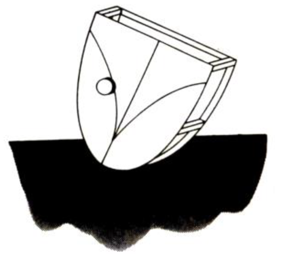
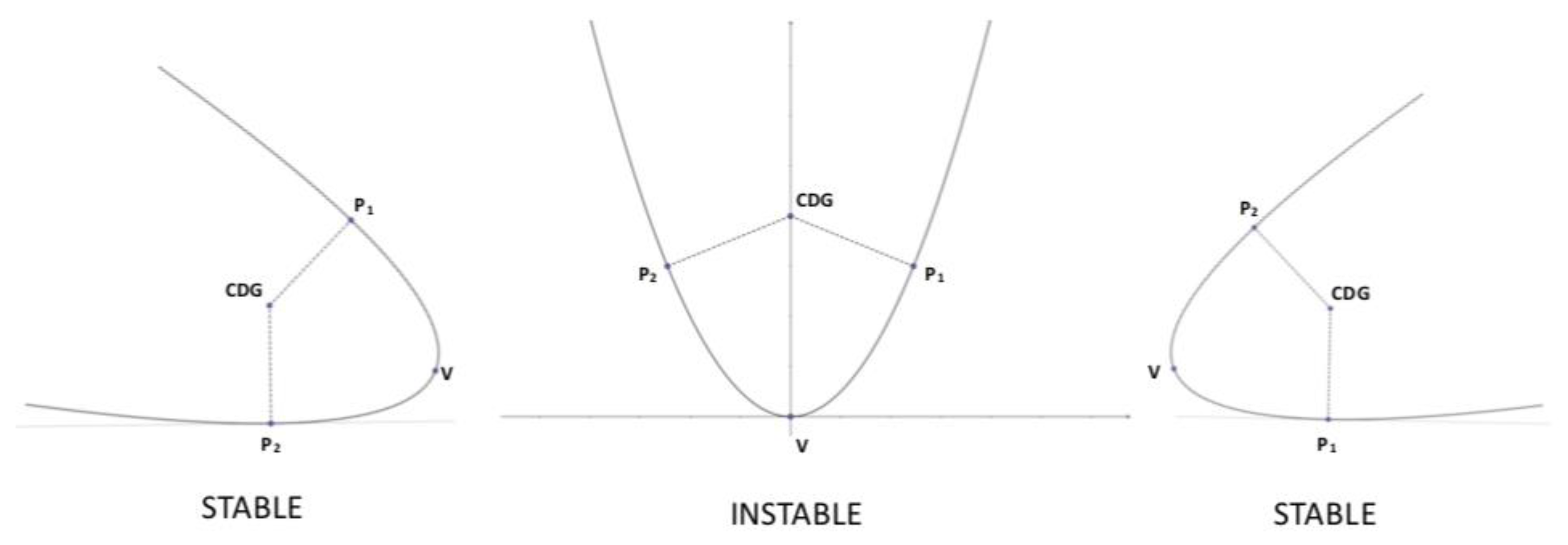
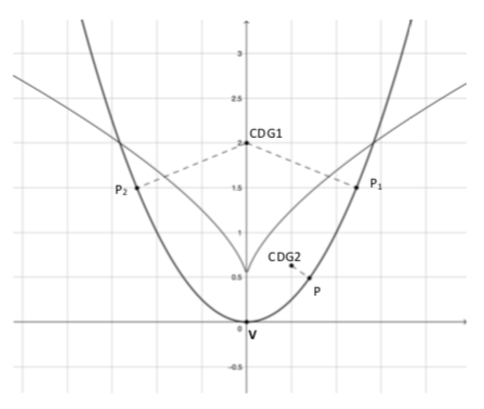
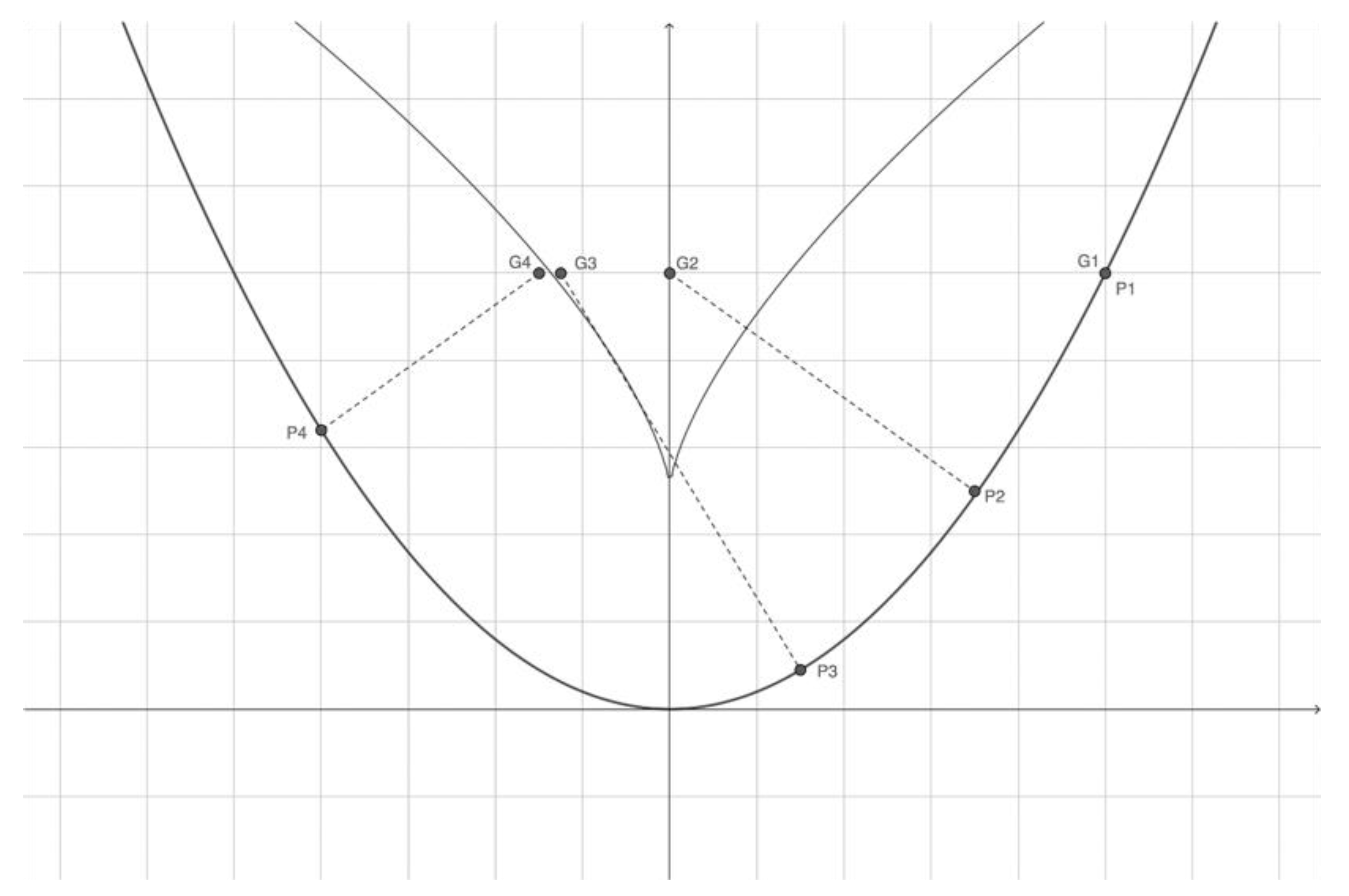
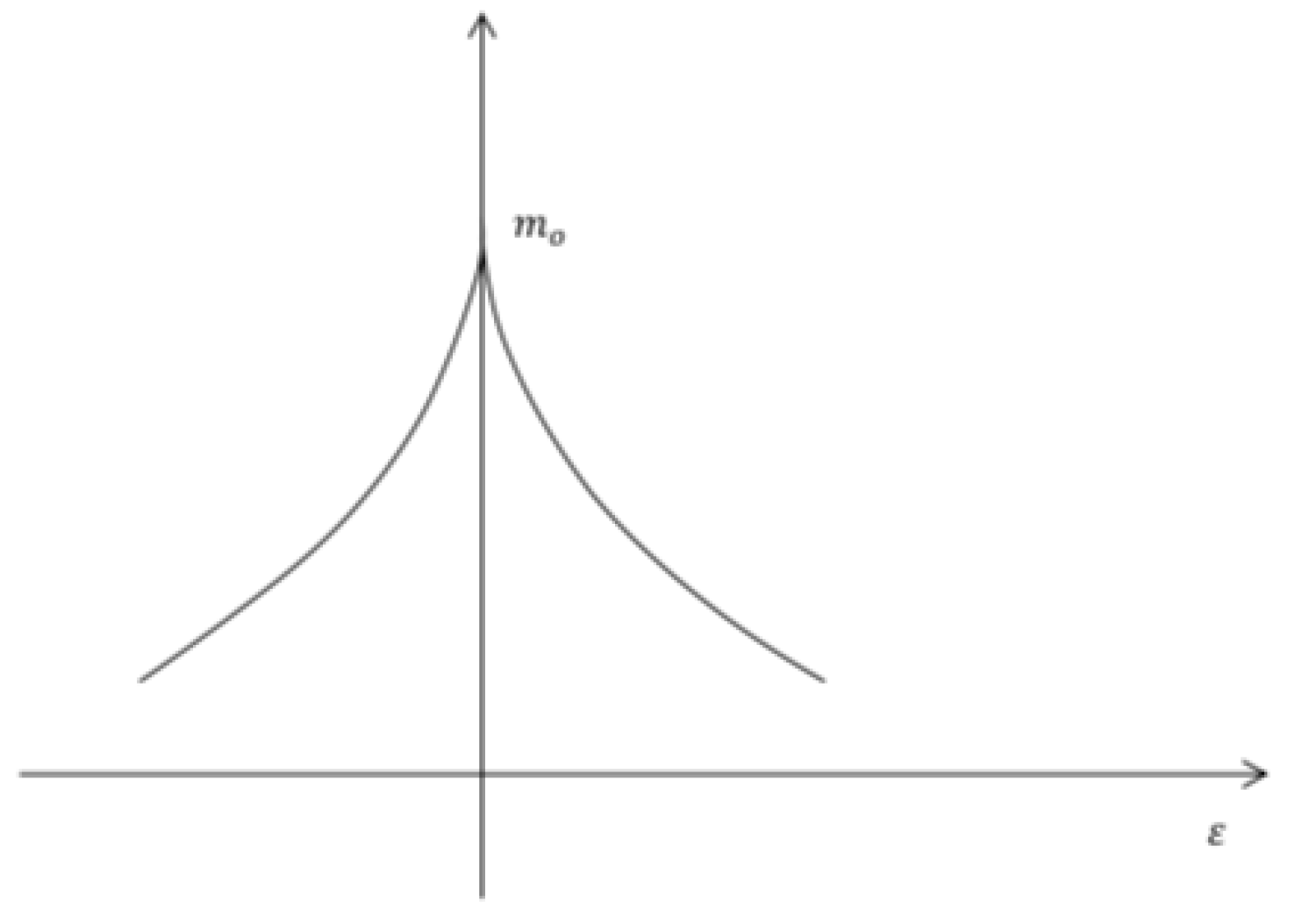
3.1.1. Application 1: A Gravitational Machine

The first application is an example of discontinuous phenomena and it was explained in the session 1 (Discontinuous phenomena: hysteresis, caustics), where discontinuous phenomena were introduced highlighting how frequent they are in engineering.

In a gravitational machine appear discontinuous phenomena as it is going to be shown hereunder. A gravitational machine consists of a flat sheet limited by a parabola, leant on a horizontal plane. The most important point of this machine is that the center of gravity (CDG) is variable through the position of a magnet which can be moved on the sheet surface. Supposing the sheet mass negligible, the CDG would be the magnet position (Figure 1).

When the CDG is displaced on the sheet, how will the sheet situate in a stable way?

The stability situation will happen when the CDG is placed in a minimum height, therefore the stable equilibrium point P on the parabola outline is the relative minimum of the distance between the CDG and the parabola points, that is, the orthogonal base to the parabola from the CDG, as it is shown in the following figure (Figure 2).

If CDG is placed on the parabola vertical axis, the equilibrium point could be stable or instable depending on the CDG height. If the distance between the CDG and the equilibrium point is a relative minimum, there would be stable equilibrium but if this distance is a relative maximum, the equilibrium point is the parabola vertex and it would be instable equilibrium.

If we consider the parabola $\left\{\left(z,z^2\right),\left|z\right|\le 2\right\}$ and the CDG $=\left(0,2\right)$, the distance between any point on the parabola outline and the CDG placed on the parabola axis would be:

$$E={\left(d\left(z,z^2\right),\left(0,2\right))\right)}^2=z^2+{\left(z^2-2\right)}^2=z^4-3z+4$$

(1)

If we derivate and equal to zero, we obtain:

$$D{\left(d\left(\left(z,z^2\right),\left(0,2\right)\right)\right)}^2=4z^3-6z=0$$

(2)

where $z=0$ is a relative maximum and $z=\pm \sqrt{\raisebox{1ex}{$3$}\!\left/ \!\raisebox{-1ex}{$2$}\right.}$ are relative minimums.

Therefore, if CDG is = (0,2), there is instable equilibrium in the parabola vertex, $V=\left(0,0\right)$. In addition, there is stable equilibrium on the parabola outline points $P_1=\left(\sqrt{\frac{3}{2}},\frac{3}{2}\right)$, $P_2=\left(-\sqrt{\frac{3}{2}},\frac{3}{2}\right)$. These points are indicated in the following figure (Figure 3):

If the CDG height is less than $\raisebox{1ex}{$1$}\!\left/ \!\raisebox{-1ex}{$2$}\right.$. there is only one relative extreme, which is the parabola vertex and, in this case, there would be 1 stable equilibrium point.

Depending on the position of de CDG, there can exist three equilibrium points or only one equilibrium point. This situation happens not only if the CDG is placed on the parabola axis but also on any point inside the parabola.

The question is in what positions of the CDG, there are three equilibrium points (two stable points and one instable point) and in what positions there is only one stable equilibrium point. To answer this question, we must analyze in what positions of the CDG there are three orthogonals, corresponding to two relative minims and one relative maxim and in what positions there is only one equilibrium point, corresponding to a relative minim. To solve it we have to make the orthogonals envelope. We must distinguish the area where there are three orthogonals and the area with only one orthogonal, the separation between these two areas is the orthogonals envelope. To obtain the expression of this envelope, we have to do the following calculations.

The orthogonal in:

$$\left(z,z^2\right)=\left\{\left(\beta ,\alpha \right):\frac{\beta -z}{-2z}=\alpha -z^2\right\}$$

(3)

The expression of the orthogonal is:

$$0=\beta -z+2z\left(\alpha -z^2\right)=\beta +\left(2\alpha -1\right)z-2z^3$$

(4)

To eliminate z, we calculate the derivative:

$$0=D^Z(\beta -z+2z\left(\alpha -z^2\right))=\left(2\alpha -1\right)-6z^2$$

(5)

with these 2 expressions, we can obtain that:

$$\begin{gathered} z^2=\frac{2\alpha -1}{6}\Rightarrow 0=\beta +z\left(\left(2\alpha -1\right)-2\frac{2\alpha -1}{6}\right)\Rightarrow 0=\beta +z\frac{2}{3}\left(2\alpha -1\right)\Rightarrow \\ \Rightarrow {\beta }^2=z^2\frac{4}{9}{\left(2\alpha -1\right)}^2=\frac{2\alpha -1}{6}\frac{4}{9}{\left(2\alpha -1\right)}^2 \end{gathered}$$

(6)

As a result, it can be deduced that the envelope expression is:

$${\beta }^2=\frac{16}{27}{\left(\alpha -\frac{1}{2}\right)}^3$$

(7)

That is a cusp curve that separates the triple orthogonality area from the simple orthogonality area, as it is shown in this figure (Figure 4):

If the CDG is placed over the cusp, the gravitational machine will have three equilibrium points. In the figure, CDG1 is placed over the cusp and in this case the two stable equilibrium points are P1 and P2 and the instable equilibrium point is the parabola vertex V.

If the CDG is placed under the cusp, the gravitational machine has one equilibrium point. In the figure, CDG2 is under the cusp and the only one stable point is P.

The following expressions represent these conditions:

$$\mathrm{CDG}\left(\beta ,\alpha \right)\{\begin{array}{c}{\beta }^2<\frac{16}{27}{\left(\alpha -\frac{1}{2}\right)}^3 \Rightarrow \{\begin{array}{l}2 \mathrm{STABLE}\\ 1 \mathrm{INSTABLE}\end{array}\\ {\beta }^2>\frac{16}{27}{\left(\alpha -\frac{1}{2}\right)}^3 \Rightarrow 1 \mathrm{STABLE}\end{array}$$

(8)

Now we are going to analyze the machine behavior when the CDG moves from a position over the envelope to a position under it. In this case the system will lose one stable equilibrium point. Therefore, it will provoke a discontinuity.

To show it, we are going to study the following figure (Figure 5).

If CDG moves slowly among the points G₁, G₂ and G₃, the equilibrium point changes continuously among the points P₁, P₂ and P₃, respectively.

If CDG changes from G₃ to G₄, the parabola falls discontinuously, the equilibrium point jumps from P₃ to P₄. The disruption occurs when $\beta \cong -0.28$.

In the case that $\alpha =0.4$ and the CDG changes horizontally, there will not be disruption because the CDG is always under the envelope.

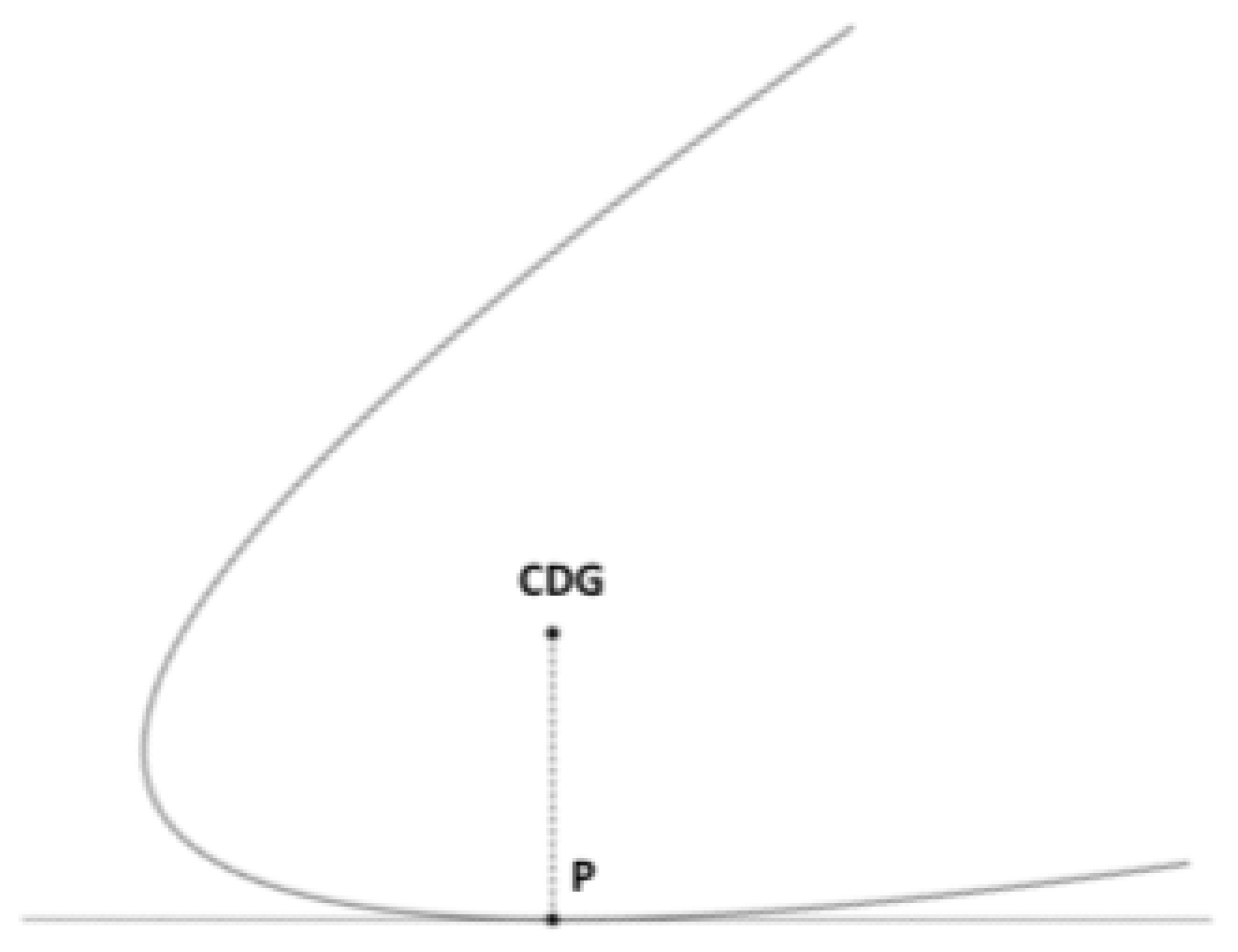
3.1.2. Application 2: Euler’s Arc

The second example, explained in session 3, is an application of Thom’s catastrophes and of Fourier and Taylor’s series.

Supposing a compressed arc (with length π) and a load m slightly off-center (ε), as it is represented in the following figure (Figure 6):

The beam resistance depends on two control parameters ($m$,$\epsilon$), which must be modelled by the Thom’s 2nd catastrophe.

Expressing the arc with the following function:

$$f\left(s\right),0\le s\le \pi$$

(9)

Fourier analysis establishes that periodic functions can be modelled by additions of harmonics of different periods. Therefore, the bean function can be expressed as an addition of sinus of different periods:

$$f\left(s\right)={\displaystyle \sum }{c}_n\sin ns$$

(10)

In this example, supposing one or two harmonics, it is obtained that:

$$m=0,\epsilon =0\Rightarrow f\left(s\right)\cong r\sin s$$

(11)

If the elastic module is $\mu =\raisebox{1ex}{$1$}\!\left/ \!\raisebox{-1ex}{$\pi $}\right.$, potential energy and elastic energy are:

$$V_P=mf\left(\frac{\pi }{2}+\epsilon \right)$$

(12)

$$V_E=\frac{1}{2\pi }{{\displaystyle \int }}_0^{\pi }{\left(f^{″}\left(s\right)\right)}^2\frac{1}{{\left(1+{\left(f^{\prime }\left(s\right)\right)}^2\right)}^3}ds$$

(13)

Applying Taylor ($\epsilon \ll$):

$$V_P=mx\cos \epsilon +mz\left(-\sin 2\epsilon \right)\cong mx\left(1-\frac{{\epsilon }^2}{2}\right)+mz\left(-2\epsilon \right)$$

(14)

The variable x depends on the variable z because the beam distance does not change when the beam distorts:

$$d={{\displaystyle \int }}_0^{\pi }\sqrt{1-{\left(f^{\prime }\left(s\right)\right)}^2}ds$$

(15)

In both cases (considering one or two harmonics) this distance is the same:

$$\begin{gathered} d={{\displaystyle \int }}_0^{\pi }\sqrt{1-{\left(r\cos s\right)}^2}ds\cong {{\displaystyle \int }}_0^{\pi }\sqrt{\left(1+\frac{1}{2}{r}^2{\cos }^{2}s+\frac{-1}{8}{r}^4{\cos }^{4}s\right)} ds= \\ =\frac{\pi }{4}\left(4-r^3-\frac{3}{16}{r}^4-\frac{5}{64}{r}^6\right) \end{gathered}$$

(16)

$$\begin{gathered} d={{\displaystyle \int }}_0^{\pi }\sqrt{1-{\left(\mathrm{xcos}s+2z\cos 2s\right)}^2}ds\cong \dots = \\ =\frac{\pi }{4}\left(4-x^2-4z^2-\frac{3}{16}{x}^4-3x^2{z}^2-\frac{5}{64}{x}^6\right) \end{gathered}$$

(17)

Equaling the two expressions below and applying Taylor approximation:

$$x\cong a_o+a_2{z}^2+a_4{z}^4⟹a_o=r,a_2=-\frac{2}{r}-\frac{3r}{4},a_4=\frac{-2}{r^3}$$

(18)

It is obtained x as an implicit function of z:

$$x\cong r+z^2\left(-\frac{2}{r}-\frac{3r}{4}\right)+z^4\frac{-2}{r^3}$$

(19)

Now we can obtain the elastic energy depending only on z:

$$V_E\cong \dots =\mathrm{constant}+\left(3+\frac{13}{8}{r}^2\right)z^2$$

(20)

The total energy is the addition of the potential and the elastic energy:

$$V=V_P+V_E\cong \mathrm{constant}-2m\epsilon z+\left(\left(3+\frac{13}{8}{r}^2\right)-m\left(\frac{2}{r}+\frac{3r}{4}\right)\right)z^2-\frac{2m}{r^3}{z}^4$$

(21)

which is the expression of the Thom’s 2nd catastrophe with vertex (supposing $\epsilon =0$):

$$m_o=(3+\frac{13}{8}{r}^2){\left(\frac{2}{r}+\frac{3r}{4}\right)}^{-1}\cong \frac{3}{2}r-\frac{1}{4}{r}^3$$

(22)

Consequently:

$$V\cong -\frac{3}{r^2}{z}^4-\frac{2}{r}\left(m-m_o\right)z^2-2r\epsilon z$$

(23)

The maxim load decreases quickly when ε increases, as it represents the Thom’s cusp represented in the following figure (Figure 7):

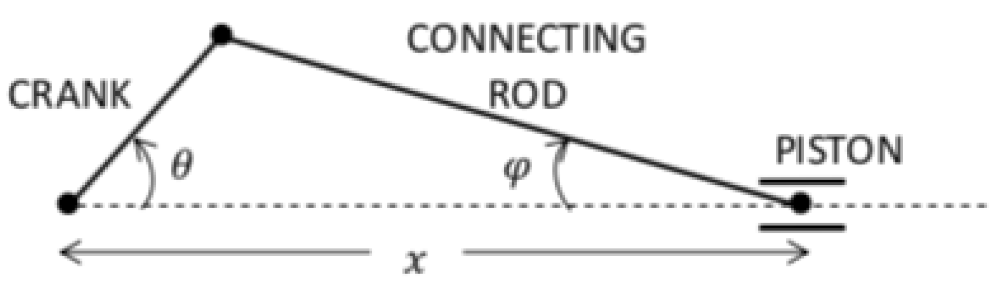
3.1.3. Application 3: Crank and Connecting Rod

This exercise, explained in session 4, is an example of the implicit function theorem, which has many applications in mechanic in order to relation the different parameters operating in a mechanism.

This application is the crank/connecting rod system of explosion motors (see Figure 8), which consists of:

• one crank moving with an angle $\theta$;
• one connecting rod whose movement depends on the crank turn;
• one piston moving horizontally on an axis.

Supposing that the crank length r and the connecting rod length L are known, this system has three position parameters:

• x: piston distance to the crank turn center;
• $\theta$: crank angle;
• $\phi$: connecting rod angle.

These three parameters are related according to the following expressions:

$$\{\begin{array}{c}x=r\cos \theta +L\cos \phi \\ r\sin \theta =L\sin \phi \end{array}$$

(24)

There are three parameters to determine the position and two equations which relate them. One of the three parameters could be expressed in function of the other two parameters and act as a control parameter determining those two parameters following the equations below.

Fixing the value of one from the three variables, we would obtain a system with two equations and two unknown factors, which would have a unique solution.

Applying the implicit function theorem:

$$\left(x,\theta ,\phi \right)\stackrel{f}{\to }\left(x-r\cos \theta -L\cos \phi ,r\sin \theta -L\sin \phi \right)$$

(25)

Calculating the derivative matrix:

$$Df=\left(\begin{array}{ccc}1& r\sin \theta & L\sin \phi \\ 0& r\cos \theta & -L\cos \phi \end{array}\right)$$

(26)

According to this theorem, one variable acts as implicit (control variable) if the minor formed by the other columns is different to zero.

If we calculate the minor of the variable x:

$$\begin{gathered} \det \left(\begin{array}{cc}r\sin \theta & L\sin \phi \\ r\cos \theta & -L\cos \phi \end{array}\right)=-rL(\sin \theta \cos \phi +\cos \theta \sin \phi )= \\ =-rL\sin \left(\theta +\phi \right)\ne 0 \mathrm{if}\left(\theta +\phi \right)\ne 0,\pi \end{gathered}$$

(27)

Therefore, x acts as a control parameter except for the neutrals:

$$\left(\theta +\phi \right)=0,\pi ⟺x=\begin{array}{c}L+r\\ L-r\end{array}$$

(28)

Indeed, the crank turn can be reversed in neutrals.

If we calculate the minor of the variable $\theta$:

$$\det \left(\begin{array}{cc}1& L\sin \phi \\ 0& -L\cos \phi \end{array}\right)=-L\cos \phi \ne 0$$

(29)

Therefore, the crank angle $\theta$ is a control parameter for all the values.

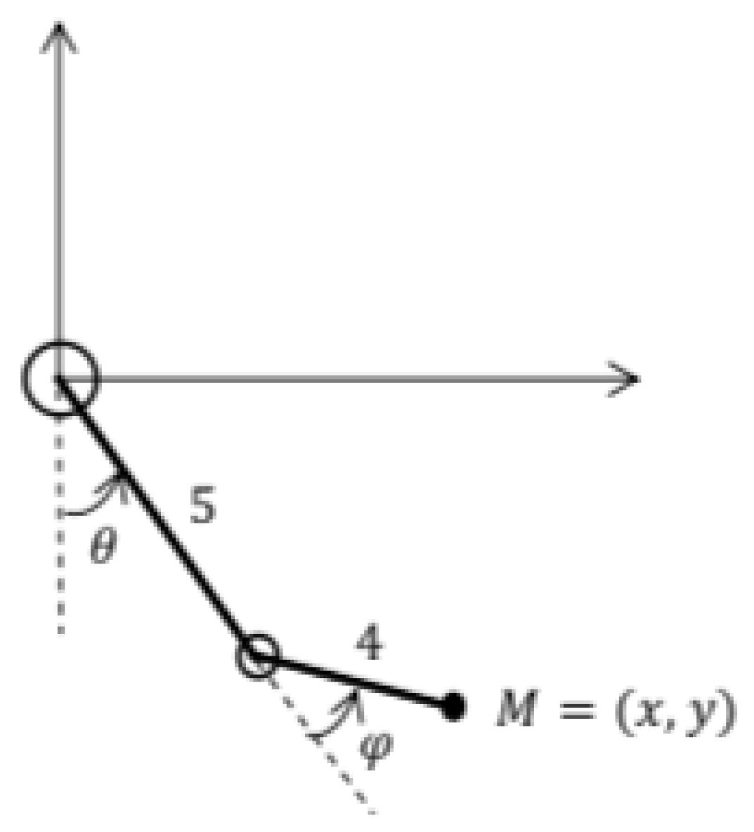
3.1.4. Application 4: Articulated Arm

However, in order to simplify the above computation and the further ones, a key tool is the matrix of the linear map. Let us obtain the matrix of f in ordinary basis.

This example, explained in session 5, is an application of inverse kinetics, which is, calculating input position, speed, etc., from outputs position, speed, etc.

This application explains the work of a robot articulated arm, whose scheme is represented in the following figure (Figure 9), which is composed by:

• a shoulder situated in the coordinates origin;
• an upper arm with length 5 and an angle $\theta >0$ from the vertical;
• an elbow situated at the end of the upper arm;
• a lower arm with length 4 and angle $\phi <\pi$ from the upper arm;
• a hand situated at the end of the lower arm, in the coordinates $\left(x,y\right)$;
• torsion motors in the articulations (the shoulder and the elbow).

The analysis consists of a direct and an inverse kinetics study of the articulated arm.

The direct kinetics study obtains the hand position from the shoulder and elbow angles, as it is calculated hereunder.

$$\left]0,\pi \right[\mathsf{𝕩}\left]0,\pi \right[\stackrel{f}{\to }\mathsf{\Omega }.$$

(30)

$$\left(\theta ,\phi \right)\stackrel{}{\to }\left(x,y\right)$$

(31)

$$\{\begin{array}{c}x=5\sin \theta +4\sin \left(\theta +\phi \right)\\ y=5\cos \theta +4\cos \left(\theta +\phi \right)\end{array}$$

(32)

The hand speed is calculated applying the chain rule, as it indicated hereunder:

$$\left(\begin{array}{c}\dot{x}\\ \dot{y}\end{array}\right)=\left(Df\right)\left(\begin{array}{c}\dot{\theta }\\ \dot{\phi }\end{array}\right),Df=\left(\begin{array}{cc}5\cos \theta +4\cos \left(\theta +\phi \right)& 4\cos \left(\theta +\phi \right)\\ -5\sin \theta -4\sin \left(\theta +\phi \right)& -4\sin \left(\theta +\phi \right)\end{array}\right)$$

(33)

what is really interesting in robots is calculating the shoulder and the elbow rotor speeds from the hand position, that is, the inverse kinetics study. To obtain these speeds, it is necessary to apply the chain rule, the inverse function theorem and the implicit function theorem, as it is carried out in the following example.

If the output is $M=\left(5,4\right)$, it is asked to obtain the shoulder and the elbow speeds $\dot{\theta }$ and $\dot{\phi }$.

It is clear to see that is a functional dependence between the hand position $\left(x,y\right)$ and the shoulder and the elbow positions $\left(\theta ,\phi \right)$ since there is only one possible triangle which determine the hand position from the shoulder and the elbow positions. Therefore

$$\mathsf{\Omega }\stackrel{f^{-1}}{\to }\left]0,\pi \right[\mathsf{𝕩}\left]0,\pi \right[$$

(34)

$$(x,y)\to \left(\theta ,\phi \right)$$

(35)

Applying the inverse function theorem, it is confirmed the $f^{-1}$ derivability:

$$\begin{gathered} \det Df=-20\cos \theta \sin (\theta +\phi )+20\sin \theta \cos \left(\theta +\phi \right)= \\ =-20\sin \left(\theta -(\theta +\phi \right))=-20\sin \phi \ne 0 \end{gathered}$$

(36)

The relation between the shoulder and the elbow speeds, and the hand speed is:

$$\left(\begin{array}{c}\dot{\theta }\\ \dot{\phi }\end{array}\right)={\left(Df\right)}^{-1}\left(\begin{array}{c}\dot{x}\\ \dot{y}\end{array}\right)$$

(37)

The hand position $M=\left(5,4\right)$ corresponds to the angles $=\frac{\pi }{2}$, $\phi =\frac{\pi }{2}$.

Replacing in the expression below, it is obtained that:

$$\left(\begin{array}{c}\dot{\theta }\\ \dot{\phi }\end{array}\right)={\left(\begin{array}{cc}4& 4\\ -5& 0\end{array}\right)}^{-1}\left(\begin{array}{c}\dot{x}\\ \dot{y}\end{array}\right)=\frac{1}{20}\left(\begin{array}{cc}0& -4\\ 5& 4\end{array}\right)\left(\begin{array}{c}\dot{x}\\ \dot{y}\end{array}\right)$$

(38)

$$\dot{\theta }=-\frac{1}{5}\dot{y}$$

(39)

$$\dot{\phi }=\frac{1}{4}\dot{x}+\frac{1}{5}\dot{y}$$

(40)

3.1.5. Application 5: Electrical Dispatch

This example, explained in session 7, is about the most important goal of engineering, which is the optimization of all the technological process.

The problem of the electrical dispatch deals with assigning the electrical central productions to the required power. All the distributions companies need to calculate the production of each supply central $P_1,\cdots ,$ $P_n$ to cover the instant demand $P$.

In each moment, it must be decided, which centrals act and with what power, considering the cost of productions of those supply centrals. The objective is reaching the minimum production cost.

The production cost of each supply electrical central is defined by the expression:

$$C_j={\alpha }_j+{\beta }_j{P}_j+{\gamma }_j{P}_j^2, 1\le j\le n,{\alpha }_j,{\beta }_j,{\gamma }_j>0$$

(41)

The problem is, if we have several supply electrical centrals which have quadratic production costs and there is a certain demand P lower than the maximum, knowing the power distribution of the different centrals and the first central that must be stopped.

To illustrate the solving of this problem, we are going to use an example with only three supply electrical centrals, whose costs are hereunder indicated:

$$C_1=7+P_1+P_1^2.$$

(42)

$$C_2=4+2P_2+2P_2^2$$

(43)

$$C_3=2+4P_3+3P_3^2$$

(44)

Total power is the three powers sum:

$$P=P_1+P_2+P_3$$

(45)

Total cost production of the three centrals is the cost productions sum:

$$\begin{gathered} C=\left(7+P_1+P_1^2\right)+\left(4+2P_2+2P_2^2\right)+ \\ +\left(2+4(P-P_1-P_2)+3{(P-P_1-P_2)}^2\right)= \\ =13+4P-3P_1-2P_2+P_1^2+2P_2^2+3{(P-P_1-P_2)}^2 \end{gathered}$$

(46)

To minimize the cost, the cost partial derivatives are calculated and equaled to zero:

$$D_{1}C=-3+2P_1-6(P-P_1-P_2)=-3-6P+8P_1+6P_2=0$$

(47)

$$D_{2}C=-2+4P_2-6(P-P_1-P_2)=-2-6P+6P_1+10P_2=0$$

(48)

The system obtained is compatible determined, therefore has a unique solution, which is:

$$\begin{array}{c}{P}_1^{*}=\frac{1}{22}\left(9+12P\right)\\ P_2^{*}=\frac{1}{22}\left(-1+6P\right)\end{array}\Rightarrow P_3^{*}=\frac{1}{22}\left(-8+4P\right)$$

(49)

This solution is valid only if $P_1^{*}$, $P_2^{*}$, $P_3^{*}\ge 0$:

$$P_1^{*}>0, \forall P$$

(50)

$$P_2^{*}>0\iff P\ge \raisebox{1ex}{$1$}\!\left/ \!\raisebox{-1ex}{$6$}\right.$$

(51)

$$P_3^{*}>0\iff P\ge 2$$

(52)

Therefore, the solution is valid only if $P\ge 2$.

If P decreases under $P=2$, the solution below is not valid. From this value, $P_3^{*}$ turns to be negative, what indicates that the third central must be the first central to stop.

In this case only the other two centrals act and the production cost is:

$$C=7+P_1+P_1^2+4+2(P-P_1)+2{(P-P_1)}^2$$

(53)

The cost derivative calculation equaled to zero is:

$$P_1^{*}=\frac{1}{6}\left(1+4P\right)$$

(54)

$$P_2^{*}=\frac{1}{6}\left(-1+2P\right)\iff \frac{1}{2}\le P\le 2$$

(55)

$$P_3^{*}=0$$

(56)

Therefore, if P decreases under $P=\frac{1}{2}$, $P_3^{*}$ turns to be negative, what indicates that the second central must stop.

In this case, the only one central which supplies power is the first central and in this case the distribution is:

$$P_1^{*}=P,P_2^{*}=P_3^{*}=0\mathrm{si}P\le \frac{1}{2}$$

(57)

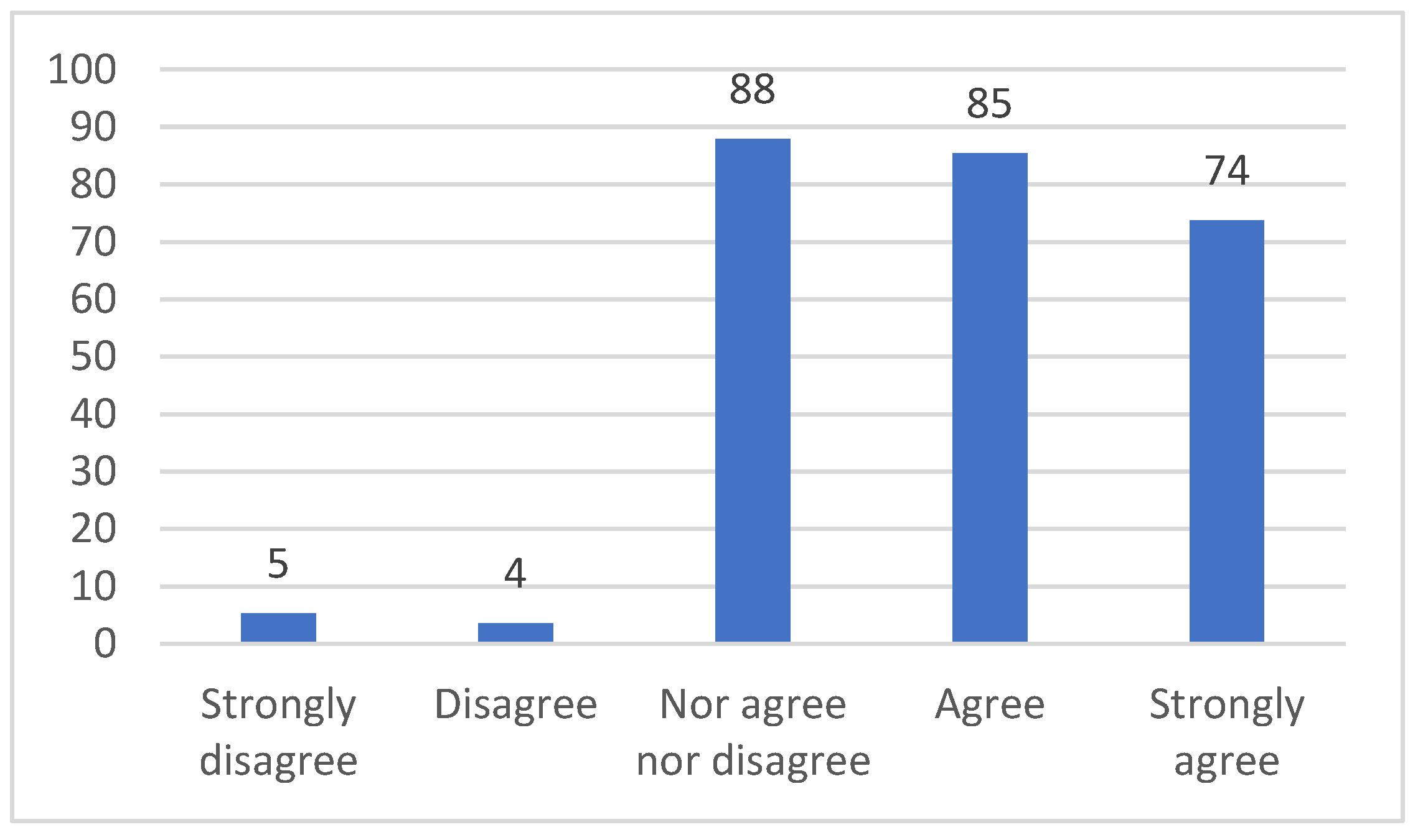
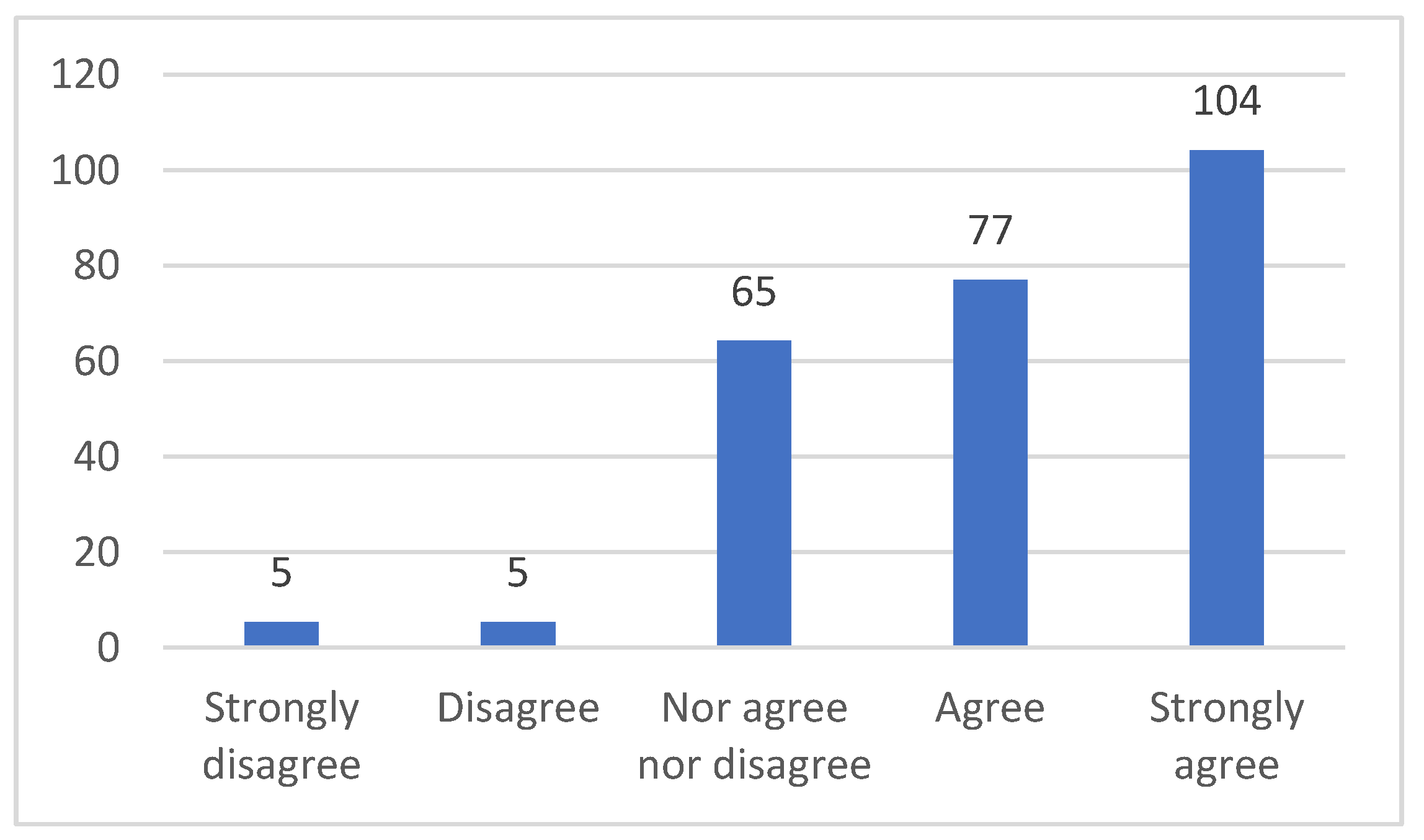
3.2. Students’ Surveys and Interviews Results

Up to now, two editions of the seminar “Application of Multivariable Calculus in Engineering” have been held, corresponding to the second semester of the 2019/2020 and 2020/2021 academic years. The contents explained in these sessions has been studied considering the answers to the anonymous questionnaires and to the personal interviews conducted to students.

Students’ surveys of the sessions undertaken until now have been analyzed. The surveys were held in the 2019/2020 and 2020/2021 academic years, after each of the sessions. The number of attending students to the sessions has been 16 and all of them have been participants in the surveys. The results obtained in these two academic years did not have relevant differences. In the following figures the answers to each question for all the sessions in both years are presented. So, for each figure, 256 represents the total number of cases, which are the answers of 16 students in each of the 8 sessions and during two academic years.

The answers to the first question (Figure 10) show that most of the students, almost 90% of the total 256 answers of students, agree with the mathematical contents developed in the sessions.

Likewise, in the answers to the second question (Figure 11), it can be observed that almost 90% of the total 256 answers of students agree with the engineering contents explained in the sessions.

According to the answers to question 3, almost 90% of the total 256 answers of students think that the sessions “Applications of Multivariable Calculus in Engineering” let them know technological applications of different mathematical concepts (Figure 12).

Almost 70% of the total 256 answers of students agree that applications of mathematical concepts achieve to increase their motivation to the subject Multivariable Calculus, as the answers to question 4 (Figure 13) show.

More than 70% of the total 256 answers of students state that the execution of practical exercises with technological applications improves the learning of mathematical concepts (Figure 14).

The response of the attending students to these sessions in 2019/2020 and 2020/2021 academic years has been very positive. As can be observed in the above figures, the number of students who agree or strongly agree with the statements about the seminar is higher than the number of students who nor agree nor disagree, except for the question 4 (Figure 13). The reason is that some students have answered that although they assess positively the contents of the seminar, they were already motivated to the study of Calculus Multivariable before attending to the seminar.

It is also worth mentioning some students’ comments expressed in the open questions asked in the anonymous surveys in both years, such as:

• These sessions let know real applications of mathematics in engineering, which gives more sense to the study of mathematics.
• Discovering that discontinuous phenomena produced in engineering processes can be modeled by mathematical theories increases the motivation towards the learning of mathematics.
• The use of mathematical concepts in technological applications, as they are implicit function theorem or Taylor and Fourier series, let students realize about the need of mathematics in engineering.
• Applications of Multivariable Calculus in mechanics and robotics increase the curiosity and the interest of students towards mathematical subjects.

The information extracted from students’ answers in personal interviews in both academic years is presented hereunder:

• The real applications shown in the sessions “Applications of Multivariable Calculus in Engineering” let students realize of the usefulness of mathematics for their degree and for their future career.
• Applications studied in this seminar have been very practical and students will use them in their future profession. Learning to solve real engineering problems shows students how essential mathematical subjects are for engineers.
• Seeing how mathematics can be applied in engineering motivates to learn mathematics in order to be able to use them in the future as engineers.
• Seeing technological applications of mathematics increases the interest towards the subject.
• These applications help students understand related mathematical concepts as the implicit function theorem, the Fourier series or the calculations of maximums and minimums in functions defined in compact sets.
• Interesting applications: Zeeman machine solved with Thom’s catastrophes theory and Taylor series and the crank/connecting rod system of explosion motors using the implicit function theorem.
• It has been very impressive knowing no technological applications of Thom’s catastrophes, such as the analysis of dogs’ behavior and sociological applications.
• Students knew that mathematics were necessary for engineering but, attending this seminar, they have discovered that mathematics are also necessary for other different disciplines.
• Mathematics are not subjects to prepare students for beginning the degree, mathematics are applications in the future work of engineers.

4. Discussion

In this work we contribute to develop an integrated STEM curriculum, introducing an implementation of mathematical applications integrated in STEM education. This study provides a connection of mathematical subjects with technological disciplines and with engineering careers, with the objective of enhancing the motivation and engagement of engineering students.

In the present engineering curriculum, the first two academic courses content very few engineering subjects, but consist of mathematics, science, communications and electives subjects. With the implementation developed in this work, mathematical subjects should cover real applications related to the main area of students enrolled degree, offering a wider view in STEM education [37,38], what would involve the improvement of the understanding and learning of mathematical concepts, as [39] states.

The main issue of this work has been the relevance of solving real and technological problems in the teaching of mathematics, since students’ analytical thinking skills are enhanced with the use of mathematical problem solving [29,30,40]. In addition, the implementation of real and practical problems in basic sciences subjects promote student engagement and motivation in STEM degrees [14,19,20,21]. Considering the results shown in Figure 13, it can be seen that almost the 70% of the total 256 answers of students agree that applications of mathematical concepts achieve to increase their motivation to the subject of Multivariable Calculus, what will lead to reduce dropout, since it is connected to motivation [14], student achievement [17] and academic performance [11]. In the results of Figure 14, it has been shown that according to more than the 70% of the total 256 answers of students, the applications explained in the seminar, let them learn mathematical concepts trough practical examples. This fact increases their motivation to mathematics, as it is confirmed in previous studies such as [28]. In addition, as shows Figure 12, almost the 90% of the total 256 answers of students state that with this sessions they have known multiple real application of Multivariable Calculus in engineering and other disciplines, what attain to encourage and motivate them to the learning of the subject, as it was analyzed in several studies [14,19,20].

The answers to the questions taken to the students in the personal interviews after the sessions “Applications of Multivariable Calculus in Engineering”, show that most of the practical problems have impressed students because they have discovered that Multivariable Calculus have applications in many different areas. Moreover, it is to highlight that for students is really motivating to know what they will be capable to do in the next academic courses, using the concepts of Multivariable Calculus. They also realized of how essential Multivariable Calculus is for their future career and increased their interest towards the subject.

The results obtained in this study support that this experience contribute to an improvement of students’ learning of mathematical concepts, as it was concluded in [33], which involves the increase of students’ performance in mathematical subjects of engineering degrees, as it was studied in previous works such as [25].

5. Conclusions

This study was carried out at the Universitat Politècnica de Catalunya-BarcelonaTech (UPC), a university focused on STEM fields. The work is based on the teaching of Multivariable Calculus by the execution of real and technological applications where Calculus concepts are necessary to solve them. The aim of this work is to generate and integrated STEM curriculum, presenting a contribution about the relationship among mathematical applications and STEM education. The work provides evidence that it is possible to increase students’ motivation through the implementation of engineering applications in the learning of mathematics, what could imply an improvement of the learning of mathematics and therefore, an increase of students’ performance and a decrease of the dropout in the first academic courses of engineering degrees. This entails a rise of interest in STEM degrees, which are essential for the economic growth of technological countries.

In view of the success of the seminar “Applications of Multivariable Calculus in Engineering”, more real applications are planned to be developed. These sessions are going to be repeated in the second semester of the next academic year 2021/2022. Likewise, the seminar “Applications of Linear Algebra in Engineering” is going to be repeated in the first semester of the next academic year. These two seminars cover the most mathematical subjects of the first academic course in engineering degrees.

It is also planned to conduct surveys and interviews to the students attending the seminar of the following academic year with the aim of collecting a greater sample of surveys results and more information about students’ experience in these sessions.

With the results obtained, it is expected that the contents developed in this work will be included in a future adaptation of mathematical subjects’ syllabus in engineering degrees.

References

1. Joyce, A. Stimulating interest in STEM careers among students in Europe: Supporting career choice and giving a more realistic view of STEM at work. European Schoolnet Brussels. 2014. Available online: https://www.educationandemployers.org/wp-content/uploads/2014/06/joyce_-_stimulating_interest_in_stem_careers_among_students_in_europe.pdf (accessed on 29 October 2021).
2. Marra, R.M.; Rodgers, K.A.; Shen, D.; Bogue, B. Leaving Engineering: A Multi-Year Single Institution Study. J. Eng. Educ. 2012, 101, 6–27. [Google Scholar] [CrossRef]
3. Caprile, M. Encouraging STEM studies Labour Market Situation and Comparison of Practices Targeted at Young People in Different Member States. Policy Dep. A 2015, 12. Available online: https://www.europarl.europa.eu/RegData/etudes/STUD/2015/542199/IPOL_STU (accessed on 29 October 2021).
4. Vennix, J.; Brok, P.D.; Taconis, R. Do outreach activities in secondary STEM education motivate students and improve their attitudes towards STEM? Int. J. Sci. Educ. 2018, 40, 1263–1283. [Google Scholar] [CrossRef] [Green Version]
5. Timms, M.; Moyle, K.; Weldon, P.; Mitchell, P. Challenges in STEM Learning in Australian Schools. Policy Insights. May 2018. Available online: https://research.acer.edu.au/policyinsights/7 (accessed on 9 August 2021).
6. Fadzil, H.M.; Saat, R.M.; Awang, K.; Adli, D.S.H. Students’ Perception of Learning Stem-Related Subjects through Scientist-Teacher-Student Partnership (STSP). J. Balt. Sci. Educ. 2019, 18, 537–548. [Google Scholar] [CrossRef] [Green Version]
7. Ministerio de Universidades. Datos y Cifras del Sistema Universitario Español; Ministerio de Universidades: Madrid, Spain, 2021.
8. Bradburn, E.; Washington, D. Short-Term Enrollment in Postsecondary Education: Student Background and Institutional Differences in Reasons for Early Departure; U.S. Department of Education, Institute of Education for Education Statistics: Washington, DC, USA, 2002. [Google Scholar]
9. Zumbrunn, S.; McKim, C.; Buhs, E.S.; Hawley, L.R. Support, belonging, motivation, and engagement in the college classroom: A mixed method study. Instr. Sci. 2014, 42, 661–684. [Google Scholar] [CrossRef]
10. Lopez, D. Using Service Learning for Improving Student Attraction and Engagement in STEM Studies. Eduction Excell. Sustain. 2017, 28, 1053–1060. [Google Scholar]
11. Wilson, D.; Jones, D.; Bocell, F.; Crawford, J.; Kim, M.J.; Veilleux, N.; Floyd-Smith, T.; Bates, R.; Plett, M. Belonging and Academic Engagement Among Undergraduate STEM Students: A Multi-institutional Study. Res. High. Educ. 2015, 56, 750–776. [Google Scholar] [CrossRef]
12. Kuh, G.D.; Cruce, T.M.; Shoup, R.; Kinzie, J.; Gonyea, R.M. Unmasking the Effects of Student Engagement on First-Year College Grades and Persistence. J. High. Educ. 2016, 79, 540–563. [Google Scholar] [CrossRef]
13. Tinto, V. Dropout from Higher Education: A Theoretical Synthesis of Recent Research. Rev. Educ. Res. 1975, 45, 89. [Google Scholar] [CrossRef]
14. Gasiewski, J.A.; Eagan, K.; Garcia, G.A.; Hurtado, S.; Chang, M.J. From Gatekeeping to Engagement: A Multicontextual, Mixed Method Study of Student Academic Engagement in Introductory STEM Courses. Res. High. Educ. 2011, 53, 229–261. [Google Scholar] [CrossRef] [Green Version]
15. Pantziara, M.; Philippou, G.N. Students’ Motivation in the Mathematics Classroom. Revealing Causes and Consequences. Int. J. Sci. Math. Educ. 2014, 13, 385–411. [Google Scholar] [CrossRef]
16. Ng, B.L.L.; Liu, W.C.; Wang, J. Student Motivation and Learning in Mathematics and Science: A Cluster Analysis. Int. J. Sci. Math. Educ. 2015, 14, 1359–1376. [Google Scholar] [CrossRef]
17. Handelsman, M.M.; Briggs, W.L.; Sullivan, N.; Towler, A. A Measure of College Student Course Engagement. J. Educ. Res. 2005, 98. [Google Scholar] [CrossRef]
18. Floyd-Smith, T.; Wilson, D.; Campbell, R.; Bates, R.; Jones, D.; Peter, D.; Plett, M.; Scott, E.; Veilleux, N. A Multi Institutional Study of Connection, Community and engagement in Stem Education: Conceptual Model Development. In Proceedings of the ASEE (American Society for Engineering Education) Conference, Arlington, VA, USA, 20 June 2020. [Google Scholar]
19. Bahamonde, A.D.C.; Aymemí, J.M.F.; Urgellés, J.V.G.I. Mathematical modelling and the learning trajectory: Tools to support the teaching of linear algebra. Int. J. Math. Educ. Sci. Technol. 2016, 48, 1–15. [Google Scholar] [CrossRef]
20. Kandamby, T. Enhancement of learning through field study. JOTSE 2018, 8, 408–419. Available online: https://dialnet.unirioja.es/servlet/articulo?codigo=6623129&info=resumen&idioma=ENG (accessed on 5 August 2021). [CrossRef] [Green Version]
21. Doerr, H.M. What Knowledge Do Teachers Need for Teaching Mathematics through Applications and Modelling? In Modelling and Applications in Mathematics Education; Springer: Boston, MA, USA, 2007; pp. 69–78. [Google Scholar] [CrossRef]
22. Chalmers, C.; Carter, M.; Cooper, T.; Nason, R. Implementing “Big Ideas” to Advance the Teaching and Learning of Science, Technology, Engineering, and Mathematics (STEM). Int. J. Sci. Math. Educ. 2017, 15, 25–43. [Google Scholar] [CrossRef] [Green Version]
23. Fan, S.-C.; Yu, K.-C.; Lin, K.-Y. A Framework for Implementing an Engineering-Focused STEM Curriculum. Int. J. Sci. Math. Educ. 2020, 19, 1523–1541. [Google Scholar] [CrossRef]
24. Perdigones, A.; Gallego, E.; García, N.; Fernández, P.; Pérez-Martín, E.; del Cerro, J. Physics and Mathematics in the Engineering Curriculum: Correlation with Applied Subjects. Int. J. Eng. Educ. 2014, 30, 1509–1521. [Google Scholar]
25. Freeman, S.; Eddy, S.L.; McDonough, M.; Smith, M.K.; Okoroafor, N.; Jordt, H.; Wenderoth, M.P. Active learning increases student performance in science, engineering, and mathematics. Proc. Natl. Acad. Sci. USA 2014, 111, 8410–8415. [Google Scholar] [CrossRef] [Green Version]
26. Borda, E.; Schumacher, E.; Hanley, D.; Geary, E.; Warren, S.; Ipsen, C.; Stredicke, L. Initial implementation of active learning strategies in large, lecture STEM courses: Lessons learned from a multi-institutional, interdisciplinary STEM faculty development program. Int. J. STEM Educ. 2020, 7, 1–18. [Google Scholar] [CrossRef]
27. Loyens, S.M.M.; Magda, J.; Rikers, R. Self-Directed Learning in Problem-Based Learning and its Relationships with Self-Regulated Learning. Educ. Psychol. Rev. 2008, 20, 411–427. [Google Scholar] [CrossRef] [Green Version]
28. Cetin, Y.; Mirasyedioglu, S.; Cakiroglu, E. An Inquiry into the Underlying Reasons for the Impact of Technology Enhanced Problem-Based Learning Activities on Students’ Attitudes and Achievement. Eurasian J. Educ. Res. 2019, 19, 1–18. [Google Scholar] [CrossRef] [Green Version]
29. Mallart, A.; Font, V.; Diez, J. Case Study on Mathematics Pre-service Teachers’ Difficulties in Problem Posing. Eurasia J. Math. Sci. Technol. Educ. 2018, 14, 1465–1481. [Google Scholar] [CrossRef]
30. Darhim, D.; Prabawanto, S.; Susilo, B.E. The Effect of Problem-based Learning and Mathematical Problem Posing in Improving Student’s Critical Thinking Skills. Int. J. Instr. 2020, 13, 103–116. [Google Scholar] [CrossRef]
31. Passow, H.J. Which ABET Competencies Do Engineering Graduates Find Most Important in their Work? J. Eng. Educ. 2012, 101, 95–118. [Google Scholar] [CrossRef]
32. López-Díaz, M.; Peña, M. Contextualization of basic sciences in technological degrees. FIE2020-Front. Educ. 2020, 1–5. Available online: https://upcommons.upc.edu/handle/2117/334379 (accessed on 29 October 2021).
33. Lacuesta, R.; Palacios, G.; Fernandez, L. Active learning through problem based learning methodology in engineering education. In Proceedings of the 2009 39th IEEE Frontiers in Education Conference, San Antonio, TX, USA, 18 October 2009; pp. 1–6. [Google Scholar] [CrossRef]
34. Chen, J.; Kolmos, A.; Du, X. Forms of implementation and challenges of PBL in engineering education: A review of literature. Eur. J. Eng. Educ. 2020, 46, 90–115. [Google Scholar] [CrossRef]
35. Chávez, D.A.; Sánchez, V.M.G.; Vargas, A.C. Problem-based learning: Effects on academic performance and perceptions of engineering students in computer sciences. JOTSE 2020, 10, 306–328. Available online: https://dialnet.unirioja.es/servlet/articulo?codigo=7641626&info=resumen&idioma=ENG (accessed on 5 August 2021).
36. López-Díaz, M.; Peña, M. Mathematics Training in Engineering Degrees: An Intervention from Teaching Staff to Students. Mathematics 2021, 9, 1475. [Google Scholar] [CrossRef]
37. Kertil, M.; Gurel, C. Mathematical Modeling: A Bridge to STEM Education. Int. J. Educ. Math. Sci. Technol. 2016, 4, 44. [Google Scholar] [CrossRef]
38. Yıldırım, B.; Sidekli, S. Stem applications in mathematics education: The effect of stem applications on different dependent variables. J. Balt. Sci. Educ. 2018, 17, 200–214. [Google Scholar] [CrossRef]
39. Kumar, S.; Jalkio, J.A. Teaching Mathematics from an Applications Perspective. J. Eng. Educ. 1999, 88, 275–279. [Google Scholar] [CrossRef] [Green Version]
40. Van Der Wal, N.J.; Bakker, A.; Drijvers, P. Which Techno-mathematical Literacies Are Essential for Future Engineers? Int. J. Sci. Math. Educ. 2017, 15, 87–104. [Google Scholar] [CrossRef] [Green Version]
Figure 1. Centre of gravity.
Mathematics 10 00341 g001
Figure 2. Position of the center of gravity.
Mathematics 10 00341 g002
Figure 3. Stability of the center of gravity.
Mathematics 10 00341 g003
Figure 4. Cusp curve.
Mathematics 10 00341 g004
Figure 5. Machine behavior.
Mathematics 10 00341 g005
Figure 6. Compressed arc.
Mathematics 10 00341 g006
Figure 7. Thom’s cusp.
Mathematics 10 00341 g007
Figure 8. Crank/connecting rod system.
Mathematics 10 00341 g008
Figure 9. Articulated arm.
Mathematics 10 00341 g009
Figure 10. Answers to question 1: The assessment of mathematical contents is positive.
Mathematics 10 00341 g010
Figure 11. Answers to question 2: The assessment of engineering contents is positive.
Mathematics 10 00341 g011
Figure 12. Answers to question 3: The sessions “Applications of Multivariable Calculus in Engineering” let students know technological applications of different mathematical concepts.
Mathematics 10 00341 g012
Figure 13. Answers to question 4: The applications of mathematical concepts achieve to increase the motivation to the subject Multivariable Calculus.
Mathematics 10 00341 g013
Figure 14. Answers to question 5: The execution of practical exercises with technological applications improve the learning of mathematical concepts.
Mathematics 10 00341 g014