Latin American Agri-Food Exports, 1994–2019: A Gravity Model Approach

Abstract

This study analyses the causes of the strong growth in the agri-food exports of Latin America between 1994 and 2019. To do this, a series of gravity models are estimated, using as a dependent variable the agri-food exports of 15 Latin American countries to their 185 principal trading partners. The empirical specification is based on the gravity theory of trade, according to which, trade between two countries is determined by the size of both of their markets and their transport costs. Other variables have also been included, considering the theoretical foundations proposed for the gravity model. We initially used the PPML estimator since it is the method that provides estimates with the best properties. We later compared these results with those obtained through OLS and the Heckman selection model. Our findings show that the growth in agri-food exports is explained by factors of both supply and demand, but that the latter plays a more important role since we have obtained evidence of a reverse home-market effect. Furthermore, we can conclude that the creation of regional trade agreements, such as NAFTA, MERCOSUR, CACM, APEC, and TPP, has significantly favoured agri-food exports in the region.

1. Introduction

In the second half of the twentieth century, profound changes took place in global trade. One of the most important was the growth in the trade of manufactured goods between developed countries, replacing the pattern of inter-industrial trade that arose during the first wave of globalization [1]. Consequently, although the trade of agricultural and food products was growing faster than ever, its share of total trade fell significantly due to the fall in its relative prices and the growing participation of manufactured products [2]. The Latin American countries lost an important part of their relative weight in the global exports of agricultural and food products between 1950 and 1990, although they did not become prominent players in the global trade of manufactured goods either. This loss of share was due not only to the change in the region’s development model towards import substitution and its bias against agricultural exports, but also to the specialisation in products with a weak demand and low level of industrial transformation. The agricultural protectionism of the developed countries and the failure of their regional integration processes, in contrast to Europe’s success in this respect, were also contributing factors [3]. However, from the mid-1990s, Latin American exports of agri-food products grew substantially, giving rise to what has been dubbed as an agricultural export boom and a “re-primarization” of its economies.

Within this context, the objective of this article is to analyse the determinants of this change in trend, which led to strong growth in agri-food exports from Latin America between 1994 and 2019. This time horizon, which is sufficiently broad, allows us to address the crucial decades of change in Latin American agri-food trade patterns when Latin America was reintegrated into international trade and the structural reforms known as the Washington Consensus were implemented. To do this, we have used econometric models derived from the gravity equation. Given that there is an important debate regarding the most appropriate method of estimation, we have performed the following three alternative methods: the Poisson pseudo maximum likelihood (PPML), ordinary least squares (OLS), and the Heckman sample selection model. The estimates require the construction of a database of bilateral trade, for which we have used information provided by COMTRADE.

This study contributes to the existing empirical literature on international trade as, to the best of our knowledge, there are no other studies that have the objective of explaining the strong expansion in recent decades of the agri-food exports of the whole of Latin America for such a broad time horizon and with a methodology that uses econometric models for this purpose. Some similar research has been conducted for the decades prior to those covered in this article [3,4]. Other studies have provided interesting data for analyzing the agri-food trade of Latin America or some of its countries for part of the period studied in this article [5,6,7]. This study seeks to fill that research gap.

Our results show that the growth in agri-food exports can be explained by factors of both supply and demand, but that the latter plays a more important role, with a reverse home-market effect. Furthermore, we can conclude that the creation of regional trade agreements, such as the North American Free Trade Agreement (NAFTA), the Southern Common Market (MERCOSUR), the Central American Common Market (CACM), the Asia-Pacific Economic Cooperation (APEC), and the Trans-Pacific Partnership (TPP), has significantly favoured agri-food exports. We can also confirm that the PPML estimation method is the most appropriate estimator as it is robust to heteroskedasticity, which is frequent in trade models and when there is a high number of zero values, as in our case.

The rest of the paper is structured as follows: the next section explains the materials and methods used. It begins by explaining the evolution of Latin American agri-food exports, then describes the theoretical framework, the methods of estimation, and the empirical model and data used. The third section presents the results and their discussion. The following section is a sensitivity analysis using alternative estimation methods. Finally, the article closes with our main conclusions.

2. Materials and Methods

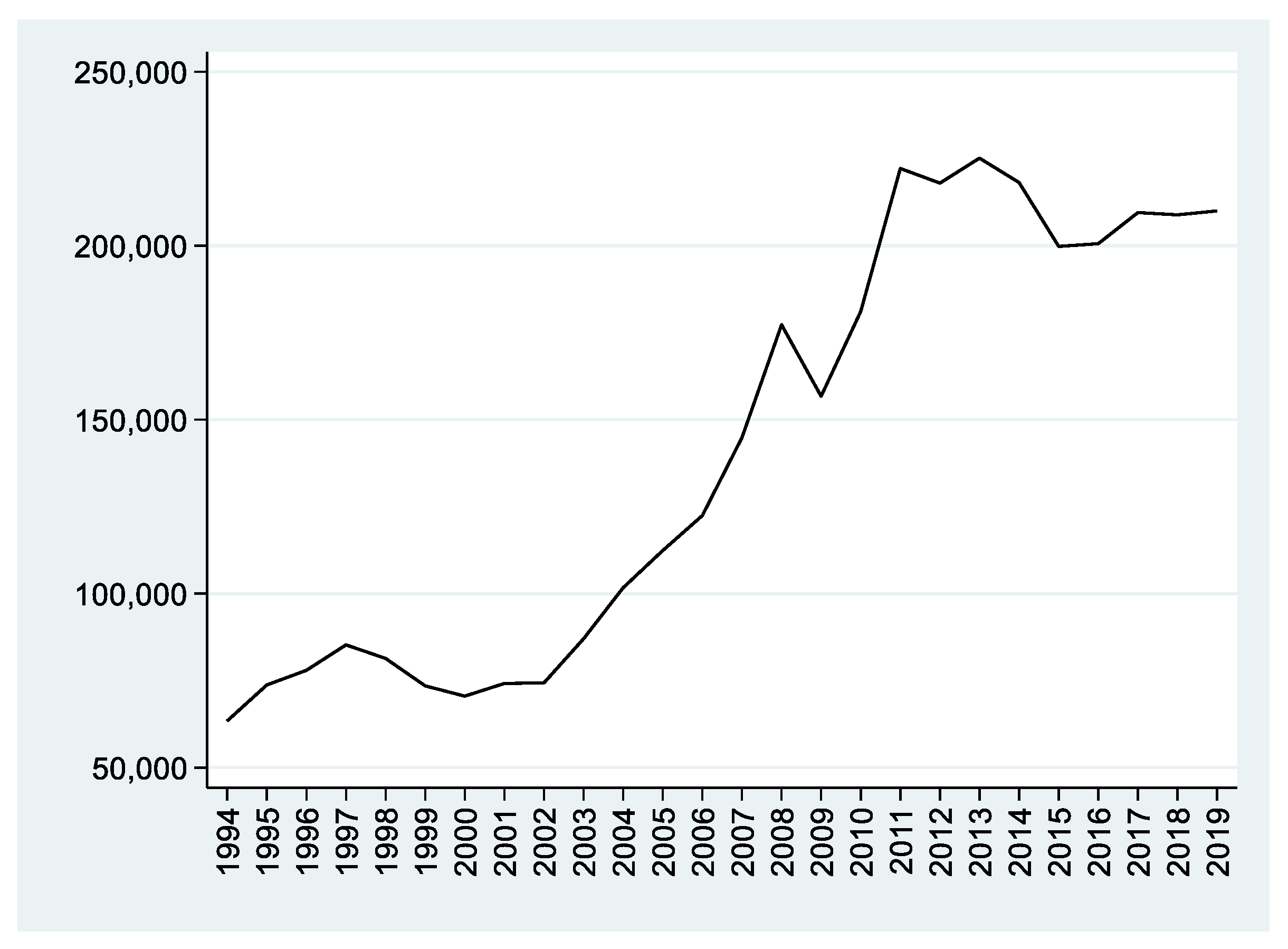
2.1. The Evolution of Agri-Food Exports from Latin America, 1994–2019

The export of basic products has traditionally been considered as one of the fundamental factors driving Latin American economic development during the first globalization [8]. In some countries, the dynamism of the so-called export-led model produced a significant improvement in living standards. In others, however, the concentration of exports in a single product and in a single market, with very few linkages with the non-export sector, meant that the impact on economic growth was limited [9,10,11]. However, from 1950, the protectionism and promotion of industry formed the foundation of the new import substitution industrialisation model (ISI) [12]. This model not only made the manufacturing industry the axis of economic development, but was also characterized by a greater state intervention and a strong orientation of the economy towards the domestic market [13]. This change in development model, the specialization of the region in low-income elasticity agri-food products, the failure of the regional integration processes, and the protectionism of developed countries caused the agri-food exports from Latin America between 1960 and 1990 to experience comparatively low growth with respect to the rest of the world. Hence, the participation of the region in the world’s total fell significantly [3]. Agriculture tended to be oriented more towards the domestic market, which was growing strongly as a result of the demographic transition experienced by the countries of the region. Growth in agricultural production was moderate [14].

The external debt crisis of the 1980s led to a shift towards a more open growth model, with significant market reforms in the 1990s and the promotion of the diversification of exports, which once again boosted agri-food exports [4]. The new strategy consisted of mobilizing resources in competitive export sectors, including agriculture. Thus, the penalization of exportable agricultural products as a result of the ISI policies was drastically reduced after 1993 [14]. From 1992, agricultural production and productivity grew at the fastest rate of the entire second half of the twentieth century [15]. The percentage of agricultural production exported also increased, from just under 30% before 1992 to around 40% in the final years of the century [14].

The increase in the prices of basic products, which began in 2003 and lasted practically for a decade, generated what the Economic Commission for Latin America and the Caribbean (ECLAC) called a “re-primarization”, understood as a renewed and growing participation of natural resources in exports. This re-primarization was reinforced by the increase in trade with China, which has become the most important trading partner of the region. Currently, the Latin American agricultural sector continues to play an influential role in the economic growth of this region, although, despite the improvements that have occurred since the second half of the twentieth century, this sector is still a long way from equalling the levels of productivity of developed countries [14].

In the period analysed, between 1994 and 2019, the international trade of agri-food products from Latin America grew substantially. In 1994, the value of the exports of these products amounted to 63,424 billion 2015 USD, while in the year 2019 they were worth 210,012 billion 2015 USD. These figures indicate that foreign sales were growing at an accumulative annual average rate of 4.71%. As we can observe in Figure 1, at the end of the period, agri-food trade had multiplied 3.3 times. It is evident that such a significant growth in the exports of highly natural resource-intensive products has had very varied implications, both from the point of view of sustainability and its effects on economic development [16,17,18,19,20].

2.2. Theoretical Framework: Gravity Models and the Determinants of International Trade

Gravity models have been widely used to analyse the determinants of international trade. Today, they have become the workhorse of the applied international trade literature. Their success is partly due to the fact that they are highly intuitive models as, based on Newton’s universal law of gravitation, they estimate that the international trade between two countries is directly proportional to the product of their sizes in economic terms and inversely proportional to the trade frictions between them. Another reason for their success is their high explanatory power, as empirical studies that use them are able to explain between 60 and 90 per cent of the variation with aggregate data as well as with sectoral data for both goods and services [21]. However, even though the gravity equation was considered an empirical success, it was often criticized for lacking sound theoretical foundations, but the emergence of the new international trade theory provided it with a rigorous theoretical basis [22,23,24,25].

Analogous to Newtonian physics, the gravity equation establishes that the trade flow from country $\mathrm{i}$ to country $\mathrm{j}$, denoted by ${\mathrm{X}}_{\mathrm{ij}}$, is proportional to the product of their GDPs, ${\mathrm{Y}}_{\mathrm{i}}$ and ${\mathrm{Y}}_{\mathrm{j}}$, and inversely proportional to the distance between them, ${\mathrm{D}}_{\mathrm{ij}}$, which, in general terms, is used as a proxy of the transport and information costs and constitutes an obstacle to trade. That is as follows:

$${\mathrm{X}}_{\mathrm{ij}}=\mathrm{C}\frac{{\mathrm{Y}}_{\mathrm{i}}{\mathrm{Y}}_{\mathrm{j}}}{{\mathrm{D}}_{\mathrm{ij}}}{=\mathrm{FG}}_{\mathrm{ij}}$$

(1)

where $\mathrm{FG}$ is the gravitational force (international trade) between two objects (countries) $\mathrm{i}$ $\mathrm{j}$; $\mathrm{C}$ is the gravitational constant; ${\mathrm{Y}}_{\mathrm{i}}$ and ${\mathrm{Y}}_{\mathrm{j}}$ are the masses (sizes) of the object (country) $\mathrm{i}$ $\mathrm{j}$; $\mathrm{D}$ is the distance (trade frictions) between the two objects (countries) $\mathrm{i}$ $\mathrm{j}$. These models predict that the pairs of the largest countries trade more, but the countries with the greatest distance between one another trade less, perhaps because the transport costs between them are higher.

The simplest econometric model derived from this equation can be expressed as follows:

$${\mathrm{X}}_{\mathrm{ij}}{=\mathsf{\alpha }}_0{\mathrm{Y}}_{\mathrm{i}}^{\mathsf{\alpha }1}{\mathrm{Y}}_{\mathrm{j}}^{\mathsf{\alpha }2}{\mathrm{D}}_{\mathrm{ij}}^{\mathsf{\alpha }3}{\mathsf{\epsilon }}_{\mathrm{ij}}$$

(2)

The model expressed in Equation (2), is normally linearised by taking logarithms and estimating the parameters of interest by OLS, giving rise to the following equation:

$${\mathrm{logX}}_{\mathrm{ij}}{=\mathsf{\alpha }}_0^{\ast }{+\mathsf{\alpha }}_1{\mathrm{logY}}_{\mathrm{i}}{+\mathsf{\alpha }}_2{\mathrm{logY}}_{\mathrm{j}}{+\mathsf{\alpha }}_3{\mathrm{logD}}_{\mathrm{ij}}{+\log \mathsf{\epsilon }}_{\mathrm{ij}}$$

(3)

where ${\mathsf{\alpha }}_0^{\ast }=\ln \left({\mathsf{\alpha }}_0\right)$ is the constant of the equation and the rest of the coefficients refer to the elasticities of the trade flows with respect to each regressor.

This model does not take into account the effect that many other variables can have on the trade between two countries. Therefore, it is necessary to expand it with other variables.

This model was an empirical success, but it does not have a theoretical justification, as pointed out by Yotov et al. [21]. The first modern derivation of the gravity equation with a theoretical underpinning can be found in Anderson [22]. This author derived a simple gravity equation, assuming a world without trade costs and with homothetic preferences. He also derived several models considering trade costs. One of the most cited models is the Armington model. This model assumes that each country is the only source of production of each good (the so-called Armington assumption). Trade costs are modeled as “iceberg costs”, meaning that, for each good, a certain fraction melts away in the trading process. Consumer preferences are characterized by a constant elasticity of substitution (CES) utility function. Bergstrand [26] modifies the Anderson framework [22] and includes a nested CES demand structure where the elasticity of substitution among imported goods can differ from the elasticity of substitution between domestically produced goods and imported goods. Unlike Anderson [22], Bergstrand [26] assumed that there are costs associated with distributing the products to each potential market and this cost could be modeled with a constant elasticity of transformation (CET) function. The idea is that output produced for one destination cannot be costlessly transformed into output for a different destination.

As Baier and Standaert [27] point out, one weakness of the Armington model of Anderson [22] and Bergstrand [26] was that product differentiation was determined arbitrarily depending on the country of origin. Krugman [28], Krugman [29], and Helpman and Krugman [30] proposed new models with a more complex supply-side model of production. These models have a monopolistic competitive market structure, consumers have a preference for “love of variety”, and firms within a country all have the same production technology, which, for each firm, exhibits increasing returns to scale.

Arkolakis et al. [31] and Baier and Standaert [27] demonstrated that all these proposed models generate a similar structural gravity equation as follows:

$${\mathrm{X}}_{\mathrm{ij}}=\mathrm{G}{\left(\frac{{\mathrm{t}}_{\mathrm{ij}}}{{\Pi }_{\mathrm{i}}{\mathrm{P}}_{\mathrm{j}}}\right)}^{-\mathsf{ϵ}}{\mathrm{Y}}_{\mathrm{i}}{\mathrm{E}}_{\mathrm{j}}$$

(4)

where G is a constant term, t_ij are trade costs between countries i and j; ${\mathrm{Y}}_{\mathrm{i}}$ is the production in country i; ${\mathrm{E}}_{\mathrm{j}}$ is total expenditure of country j; ϵ is the trade elasticity; ${\Pi }_{\mathrm{i}}$ and ${\mathrm{P}}_{\mathrm{j}}$ are the exporter and importer price indexes that aggregate the trade costs over all trading partners.

Anderson and van Wincoop [32] refer to these price terms as the multilateral trade resistance terms (MTRs). The outward multilateral resistance terms, ${\Pi }_{\mathrm{i}}$, allow us to take into account the fact that the bilateral exports of one country $\mathrm{i}$ to another $\mathrm{j}$ depend on the trade costs of all the export markets, and the inward multilateral resistance terms, ${\mathrm{P}}_{\mathrm{j}}$, allow us to take into account the dependence of imports into country $\mathrm{i}$ from country $\mathrm{j}$ on the trade costs of all the possible suppliers. These authors argued that the traditional gravity model was not correctly specified and that previous gravity model estimation results could lead to biased inferences as they omitted the MTRs that can be important for considerations of heterogeneity. These MTRs for the importer and exporter constitute trade barriers that are non-observable or difficult to measure. Baldwin and Taglioni [33] remark the importance of treating these multilateral resistance terms properly, and, over the years, researchers have proposed alternative ways of proxying the MTRs. Now, one of the most accepted approaches in applied research consists of using country-fixed effects for importers and exporters and year-fixed effects to account for the MTRs in a panel [33,34,35].

The inclusion of these variables, together with other proxies of the trade costs between countries, such as a common language, common border, etc., in addition to distance, solves the problems associated with the simplest atheoretical model, which causes biases due to the omission of relevant variables.

More recently, several models have been presented using alternative assumptions about the utility function [36], the modelization of the trade cost or models that include intermediate goods used in the production process [37,38] and when several sectors are considered, a sectoral gravity model is also used [39,40].

2.3. Methods of Estimation

The theoretical foundation of the gravity model is no longer in doubt since the emergence of the new trade theory, but the current debate focuses on the determination of the most suitable estimation technique. As is usual in trade data, heteroskedasticity is a frequent problem and the econometric method selected should be robust to different patterns of heteroskedasticity. An additional problem in the applied international trade literature is that not all countries trade all products with all partners and, consequently, there are many zero trade values in most current trade datasets, so the estimator method has to take into account the information contained in these flows.

Traditionally, the multiplicative gravity model has been linearized through a logarithmic transformation and estimated by OLS. Nonetheless, when the log-linear gravity model (3) or the log-linear transformation of (4) is estimated by OLS, two fundamental problems arise. The first is the possible bias in the estimates of the parameters associated with truncation generated because the observations of zero where exports from one country to another are not taken into account. The second problem arises when the perturbation of the model is heteroskedastic and depends on one of the variables of the model, then $\mathrm{E}\left[\ln \left({\mathsf{\epsilon }}_{\mathrm{ijt}}\right)\right]$ will depend on the variance of ${\mathsf{\epsilon }}_{\mathrm{ijt}}$ and the hypothesis of exogeneity will not be maintained, leading to inconsistent estimates of the elasticity coefficients. This is because a logarithmic transformation of the gravity model changes the properties of the error term due to Jensen’s inequality. In other words, the expected value of the logarithm of a random variable is different to the logarithm of its expected value.

In order to avoid the problem of truncation, which is produced in the log-linear model, one solution that has been proposed is to substitute these zeros with a small positive arbitrary value and estimate the model with OLS. However, this censoring of the data has no theoretical or empirical justification and can seriously distort the results, reducing efficiency and leading to biased and inconsistent estimates [41,42,43,44,45,46].

An alternative procedure is the two-step estimation method proposed by Heckman [47] and the extension of Helpman et al. [48], which has the objective of correcting the sample selection bias by eliminating the zero trade flows when estimating the log-linear function of the gravity equation by OLS. To do this, the following two equations are used: a selection equation, which includes the factors that determine the probability of positive trade between two countries; and an outcome equation, which takes into account the factors determining trade intensity. Helpman et al. [48] propose a theoretically founded two-step selection process where exporters must absorb certain fixed costs in order to enter a market. As is typical with Heckman-based methods, it is absolutely necessary and also challenging to find an exclusion restriction or instrumental variable that influences the extensive margin of trade (selection equation) without affecting the intensive margin of trade (outcome equation) to help identification. The idea is that due to trade costs, firms differ in productivity and only firms with productivity levels beyond a certain threshold end up exporting. It has the advantage of resolving the problem of zero trade values but is sensitive to the non-compliance of the homoscedasticity hypothesis, which can generate inconsistent estimates since heteroskedasticity is usually pervasive in most trade data, as shown by Martin and Pham [49] and Santos Silva and Tenreyro [50]. The sample selection model has also been criticized on the grounds that it is difficult to satisfy the exclusion restriction.

The zero values in the endogenous variable are not a problem if the model is estimated in its multiplicative form. Therefore, several non-linear methods have been developed to address this problem of the log-linear model.

The PPML estimator fulfils the requisites for being a consistent estimator that is reasonably efficient under heteroskedasticity and is able to take advantage of the information contained in the zero trade flows because it estimates the model in its multiplicative form using the endogenous variable in levels without log-transforming [51]. Santos Silva and Tenreyro [51] show that under weak assumptions, essentially simply that the gravity model contains the correct set of explanatory variables, the PPML estimator provides consistent estimates of the original nonlinear model.

Even though the influential study of Santos Silva and Tenreyro [51] has aroused some controversies in the literature and other alternative estimation techniques have been proposed, such as the feasible generalized least squares (FGLS), the gamma pseudo-maximum likelihood (GPML), the multinomial pseudo-maximum likelihood (MNPML), the negative binomial pseudo-maximum likelihood (NBPML), the non-linear least squares (NLS), the Tobit estimator, the zero-inflated pseudo-maximum likelihood (ZIPML), the zero-inflated binomial pseudo-maximum likelihood (NIBPML), or the zero-inflated Poisson quasi likelihood (ZINPQL) [44,46,48,49,52,53,54,55,56,57], there is currently a high-degree of consensus whereby the PPML estimator is considered the most appropriate for addressing the problem of heteroskedasticity and a large number of zero trade values [52,58,59,60,61]. Therefore, in this article, we have initially estimated our models with the PPML method because it produces consistent estimates under relatively assumptions and deals with heteroskedasticity. Nevertheless, we have also conducted a sensitivity analysis using two alternative estimation methods.

2.4. Empirical Model and Data

Our database includes the agri-food exports of 15 countries in Latin America (Argentina, Plurinational State of Bolivia, Brazil, Chile, Colombia, Costa Rica, Ecuador, El Salvador, Guatemala, Honduras, Mexico, Nicaragua, Paraguay, Peru, and Uruguay) to all of the countries in the world. The representativeness of these 15 countries selected of the total agri-food exports of Latin America during the period 1994–2019 fluctuates between 88.98% and 93.77%. The data are organised according to the Standard International Trade Classification (SITC) Revision 3 at the four-digit level, although with respect to the econometric estimate, the trade flows are aggregated according to the exporter, importer, and year. (The commodities groups included, with a disaggregation of 2, 3 and 4 digits, are as follows: 00, 01, 02, 03, 04, 05, 06, 07, 08, 09, 11, 12, 21, 22, 231, 2322, 24, 261, 263, 264, 265, 268, 2721, 2919, 292, 41, 42, and 43. We have taken into account a total of 231 products).

Given the limitations of the log-linear specification of the gravity model, the specification of the augmented gravity model to explain the exports from a Latin American country $\mathrm{i}$ of an agricultural product to another country in the world $\mathrm{j}$ used in this study is as follows:

$$\begin{gathered} {\mathrm{X}}_{\mathrm{ij},\mathrm{t}}=\exp \left[{\mathsf{\alpha }+\mathsf{\beta }}_1\ln \left({\mathrm{Y}}_{\mathrm{i},\mathrm{t}}\right){+\mathsf{\beta }}_2\ln \left({\mathrm{Y}}_{\mathrm{j},\mathrm{t}}\right){+\mathsf{\beta }}_3\ln \left({\mathrm{Dist}}_{\mathrm{ij}}\right){+\mathsf{\beta }}_4\ln \left({\mathrm{Excvol}}_{\mathrm{ij},\mathrm{t}}\right){+\mathsf{\beta }}_5\ln \left({\mathrm{Polconv}}_{\mathrm{i},\mathrm{t}}\right){+\mathsf{\beta }}_6{\mathrm{Lang}}_{\mathrm{ij}} \\ +{\mathsf{\beta }}_7{\mathrm{Landlocked}}_{\mathrm{i}}{+\mathsf{\beta }}_8{\mathrm{RTA}}_{\mathrm{ij},\mathrm{t}}{+\mathsf{\beta }}_9{\mathrm{WTO}}_{\mathrm{ij},\mathrm{t}}{+\mathsf{\theta }}_{\mathrm{i}}+{\Omega }_{\mathrm{j}}{+\mathsf{\mu }}_{\mathrm{t}}\right]{+\mathsf{\epsilon }}_{\mathrm{ij},\mathrm{t}} \end{gathered}$$

(5)

where $“\mathrm{i}”$ is the exporting country ($\mathrm{i}=1, 2, \dots , 15$), $“\mathrm{j}”$ is the importing country $\left(\mathrm{j}=1, 2,\dots , 185\right)$ and $\mathrm{t}=1994, \dots , 2019$ is the time period analysed. The years analysed are fundamental, given that the development model of Latin American countries changed from the 1990s onwards as a result of the policies implemented to overcome the deep economic crisis. Martín-Retortilo et al. [14] determined that there was a structural break in 1993 in Latin American agricultural production. We have not been able to include 1993 in our study because of the absence of data for some countries. Furthermore, $\ln$ denotes the natural logarithm of the variables. The dependent variable of the gravity equation is represented by ${\mathrm{X}}_{\mathrm{ij},\mathrm{t}}$, which are the agri-food exports of country $\mathrm{i}$ to country $\mathrm{j}$ in year $\mathrm{t}$ in real terms, in 2019 USD, taken from UN COMTRADE [61]. ${\mathrm{Y}}_{\mathrm{i},\mathrm{t}}$ and ${\mathrm{Y}}_{\mathrm{j},\mathrm{t}}$ are the real GDP, in 2019 USD, of the exporting country and the importing country, respectively, in year t, and measures the size of the market of each country, capturing the effect of the supply capacity of the exporter $\mathrm{i}$ (country of origin) and the demand capacity of the importer $\mathrm{j}$ (country of destination), respectively [62] (databases CEPII and WDI [63,64]).

${\mathrm{Dist}}_{\mathrm{ij}}$ is the geographical distance in kilometres between the capitals of the countries of origin and destination (database CEPII [63]). There is full consensus that physical distance is the best indicator of trade costs. It reflects not only higher transport costs, but is correlated with cultural differences that can delay the transfer of information and the establishment of trust [65]. Geodesic distances are used by applying the great circle formula, which takes into account the longitude and latitude of the capital of each country as a proxy for the centre of gravity. There are many efforts to improve bilateral distance measures (for more details see [66,67,68]), but the simplest and most commonly used measure is the great circle distance between capitals. Nevertheless, it is clear that this is only an approximation of the real costs of trade with the implicit assumption that distance costs are a linear function of distance. For example, no distance may be representative of countries that share long borders with goods moving across many entry points and distance cannot account for the differences in the cost of alternative means of transport.

Futhermore, in order to take into account other frictions and obstacles to trade, we have also considered a series of variables in addition to distance that could reduce trade to reflect the hypothesis that transport costs increase with distance. ${\mathrm{Excvol}}_{\mathrm{ij},\mathrm{t}}$ is an indicator of the volatility of the bilateral nominal exchange rate (between i and j) in year $\mathrm{t}$ (measured as the standard deviation in the annual natural logarithm of the bilateral nominal exchange rate, for each pair of countries, in the period of the 10 previous years to $\mathrm{t}$, drawing the exchange rate data from the World Bank [64]). ${\mathrm{Polconv}}_{\mathrm{i},\mathrm{t}}$ refers to the political uncertainty in country $\mathrm{i}$ ([69]). The effects of these three latter variables on exports are expected to be negative.

Other variables taken into account are as follows: ${\mathrm{Lang}}_{\mathrm{ij}}$ which is a dummy variable that takes the value of 1 if the countries share the same official language and 0 otherwise (database CEPII [63]), indicative of the cultural proximity between the two countries; ${\mathrm{Landlocked}}_{\mathrm{i}}$ is another dummy variable that takes the value of 1 if country $\mathrm{i}$ does not have direct access to the sea and 0 otherwise, as a measure of the facility to trade; ${\mathrm{RTA}}_{\mathrm{ij},\mathrm{t}}$ is a dummy variable that takes the value of 1 if the two countries i and j are members of the same regional trade agreement and 0 otherwise [63] and indicates whether there are preferential trading conditions between a specific pair of countries. ${\mathrm{WTO}}_{\mathrm{ij},\mathrm{t}}$ is another dummy variable that captures the impact of belonging to the World Trade Organization (WTO) and takes the value of 1 if the countries i and j both belong to the WTO and 0 otherwise [63]. A positive sign in the coefficient of the two latter dummy variables indicates trade creation and a negative sign the contrary; $\mathsf{\alpha }$ denotes the independent term, while ${\mathsf{\beta }}_{\mathrm{s}}$, ${\mathsf{\theta }}_{\mathrm{i}}$, ${\Omega }_{\mathrm{j}}$ and ${\mathsf{\mu }}_{\mathrm{t}}$ are parameters to estimate that measure the effects of each of the explanatory variables and the specific effects of each of the exporting countries $\left(\mathrm{i}\right)$, importing countries $\left(\mathrm{j}\right)$, and years $\left(\mathrm{t}\right)$, respectively.

Given that the GDP of the exporting country is a highly imperfect measure of its capacity to supply agri-food products, alternatively we have substituted this variable in the model with the gross agricultural production (collected from FAOSTAT [70]), ${\mathrm{GAP}}_{\mathrm{i},\mathrm{t}}$, to adapt the gravity equation to the specific case of agri-food trade and to measure the effect of the changes in the capacity of agricultural production on exports. The expected sign of its coefficient is also positive.

Alternatively, we have disaggregated the variable ${\mathrm{RTA}}_{\mathrm{ij},\mathrm{t}}$, by introducing several dummy variables in order to explore the effects of belonging to different agreements [71]. This enables us to examine and differentiate the effects of participating in free-trade integration agreements of the Latin American economies based on their year of adhesion to the Central American Common Market (CACM), the Andean Community (CAN), the Southern Common Market (MERCOSUR), the North American Free Trade Agreement (NAFTA), the Group of Three (G-3), the Asia-Pacific Economic Cooperation (APEC), the Latin American Integration Association (ALADI), the Pacific Alliance (AP), the Trans-Pacific Strategic Economic Partnership Agreement (P4) and the Trans-Pacific Partnership (TPP). A significant positive value for each variable would show that belonging to the corresponding agreement generated trade, but a negative value would reflect a curb on exports. In this model we cannot take into account other variables that also affect agri-food trade, for example cross-country differences in public mandatory food standards [72].

In the proposed model, the estimated coefficients measure the elasticity of ${\mathrm{X}}_{\mathrm{ij}}$ with respect to each of the explanatory variables. In other words, the percentage variation in the volume of exports from country $\mathrm{i}$ to country $\mathrm{j}$ in response to a percentage variation in the corresponding explanatory variable. The estimation of the coefficient of the dummy variables, ${\mathsf{\beta }}_{\mathrm{j}}$, measures the increase (if it is positive) in trade between two member countries of the agreement with respect to the situation in which one of the two countries is not a member of the same trade agreement or the two countries do not share the characteristic that measures the corresponding variable, and would be calculated as $\left\{\left[\exp \left({\hat{\mathsf{\beta }}}_{\mathrm{j}}\right)-1\right]\ast 100\right\}\%$.

Finally, following Anderson and van Wincoop [32], the equation includes MTRs, using fixed effects of the exporting country ${(\mathsf{\theta }}_{\mathrm{i}})$, importing country $\left({\Omega }_{\mathrm{j}}\right)$, and year $\left({\mathsf{\mu }}_{\mathrm{t}}\right)$. The first two parameters reflect all of the specific features of the exporting and importing countries that can affect trade. They are invariant over time and are not captured by the rest of the variables. On the other hand, the time fixed effects ${\mathsf{\mu }}_{\mathrm{t}}$ capture all of the forms of heterogeneity that change over time and which are shared between the pairs of countries, the time trend in trade, and any macroeconomic shock that affects the trade flows in a specific year. These fixed effects constitute a theoretically consistent way of perceiving the so-called multilateral resistance. This reflects the fact that trade between two countries depends not only on their bilateral trade costs, but also on the trade costs that these countries incur with the rest of the world. They also correct possible biases due to the omission of other relevant variables that are difficult to measure [33].

The model with these three specific effects is a restricted version of the more general model that allows heterogeneity between pairs of countries. However, the problem with introducing fixed effects in the specification to capture this is that we cannot directly estimate the coefficients of the variables of pairs of countries that do not change over time due to problems of multicollinearity. Therefore, and so as not to exclude these variables which we consider as relevant, we have not carried out any estimate including these pair-fixed effects.

Finally, the model includes the error term (${\mathsf{\epsilon }}_{\mathrm{ij},\mathrm{t}}$), which captures all of those variables that influence trade but which are not explicitly specified.

As argued by Feenstra et al. [73,74], this theoretical framework for the gravity equation constitutes a method for verifying the home market effect. According to these authors, in the case of differentiated products and in the presence of increasing returns to scale, exports are more sensitive to changes in the income of the exporting country than those of the importing country. On the contrary, the trade of homogeneous goods is more sensitive to the income of the importing country and displays a reverse home market effect.

Following the recommendations of Santos Silva and Tenreyro [50,51,75] and François and Manchin [76], and due to the advantages of this method compared to others, we have used the PPML and conducted a robust estimation of the standard errors clustered by country pair in order to take into account a possible spatial correlation. It is likely that the assumption of homoscedasticity is incorrect and therefore robust standard deviations should be systematically used. However, the traditional robust standard deviation procedure is not sufficient to correct the structure of the error and can lead to biased standard deviations, which render the statistical inference invalid. Following Cameron et al. [77], we estimate the standard deviations by clustering the countries into pairs. The PPML estimator is consistent and unbiased in the presence of heteroskedasticity, a frequent problem in trade data and when the data have a large number of zeros.

Our export data are drawn from the United Nations database COMTRADE [61], which reports the trade flows between all of the countries in the world. However, COMTRADE does not report them with some of the destinations in the world and we do not know whether this is because these flows are zero, very small or because the countries have not provided the information to the United Nations. We have considered all of the missed trade observations with a zero trade value, obtaining a balanced trade matrix. Despite this, as there are missing observations for some of the regressors for certain countries and/or years, the sample size used in the regressions is smaller than the number of trade observations available. The whole group of panel data spans from 1994 to 2019, with 15 Latin American countries considered as exporters and 185 countries as potential trading partners (including the rest of Latin America). Therefore, there are 72,150 potential trade observations (15 exporters * 185 importers * 26 years), of which 30,795 trade flows were recorded as zero (almost 42.7%). We have excluded domestic trade ($\mathrm{i}=\mathrm{j}$).

According to COMTRADE, these fifteen Latin American countries exported agri-food products to 256 countries and territories around the world, for at least one year during the period of study. However, as some of the explanatory variables are unavailable for certain countries, the number of destinations used in this analysis is restricted to 185 countries. Even so, the coverage of our final database is very high, as the flows we consider represent 98.56 per cent of their total agri-food exports. 

Table 1. Statistical Summary of the Variables.

Variables	Obs.	Mean	Std. Dev.	Minimum	Maximum
Xij,t	72,150	53,800,000	475,000,000	0	3.19 × 1010
Distij	71,595	10,242	4321	181.113	19,812.040
Yi,t	72,150	223,000,000	423,000,000	3,432,357	2.48 × 109
Yj,t	71,340	293,000,000	1.27 × 109	10,887	2.14 × 1010
GAPi,t	68,265	20,200,000	38,200,000	133,753	2.5 × 108
Excvolij,t	61,790	0.412	0.673	0	4.504
Polconvi,t	72,150	0.480	0.206	0	0.782
Langij	71,595	0.109	0.312	0	1
Comreligij,t	69,810	0.282	0.320	0	0.940
Landlockedi	72,150	0.133	0.340	0	1
RTAij,t	71,595	0.126	0.320	0	1
WTOij,t	71,595	0.751	0.432	0	1
NAFTAij,t	72,150	0.001	0.027	0	1
MERCOSURij,t	72,150	0.004	0.066	0	1
CACMij,t	72,150	0.007	0.084	0	1
CANij,t	72,150	0.004	0.068	0	1
APECij,t	72,150	0.018	0.133	0	1
ALADIij,t	72,150	0.028	0.165	0	1
G-3ij,t	72,150	0.001	0.025	0	1
APij,t	72,150	0.001	0.026	0	1
P4ij,t	72,150	0	0.020	0	1
TPPij,t	72,150	0.001	0.043	0	1

Notes: “Obs.” = Number of observations, “Std. Dev.” = Standard deviation. Monetary variables are in 2019 USD.

shows the statistical summary of the variables used.

3. Results and Discussion

First, in order to avoid problems of severe multicollinearity in the econometric specification, the correlation matrix has been calculated for all pairs of regressors and does not pose any serious problems of linear correlation between the explanatory variables (

Table 2. Correlation Coefficients of the Variables.

	$\mathbf{ln}\left({\mathbf{X}}_{\mathbf{ij},\mathbf{t}}\right)$	$\mathbf{ln}\left({\mathbf{Y}}_{\mathbf{i},\mathbf{t}}\right)$	$\mathbf{ln}\left({\mathbf{GAP}}_{\mathbf{i},\mathbf{t}}\right)$	$\mathbf{ln}\left({\mathbf{Y}}_{\mathbf{j},\mathbf{t}}\right)$	$\mathbf{ln}\left({\mathbf{Dist}}_{\mathbf{ij}}\right)$	$\mathbf{ln}\left({\mathbf{Excvol}}_{\mathbf{ij},\mathbf{t}}\right)$	$\mathbf{ln}\left({\mathbf{Polconv}}_{\mathbf{i},\mathbf{t}}\right)$
$\mathbf{ln}\left({\mathbf{X}}_{\mathbf{ij},\mathbf{t}}\right)$	1
$\mathbf{ln}\left({\mathbf{Y}}_{\mathbf{i},\mathbf{t}}\right)$	0.2889 *	1
$\mathbf{ln}\left({\mathbf{GAP}}_{\mathbf{i},\mathbf{t}}\right)$	0.3025 *	0.9336 *	1
$\mathbf{ln}\left({\mathbf{Y}}_{\mathbf{j},\mathbf{t}}\right)$	0.4996 *	0.0658 *	0.0580 *	1
$\mathbf{ln}\left({\mathbf{Dist}}_{\mathbf{ij}}\right)$	−0.1504 *	0.0279 *	0.0228 *	0.0889 *	1
$\mathbf{ln}\left({\mathbf{Excvol}}_{\mathbf{ij},\mathbf{t}}\right)$	0.0499 *	−0.0006	0.0187 *	−0.0331 *	0.0268 *	1
$\mathbf{ln}\left({\mathbf{Polconv}}_{\mathbf{i},\mathbf{t}}\right)$	0.0983 *	0.1314 *	0.1791 *	−0.0396 *	0.0176 *	−0.0470 *	1

Note: (*) indicates statistical significance of the Pearson correlation coefficient at the 5% level.

). An exception is the correlation coefficient between the gross agricultural production and the GDP of the country of origin (a Pearson correlation coefficient equal to 0.9336). Given that these two regressors are not used in the same model, collinearity is not an obstacle to the estimation.

However, this is not the best way to detect the existence of multicollinearity in models with more than two variables. Thus, we have used the variance inflation factor (VIF). A VIF value close to one indicates that there are no multicollinearity problems. The VIF shows values close to one for almost all of the variables except gross agricultural production and the GDP of the Latin American country of origin (

Table 3. Variance Inflation Factor (VIF).

VARIABLES	VIF
Log of Exporter GDP (ln Yi,t)	13.67
Log of Exporter GAP (ln GAPi,t)	12.35
Log of Distance (ln Distij)	2.60
Common Language (Langij)	1.90
ALADI	1.62
RTA	1.62
Exporter Landlocked (Landlockedi)	1.51
Log of Common Religion Index (ln Comreligij,t)	1.41
Log of Importer GDP (ln Yj,t)	1.36
CACM	1.29
APEC	1.26
TPP	1.24
CAN	1.16
MERCOSUR	1.16
AP	1.13
WTO	1.09
Log of Exporter Polconv (ln Polconvi,t)	1.08
Log of Excvol (ln Excvolij,t)	1.08
NAFTA	1.08
G-3	1.03
P4	1.03

). However, as we have already mentioned, these two regressors are not used jointly in any regression. Therefore, collinearity is not a problem for estimating our gravity models. Alternatively, we have eliminated one of these two collinear variables from this comparison and have obtained VIF values below 3 in all cases. Therefore, our regressions do not have problems of severe multicollinearity.

Second,

Table 4. Results of the PPML Estimates.

	Dependent Variable: Latin American Agricultural Exports
Explanatory Variables	(Model 1)	(Model 2)	(Model 3)	(Model 4)
ln Yi,t	0.0144		0.1201
	(0.092)		(0.081)
ln GAPi,t		0.2474 ***		0.1906 **
		(0.094)		(0.093)
ln Yj,t	0.9223 ***	0.9182 ***	0.8934 ***	0.8989 ***
	(0.137)	(0.135)	(0.141)	(0.138)
ln Distij	−1.6904 ***	−1.7167 ***	−1.1110 ***	−1.0531 ***
	(0.238)	(0.255)	(0.176)	(0.185)
RTAij,t	0.7024 ***	0.7136 ***
	(0.153)	(0.157)
WTOij,t	0.1269	0.1085	0.1271	0.1146
	(0.167)	(0.164)	(0.162)	(0.161)
Langij	0.4314 *	0.4229 *	0.7414 ***	0.7661 ***
	(0.232)	(0.233)	(0.163)	(0.160)
Landlockedi	0.0550	−0.0123	0.0790	−0.0487
	(0.317)	(0.316)	(0.268)	(0.256)
ln Excvolij,t	−0.0658 **	−0.0657 **	−0.0652 ***	−0.0600 ***
	(0.028)	(0.029)	(0.022)	(0.023)
ln Polconvi,t	0.0560	0.0642	0.0318	0.0415
	(0.049)	(0.058)	(0.029)	(0.030)
NAFTAij,t			2.2986 ***	2.3699 ***
			(0.367)	(0.378)
MERCOSURij,t			0.6643 ***	0.6631 ***
			(0.190)	(0.190)
CACMij,t			1.0730 **	1.2089 **
			(0.481)	(0.511)
CANij,t			0.3270	0.3542
			(0.369)	(0.373)
APECij,t			0.5255 **	0.5466 **
			(0.233)	(0.238)
ALADIij,t			0.0802	0.0639
			(0.207)	(0.212)
G-3ij,t			0.1925	0.1689
			(0.334)	(0.335)
APij,t			−0.0319	−0.0641
			(0.222)	(0.222)
P4ij,t			−0.4451	−0.4033
			(0.332)	(0.343)
TPPij,t			0.4731 ***	0.4584 ***
			(0.080)	(0.081)
Constant	8.9303 ***	8.8902 ***	3.3598 *	3.0362
	(2.577)	(2.648)	(1.805)	(1.859)
Observations	60,971	57,434	60,971	57,434
R-squared	0.743	0.746	0.86	0.867
RESET test (statistic)	5.28 **	4.77 **	0.02	0.02

Notes: This table presents the results of the gravity estimation using annual data from 1994 to 2019. For presentation purposes, we have omitted the estimates of the MTRs. All of the variables are expressed in logarithms, except for the binary variables and the dependent variable. Robust standard errors, clustered by country pair, are reported in parentheses. (***), (**), and (*): significance at the 1%, 5%, and 10% level, respectively.

presents the estimates of the models, taking specification (5) as a base. The difference between the models lies in the modification or disaggregation of some of the explanatory variables.

The estimations of the parameters are, on the whole, similar to previous estimations of the determinants of bilateral trade flows, and the explanatory power of the models is fairly high (R² between 0.74 and 0.86).

Taking into account the RESET test proposed by Ramsey [78], which is shown in the lower part of Table 4 and whose null hypothesis is the correct specification, the most appropriate models would be the latter two (Model 3 and Model 4), where the RTAs are disaggregated. The results derived from the estimations are very similar across all of the models used.

From these estimates, we can conclude that there is a positive relationship between exports and the GDP of the exporting country, although it is not significant. This allows us to conclude that the growth in the size of the Latin American markets has had little effect on their capacity to export agricultural products. Alternatively, we have included the agricultural production of the exporting country (models 2 and 4), as this represents the capacity of supply much better. In this case, the coefficient is positive and statistically significant at 1%, which indicates that the increase in the agricultural production of Latin America has stimulated its exports.

The coefficient estimated for the GDP of the importer $\left({\mathrm{Y}}_{\mathrm{j}}\right)$ is positive (between 0.8934 and 0.9223) and significant. The growth in external demand has been, therefore, a fundamental factor in explaining the expansion of Latin American trade in agri-food products, principally due to the boom of the large Asian economies that have become their most important trading partners. According to Feenstra et al. [74], the fact that the GDP of the country of origin is not significant and its elasticity is below that of the GDP of the importing country indicates a reverse home market effect which occurs with the majority of homogeneous products. Feenstra [35] and Fidrmuc [79] conclude that agricultural trade is framed within the model of homogeneous products and that their trade occurs because firms perceive a greater elasticity of demand in the international market than in the domestic market. These results coincide with those obtained in other studies on the agri-food trade [80,81,82,83,84,85].

The results of the models also indicate that distance, that is, transport costs, is a variable that limits trade. The elasticity of trade with respect to distance fluctuates between −1.71 and −1.05, a statistically significant negative relationship, according to the hypotheses formulated by the gravity models. These values are slightly higher than the average estimate of −0.91, found for a very high number of products by Disdier and Head [86]. Given that agricultural products are relatively more perishable and voluminous or heavy than manufactured goods, and their transport in containers is much less frequent, the greater effect of distance on their trade is justified.

With the exception of the variables ${\mathrm{Y}}_{\mathrm{i}}$, ${\mathrm{WTO}}_{\mathrm{ij}}$, ${\mathrm{LandIocked}}_{\mathrm{i}}$, ${\mathrm{Polconv}}_{\mathrm{i}}$ and trade agreements, such as CAN, ALADI, G-3, AP, or P4, all of the other coefficients are statistically significant at standard levels of significance and with the expected signs. In the estimations of models 1 and 2, the trade agreements lead to an increase of approximately 101.86 and 104.13 per cent ($100\ast \left[{\mathrm{e}}^{{\hat{\mathsf{\beta }}}_{\mathrm{RTA}}}-1\right]$) $\left({\hat{\mathsf{\beta }}}_{\mathrm{RTA}}=0.70 \mathrm{or} 0.71\right)$ in the trade of those countries that have signed the agreements. This parameter estimation of the RTA variable implies that its adoption and implementation have favoured agri-food trade and its impact is higher than that found in the meta-analysis of Cipollina and Salvatici [87], who obtained an average effect of 80.39% (${\hat{\mathsf{\beta }}}_{\mathrm{RTA}}=0.59$) in their 1867 estimates. However, our estimates are very close to the estimate of reference of Baier and Bergstrand [88] equal to ${\hat{\mathsf{\beta }}}_{\mathrm{RTA}}=0.76$. Focusing on agriculture, Grant and Lambert [89] find even larger intra-regional effects and that the accumulative effect of the RTAs is an increase in trade of 149%. The study by Dingemans and Ross [6] reveals the importance that the free trade agreements in Latin America have had and, taking into account the three most representative countries, Argentina, Brazil, and Mexico, the authors indicate that their exports under trade agreements grew from 2% or less in 1990 to between 20% and 94% in 2008. This justifies their importance in Latin America from the mid-1990s. These authors find that exports carried out under a trade agreement increased from the 1990s in every country except Uruguay, and that its effect has been particularly important in Chile and Mexico.

The estimated coefficient of the variable $\mathrm{Lang}$ is positive and statistically significant. Therefore, having a cultural connection stimulates the exports of agricultural products in Latin America. This result does not coincide with those obtained by Rauch [90] and Disdier and Marette [91], who found that in the trade of homogeneous products, cultural variables such as the common language have no influence. The volatility of the exchange rate $\left(\mathrm{Excvol}\right)$ has a small and statistically significant negative effect (${\hat{\mathsf{\beta }}}_4\in \left[-0.0658,-0.0600\right]$), which coincides with the results obtained in other studies such as Cho et al. [92], which show that agricultural trade was particularly sensitive to the exchange rate instability. Furthermore, its elasticity confirms that its relative importance is low, as also found by Rose [93].

Between the estimates of models 3 and 4, we can conclude that NAFTA, MERCOSUR, CACM, APEC, and TPP have had a positive and statistically significant effect on the agri-food flows, as the member countries of these agreements have exchanged a greater number of these goods. Moreover, NAFTA is the agreement with the greatest impact on the creation of trade. Cipollina and Salvatici [87] also conclude that the NAFTA has had a strong impact on the creation of trade, with an average coefficient of 0.90.

The result of the estimate suggests that there is a strong creation of trade within the NAFTA (${\hat{\mathsf{\beta }}}_{\mathrm{NAFTA}}\in \left[2.2986, 2.3699\right]$). If two countries are members, the flow of exports between them is up to 969.63 per cent higher than that with non-member countries. The MERCOSUR (${\hat{\mathsf{\beta }}}_{\mathrm{MERCOSUR}}\in \left[0.6631, 0.6643\right]$) has also led to the creation of trade, and if two countries are members, the flow of exports is up to approximately 94.08 per cent higher. Other agreements, such as CACM, APEC, and TPP, have also contributed to creating trade in the Latin American regions, while the estimates do not show any evidence of long-term trade creation for CAN, ALADI, G-3, AP, and P4. These results illustrate the importance of estimating the regional trade agreements individually.

The impact of the regional agreements that have arisen in Latin America contrasts with the coefficient of the WTO, which captures the effect of multilateral trade liberalization carried out under this supranational institution, as the results suggest that it has not played any role in the growth of agri-food exports in the region.

The supporters of trade agreements justify them based on the fact that smaller groups of countries can reduce the complexity of multilateral negotiations, make the advances more feasible, and even develop “broader” and “more profound” trading relationships than those that can be developed on a global level. The high level of influence of the trade agreements on agricultural trade flows also reflects the high degree of protectionism to which agricultural trade was subjected in the second half of the twentieth century.

If we compare our results with previous studies also carried out on Latin American agri-food exports up until the end of the twentieth century, there is a remarkable coincidence in some key results, which show the change in trend that took place in the last decade of that century [3,4]. The economic reforms initiated in the 1980s but consolidated especially in the early 1990s, led to a shift towards a model more focused on promoting exports. The most relevant coincidences with previous research are as follows: the importance of the improvement of the income of importing countries to increase demand; the failure of multilateral liberalization to boost agri-food trade and the success of regional trade agreements to promote it; the importance for trade of regional integration processes, such as APEC, NAFTA, or MERCOSUR, since the 1990s, in contrast to their previous failure.

4. Sensitivity Analysis

This section compares the estimates obtained with the PPML method, which the literature considers the most appropriate, with other estimation methods used in articles on gravity models applied to trade, in order to analyse the robustness of our results and the possible biases in the estimates caused by the use of these methods.

Specifically, we have estimated Model 4 of Table 4, which is our preferred model, given that the null hypothesis of the Ramsey’s RESET test is not rejected and the R-squared displays a higher value, using two of the following previously described estimation methods: OLS, which was the estimator of reference until the influential study by Silva and Tenreyro [51]; and the selection model proposed by Heckman [47]. It should be noted that with these methods, the dependent variable is expressed in logarithmic terms, on the contrary to the PPML estimator, where it is expressed in levels.

Heckman’s selection model is made up of the following two different equations: a selection equation, which includes the factors that determine the probability of trade occurring, and an outcome equation, which takes into account the factors determining the trade intensity.

The first equation studies the binary trade decision based on observable and unobservable variables, and the probability of exporting is estimated through a probit. Meanwhile, the second equation focuses on the determinants of the positive volume of trade. This is a two-step estimator, but in practice, both steps are frequently estimated through the method of maximum likelihood (ML). A major challenge of this model is that it is difficult to find an exclusion or instrumental variable, that is, a variable that influences the decision to trade but not the intensity of trade. In our estimates, we have used two alternative exclusion variables.

The selection equation in Heckman’s two-step model contains all of the variables included in Model 4 of Table 4, while the outcome equation excludes the political uncertainty variable. In theoretical terms, we assume that political uncertainty can constitute a serious obstacle to entering a trading relationship and affect the fixed cost of trade, although it is not expected to affect variable costs and the volume of trade once the obstacle has been overcome. Subsequently, we have compared the robustness of the results using the common religion index as an exclusion variable [48,94]. The common religion index has been drawn from CEPII [63]. It is obtained by aggregating the products of the shares of Catholics, Protestants, and Muslims in the exporting and importing countries.

As a result, the selection and outcome equations are represented as follows:

$$\begin{gathered} {\mathsf{\rho }}_{\mathrm{ij},\mathrm{t}}=\mathrm{Prob}\left({\mathrm{t}}_{\mathrm{ij},\mathrm{t}}=1\right){=\mathrm{t}}_{\mathrm{ij},\mathrm{t}}^{\ast }{=\mathsf{\Phi }(\mathsf{\pi }}_{\mathrm{i}}{+\mathsf{\pi }}_{\mathrm{j}}{+\mathsf{\pi }}_{\mathrm{t}}{+\mathsf{\eta }}_0{+\mathsf{\eta }}_1\ln \left({\mathrm{GAP}}_{\mathrm{i},\mathrm{t}}\right){+\mathsf{\eta }}_2\ln \left({\mathrm{Y}}_{\mathrm{j},\mathrm{t}}\right){+\mathsf{\eta }}_3\ln \left({\mathrm{Dist}}_{\mathrm{ij}}\right){+\mathsf{\eta }}_4\ln \left({\mathrm{Excvol}}_{\mathrm{ij},\mathrm{t}}\right)+ \\ {\mathsf{\eta }}_5\ln \left({\mathrm{Polconv}}_{\mathrm{i},\mathrm{t}}\right){+\mathsf{\eta }}_6{\mathrm{Lang}}_{\mathrm{ij}}{+\mathsf{\eta }}_7{\mathrm{Landlocked}}_{\mathrm{i}}{+\mathsf{\eta }}_8{\mathrm{RTA}}_{\mathrm{ij},\mathrm{t}}{+\mathsf{\eta }}_9{\mathrm{WTO}}_{\mathrm{ij},\mathrm{t}}{)+\mathrm{u}}_{\mathrm{ij},\mathrm{t}} \end{gathered}$$

(6)

$$\begin{gathered} \ln \left({\mathrm{X}}_{\mathrm{ij},\mathrm{t}}\right){=\mathsf{\psi }}_{\mathrm{i}}{+\mathsf{\psi }}_{\mathrm{j}}{+\mathsf{\psi }}_{\mathrm{t}}{+\mathsf{\gamma }}_0{+\mathsf{\gamma }}_1\ln \left({\mathrm{GAP}}_{\mathrm{i},\mathrm{t}}\right){+\mathsf{\gamma }}_2\ln \left({\mathrm{Y}}_{\mathrm{j},\mathrm{t}}\right){+\mathsf{\gamma }}_3\ln \left({\mathrm{Dist}}_{\mathrm{ij}}\right)+ \\ {\mathsf{\gamma }}_4\ln \left({\mathrm{Excvol}}_{\mathrm{ij},\mathrm{t}}\right){+\mathsf{\gamma }}_5{\mathrm{Lang}}_{\mathrm{ij}}{+\mathsf{\gamma }}_6{\mathrm{Landlocked}}_{\mathrm{i}}{+\mathsf{\gamma }}_7{\mathrm{RTA}}_{\mathrm{ij},\mathrm{t}}{+\mathsf{\gamma }}_8{\mathrm{WTO}}_{\mathrm{ij},\mathrm{t}}{+\mathsf{\epsilon }}_{\mathrm{ij},\mathrm{t}} \end{gathered}$$

(7)

The selection equation (6) is basically a probit binary decision model, $\mathsf{\Phi }(·)$ is the cumulative standard normal distribution function and ${\mathsf{\rho }}_{\mathrm{ij},\mathrm{t}}$ denotes the probability that $\mathrm{i}$ exports to $\mathrm{j}$ in $\mathrm{t}$.

Table 5. Empirical Results of the OLS and Heckman Estimates.

	OLS Model		Heckman Model
	$\mathbf{ln}\left({\mathbf{X}}_{\mathbf{ij},\mathbf{t}}\right)$	$\mathbf{ln}\left({1+\mathbf{X}}_{\mathbf{ij},\mathbf{t}}\right)$	Probit	$\mathbf{ln}\left({\mathbf{X}}_{\mathbf{ij},\mathbf{t}}\right)$	Probit	$\mathbf{ln}\left({\mathbf{X}}_{\mathbf{ij},\mathbf{t}}\right)$
Explanatory Variables	(1)	(2)	(3)	(4)	(5)	(6)
ln GAPi,t	0.2861 ***	0.5988 ***	0.1841 ***	0.2903 ***	0.1695 ***	0.2657 ***
	(0.056)	(0.099)	(0.039)	(0.056)	(0.039)	(0.056)
ln Yj,t	0.5229 ***	1.2419 ***	0.3112 ***	0.5406 ***	0.3185 ***	0.5245 ***
	(0.065)	(0.127)	(0.048)	(0.065)	(0.050)	(0.067)
ln Distij	−1.8679 ***	−3.4592 ***	−1.1297 ***	−1.8971 ***	−1.1395 ***	−1.9018 ***
	(0.134)	(0.235)	(0.083)	(0.137)	(0.083)	(0.137)
WTOij,t	0.0947	0.0268	−0.0039	0.0940	−0.0219	0.1176
	(0.101)	(0.170)	(0.063)	(0.101)	(0.067)	(0.107)
Langij	0.8656 ***	2.1703 ***	0.5723 ***	0.8902 ***	0.5606 ***	0.8773 ***
	(0.199)	(0.428)	(0.212)	(0.199)	(0.211)	(0.198)
Landlockedi	−2.8294 ***	−6.1035 ***	−0.8553 ***	−0.8290 ***	−0.9470 ***	−0.7986 ***
	(0.239)	(0.429)	(0.083)	(0.170)	(0.093)	(0.175)
ln Excolij,t	−0.0536 ***	−0.0698 **	−0.0301 **	−0.0558 ***	−0.0269 **	−0.0425 **
	(0.019)	(0.033)	(0.013)	(0.019)	(0.013)	(0.019)
ln Polconvi,t	0.0214	−0.0125	−0.0310		−0.0258	0.0142
	(0.028)	(0.055)	(0.023)		(0.024)	(0.027)
ln Comreligij,t					0.1532 **
					(0.069)
NAFTAij,t	0.3189	−0.1126	2.2255 ***	0.3068	2.1658 ***	0.2879
	(0.426)	(0.555)	(0.447)	(0.425)	(0.447)	(0.423)
MERCOSURij,t	0.5039	−1.2989	−1.0291 ***	0.4645	−1.0060 ***	0.4820
	(0.535)	(1.056)	(0.379)	(0.539)	(0.379)	(0.540)
CACMij,t	1.6248 ***	0.9879	−0.6554 *	1.6131 ***	−0.6836 *	1.5648 ***
	(0.383)	(0.680)	(0.377)	(0.386)	(0.375)	(0.385)
CANij,t	1.0573 **	1.2618	5.1982 ***	1.0617 **	5.1955 ***	1.0756 ***
	(0.414)	(0.799)	(0.416)	(0.418)	(0.413)	(0.413)
APECij,t	0.9222 ***	0.8703 ***	0.4607 *	0.9187 ***	0.4176 *	0.8699 ***
	(0.143)	(0.294)	(0.242)	(0.143)	(0.244)	(0.140)
ALADIij,t	1.1758 ***	1.1064 *	0.7494 ***	1.1694 ***	0.7638 ***	1.1911 ***
	(0.207)	(0.400)	(0.249)	(0.208)	(0.248)	(0.208)
G-3ij,t	−0.4509	−0.0218	4.5014 ***	−0.4504	4.3874 ***	−0.4961
	(0.406)	(1.007)	(0.443)	(0.411)	(0.445)	(0.409)
APij,t	0.0196	−0.6304	2.8839 ***	0.0123	2.7866 ***	−0.0019
	(0.231)	(0.504)	(0.376)	(0.233)	(0.386)	(0.231)
P4ij,t	−0.5512	−2.7721 ***	−1.1329 ***	−0.5789	−1.1259 ***	−0.5459
	(0.405)	(0.859)	(0.244)	(0.406)	(0.247)	(0.405)
TPPij,t	0.0409	−0.6407 **	−0.6413 **	0.0312	−0.6307 **	0.0660
	(0.137)	(0.287)	(0.308)	(0.137)	(0.309)	(0.131)
Constant	9.0099 ***	37.3730 ***	8.9673 ***	12.0044 ***	9.3722 ***	12.1274 ***
	(1.354)	(2.477)	(0.822)	(1.483)	(0.838)	(1.477)
Observations	35,493	57,434	57,434	57,434	54,595	54,595
R-squared	0.708	0.693
WALD test			13.04 ***		7.73 ***

Notes: All the regressions include fixed effects of the exporter, importer, and year. The Wald test contrasts the null hypothesis of independence between the selection and outcome equations and its rejection implies the existence of a selection bias in the sample. Robust standard errors, clustered by country pair, are reported in parentheses. (***), (**), and (*): significance at the 1%, 5%, and 10% level, respectively.

shows the estimates. In model (1), the sample is truncated and does not take into account the zero trade flows, and in model (2), it is censored and the zeros are taken into account as the dependent variable is ${\ln (1+\mathrm{X}}_{\mathrm{ij},\mathrm{t}})$ and, therefore, the zero values of exports have been replaced by a value equal to one so that the natural logarithm may be calculated. The differences in the Heckman model of columns (3) and (4) with respect to columns (5) and (6) are that in the first model political uncertainty has been used as an exclusion variable (Polconv), while in the second model the common religion index has been used (Comrelig). Fixed effects are included in both models, representing the time period, the exporters and the importers.

The different estimation techniques seem to affect the magnitude but not the sign of the estimates. The results show that the majority of the coefficients estimated have the expected sign and are statistically significant. Furthermore, the Wald test rejects the null hypothesis of independence between the selection and outcome equations in the two Heckman models estimated, which confirms the existence of a bias in the selection of the sample. The rejection of this null hypothesis means that the truncation in the OLS model (1) produces biased estimates and that the Heckman procedure is more appropriate. Moreover, the results of the Heckman models show that practically the same variables that affect export volumes also affect the probability of exporting, and in the majority of variables, the influence is in the same direction.

In the Heckman model, the advantage of using political uncertainty as an exclusion variable is that it enables us to use more observations. However, although the common religion index limits our analysis to a smaller sample, it provides similar conclusions. Furthermore, it is an appropriate selection variable, as it has a highly significant coefficient in the probit model and is correlated with the propensity of a country to export.

In general, the estimates provided in (1), (4), and (6) are similar in magnitude and have the same sign. But it should be noted that the estimates in (2), where the dependent variable is the natural logarithm of the value of exports plus one, is where a greater difference in the estimates of the parameters can be observed with respect to the other methods of estimation. We have also carried out estimates in (2) by replacing the constant equal to 1 in the endogenous variable with a value equal to 0.1 and 0.5 and find that the estimates of the coefficients vary substantially, similarly to those obtained by Flowerdew and Aitkin [41] and Burger, van Oort, and Linders [44]. However, this does not help us to understand why the zero flows arise, and it is essentially an ad-hoc procedure. This could indicate that the procedure in (2) produces greater biases in the estimates due to the censoring of the data.

If we carry out a comparison of the results obtained by PPML, OLS, and the Heckman model (Table 4 and Table 5), and focus on the statistically significant parameters, we can observe that there is no case where the estimated parameters change sign. Therefore, from the perspective of the direction of the effect, the three models produce the same results in qualitative terms. However, the bias of the OLS and Heckman estimators appears when we focus on the magnitude of the effect.

Furthermore, the non-significance of the variables NAFTA and MERCOSUR in these latter estimates is noteworthy. In fact, the majority of the literature coincides in that the NAFTA has had a positive effect on the trade of its members [95,96,97,98,99], which also concurs with our estimates obtained through PPML. Hence, these alternative methods are less appropriate estimators, and therefore, we have previously interpreted the results using the PPML estimator of Santos Silva and Tenreyo [51].

5. Conclusions

This study is framed within the empirical literature on the factors that condition the evolution of trade and contributes to the analysis of the factors that explain the agro-export boom that occurred in Latin America from the mid-1990s onwards. We have used the gravity equation methodology and panel data analysis in order to identify the determinants of this trade in 15 countries, which represent an enormous proportion of the exports of Latin America, and to examine the influence that they have exercised during the period between 1994 and 2019. To date, and to the best of our knowledge, no other study has undertaken this analysis for this wide group of countries in such a long recent period, and using an augmented gravity model.

The gravity model is one of the instruments most used in the literature to explain and quantify the factors determining the trade flows between two geographical units. Different specifications of the gravity model have been used in order to analyse the differences in the parameter estimates when alternative variables are taken into account or when some of them are disaggregated, as in the case of only considering whether there are trade agreements between the countries or whether we differentiate between different types of agreements. These equations have also taken into account multilateral trade resistance terms.

These models have been estimated using the PPML method as, under certain conditions, it provides unbiased and consistent estimators. Although the estimates are different in the alternative models, the conclusions obtained are robust to different specifications. The estimated models have a high goodness-of-fit, and the signs are those that are expected.

Among the principal factors that have influenced the growth of agri-food exports of Latin America, the external demand of the trade partners and the capacity of supply of the exporting countries are particularly salient. Both of these variables have a positive effect, while trade costs, measured as the distance between the partners, constitute an obstacle to trade, as indicated by the negative sign. Cultural proximity, measured through the shared language, exercises a positive effect on trade and the participation in free trade agreements significantly influences exports in a positive way, while belonging to the WTO does not have any effect. Furthermore, there is evidence that agricultural trade is sensitive to exchange rate volatility, although it does not seem to have a strong effect on this type of trade.

Our results show, therefore, that the increase in demand, especially from Asia, has been fundamental in explaining the export boom. But this would not have been sufficient if Latin American agriculture had not experienced significant growth, largely encouraged by policies that have promoted a strong orientation towards foreign markets. The increasing channeling of Latin American trade through regional trade agreements has also clearly boosted its growth, and the impetus provided by regional integration agreements is also noteworthy.

Considering the models in which the null hypothesis of correct specification is accepted, that is, those in which the different free trade agreements have been taken into account separately, we can confirm that NAFTA, MERCOSUR, CACM, APEC, and TPP have a positive and statistically significant relationship with exports, as opposed to other agreements, such as CAN, ALADI, G-3, AP, or P4, which do not have a statistically significant effect. Therefore, our findings show that the effects on trade flows depend on the specific agreement between partners.

Our results indicate that the resurgence of these initiatives of regional integration in the 1990s was successful and they have constituted an important determinant for the increase in trade volumes in Latin America, particularly through NAFTA. We have also shown that there was a reverse home market effect between 1994 and 2019. In this way, the growth of agricultural exports was principally driven by the expansion of external demand, which is attributable to the growth in income, particularly the increasing Asian demand.

Our study is not without limitations, and the analysis has certain constraints worth noting. Although we have addressed unobserved heterogeneity, it is important to acknowledge that several variables are difficult to measure, such as prices or tariff protection. We have incorporated the multilateral trade resistance terms and dummies for the existence of regional trade agreements in order to capture these variables, but we cannot identify the behavior of export prices or their effects on trade and estimate what the tariff protection is for each trade partner on Latin American agri-food exports.

A potential extension of our study would be to consider the trade flows disaggregated by product type to verify whether they perform differently, using, for example, the classification proposed by Rauch [90] to provide an even more detailed vision and accurate understanding of the determinants of trade for each product type. Furthermore, analysing the extent to which the intensive or extensive trade margin can explain this agro-export boom is a valuable extension of the analysis presented here. Finally, we also suggest examining the sustainability of agri-food export growth, especially that related to water resources. We leave these lines of research open for the future.

References

1. Findlay, R.; O’Rourke, K.H. Power and Plenty: Trade, War, and the World Economy in the Second Millennium; Princeton University Press: Princeton, NJ, USA, 2007. [Google Scholar]
2. Serrano, R.; Pinilla, V. The long-run decline in the share of agricultural and food products in international trade: A gravity equation approach to its causes. Appl. Econ. 2012, 44, 4199–4210. [Google Scholar] [CrossRef] [Green Version]
3. Serrano, R.; Pinilla, V. The declining role of Latin America in global agricultural trade, 1963–2000. J. Lat. Am. Stud. 2016, 48, 115–146. [Google Scholar] [CrossRef] [Green Version]
4. Serrano, R.; Pinilla, V. New directions of trade for the agri-food industry: A disaggregated approach for different income countries, 1963–2000. Lat. Am. Econ. Rev. 2014, 23, 10. [Google Scholar] [CrossRef] [Green Version]
5. Chaherli, N.; Nash, J. Agricultural Exports from Latin America and the Caribbean: Harnessing Trade to Feed the World and Promote Development; World Bank: Washington, DC, USA, 2013. [Google Scholar]
6. Dingemans, A.; Ross, C. Los Acuerdos de Libre Comercio en América Latina Desde 1990: Una Evaluación de la Diversificación de Exportaciones. Revista CEPAL No. 108. 2012, pp. 27–50. Available online: https://repositorio.cepal.org/handle/11362/11558 (accessed on 2 July 2021).
7. Rayes, A.; Rayes, M. La eficacia de la política pública para estimular las ventas externas. El programa de aumento y diversificación de las exportaciones (PADEX) en Argentina, 2014–2015. POSTData 2020, 25, 163–198. [Google Scholar]
8. Bordo, M.D.; Taylor, A.M.; Williamson, J.G. Globalization in Historical Perspective; University of Chicago Press: Chicago, IL, USA, 2003. [Google Scholar]
9. Martín-Retortillo, M.; Pinilla, V.; Velazco, J.; Willebald, H. The goose that laid the golden eggs? Agricultural development in Latin America in the 20th century. In Agricultural Development in the World Periphery; Palgrave Studies in Economic History; Pinilla, V., Willebald, H., Eds.; Palgrave Macmillan: Cham, Switzerland, 2018. [Google Scholar] [CrossRef]
10. Aparicio, G.; González-Esteban, A.L.; Pinilla, V.; Serrano, R. The World Periphery in Global Agricultural and Food Trade, 1900–2000. In Agricultural Development in the World Periphery; Palgrave Studies in Economic History; Pinilla, V., Willebald, H., Eds.; Palgrave Macmillan: Cham, Switzerland, 2018. [Google Scholar] [CrossRef] [Green Version]
11. Bulmer-Thomas, V. The Economic History of Latin America since Independence; Cambridge University Press: Cambridge, UK, 1994. [Google Scholar]
12. Pinilla, V.; Aparicio, G. Navigating in troubled waters: South American exports of food and agricultural products, 1900–1950. Rev. Hist. Econ. J. Iber. Lat. Am. 2015, 33, 223–255. [Google Scholar] [CrossRef]
13. Bertola, L.; Ocampo, J.A. El Desarrollo Económico en América Latina desde su Independencia; Fondo de Cultura Económica: Mexico City, Mexico, 2013. [Google Scholar]
14. Martín-Retortillo, M.; Pinilla, V.; Velazco, J.; Willebald, H. The dynamics of Latin American agricultural production growth, 1950–2008. J. Lat. Am. Stud. 2019, 51, 573–605. [Google Scholar] [CrossRef] [Green Version]
15. Martín-Retortillo, M.; Pinilla, V.; Velazco, J.; Willebald, H. Is There a Latin American Agricultural Growth Pattern? Factor Endowments and Productivity in the Second Half of the 20th Century; Cambridge University Press: Cambridge, UK, 2021. [Google Scholar] [CrossRef]
16. Badia-Miró, M.; Pinilla, V.; Willebald, H. (Eds.) Natural Resources and Economic Growth Learning from History; Routledge: London, UK, 2015. [Google Scholar]
17. Ducoing, C.; Pérez-Cajías, J. Natural Resources and Divergence A Comparison of Andean and Nordic Trajectories; Palgrave Mcmillan: Cham, Switzerland, 2021. [Google Scholar]
18. Duarte, R.; Pinilla, V.; Serrano, A. Understanding agricultural virtual water flows in the world from an economic perspective: A long term study. Ecol. Indic. 2016, 61, 980–990. [Google Scholar] [CrossRef] [Green Version]
19. Olmos, X. Sostenibilidad Ambiental en las Exportaciones Agroalimentarias. Un Panorama de América Latina; CEPAL: Santiago, Chile, 2017. [Google Scholar]
20. Popescu, C.R.G.; Popescu, G.N. An Exploratory Study Based on a Questionnaire Concerning Green and Sustainable Finance, Corporate Social Responsibility, and Performance: Evidence from the Romanian Business Environment. J. Risk Financ. Manag. 2019, 12, 162. [Google Scholar] [CrossRef] [Green Version]
21. Yotov, Y.V.; Piermartini, R.; Monteiro, J.A.; Larch, M. An Advanced Guide to Trade Policy Analysis: The Structural Gravity Model; World Trade Organization: Geneva, Switzerland, 2016. [Google Scholar] [CrossRef]
22. Anderson, J.E. A Theoretical foundation for the gravity equation. Am. Econ. Rev. 1979, 69, 106–116. [Google Scholar]
23. Helpman, E.; Krugman, P.R. Market Structure and Foreign Trade: Increasing Returns, Imperfect Competition, and the International Economy; MIT Press: Cambridge, MA, USA, 1985. [Google Scholar]
24. Bergstrand, J.H. The generalized gravity equation, monopolistic competition, and the factor-proportions theory in international trade. Rev. Econ. Stat. 1989, 71, 143–153. [Google Scholar] [CrossRef]
25. Deardoff, A. Determinants of bilateral trade: Does gravity work in a neoclassical world? In The Regionalization of the World Economy; Frankel, J.A., Ed.; University of Chicago Press: Chicago, IL, USA, 1998. [Google Scholar]
26. Bergstrand, J.H. The gravity equation in international trade: Some microeconomic foundations and empirical evidence. Rev. Econ. Stat. 1985, 67, 474–481. [Google Scholar] [CrossRef]
27. Baier, S.; Standaert, S. Gravity models and empirical trade. In Oxford Research Encyclopedia of Economics and Finance; Oxford University Press: Oxford, UK, 2020. [Google Scholar] [CrossRef]
28. Krugman, P.R. Increasing returns, monopolistic competition, and international trade. J. Int. Econ. 1979, 9, 469–479. [Google Scholar] [CrossRef]
29. Krugman, P. Scale economies, product differentiation, and the pattern of trade. Am. Econ. Rev. 1980, 70, 950–959. [Google Scholar]
30. Helpman, E.; Krugman, P.R. Trade Policy and Market Structure; MIT Press: Cambridge, MA, USA, 1989. [Google Scholar]
31. Arkolakis, C.; Costinot, A.; Rodriguez-Claire, A. New Trade Models, Same Old Gains? Am. Econ. Rev. 2012, 102, 94–130. [Google Scholar] [CrossRef] [Green Version]
32. Anderson, J.E.; Van Wincoop, E. Gravity with gravitas: A solution to the border puzzle. Am. Econ. Rev. 2003, 93, 170–192. [Google Scholar] [CrossRef] [Green Version]
33. Baldwin, R.E.; Taglioni, D. Gravity for Dummies and Dummies for Gravity Equations; NBER Work. Paper No. 12516; National Bureau of Economic Research: Cambridge, MA, USA, 2006. [Google Scholar] [CrossRef]
34. Feenstra, R.E. Border effects and the gravity equation: Consistent methods for estimation. Scott. J. Political Econ. 2002, 49, 491–506. [Google Scholar] [CrossRef]
35. Feenstra, R.E. Advanced International Trade. Theory and Evidence; Princeton University Press: Princeton, NJ, USA, 2004. [Google Scholar]
36. Novy, D. International trade without CES: Estimating translog gravity. J. Int. Econ. 2013, 89, 271–282. [Google Scholar] [CrossRef] [Green Version]
37. Eaton, J.; Kortum, S. Technology, geography and trade. Econometrica 2002, 70, 1741–1779. [Google Scholar] [CrossRef]
38. Redding, S.; Venables, A.J. Economic geography and international inequality. J. Int. Econ. 2004, 6, 53–82. [Google Scholar] [CrossRef] [Green Version]
39. Anderson, J.E.; Yotov, Y.V. Terms of trade and global efficiency effects of free trade agreements, 1990–2002. J. Int. Econ. 2016, 99, 279–298. [Google Scholar] [CrossRef] [Green Version]
40. Redding, S.; Weinstein, D. Aggregation and the gravity equation. Am. Econ. Rev. Pap. Proc. 2019, 109, 450–455. [Google Scholar] [CrossRef]
41. Flowerdew, R.; Aitkin, M. A method of fitting the gravity model based on the Poisson distribution. J. Reg. Sci. 1982, 22, 191–202. [Google Scholar] [CrossRef] [PubMed]
42. Eichengreen, B.; Irwin, D.A. The role of history in bilateral trade flows. In The Regionalization of the World Economy; Frankel, J.A., Ed.; University of Chicago Press: Chicago, IL, USA, 1998. [Google Scholar]
43. Linders, G.J.; De Groot, H.L.F. Estimation of the Gravity Equation in the Presence of Zero Flows; Tinbergen Institution Discussion Paper. 06-072/3; SSRN: Rochester, NY, USA, 2006. [Google Scholar]
44. Burger, M.J.; van Oort, F.G.; Linders, G.M. On the specification of the gravity model of trade: Zeros, excess zeros and zero-inflated estimations. Spat. Econ. Anal. 2009, 4, 167–190. [Google Scholar] [CrossRef] [Green Version]
45. Westerlund, J.; Wilhelmsson, F. Estimating the gravity model without gravity using panel data. Appl. Econ. 2009, 43, 641–649. [Google Scholar] [CrossRef]
46. Gómez-Herrera, E. Comparing alternative methods to estimate gravity models of bilateral trade. Empir. Econ. 2013, 44, 1087–1111. [Google Scholar] [CrossRef] [Green Version]
47. Heckman, J.J. Sample selection bias as a specification error. Econometrica 1979, 47, 153–161. [Google Scholar] [CrossRef]
48. Helpman, E.; Melitz, M.; Rubinstein, Y. Estimating trade flows: Trading partners and trading volumes. Q. J. Econ. 2008, 123, 441–487. [Google Scholar] [CrossRef] [Green Version]
49. Martin, W.; Pham, C.S. Estimating the Gravity Model When Zero Trade Flows Are Frequent; Policy Research Working Paper No. 7308; World Bank: Washington, DC, USA, 2008. [Google Scholar]
50. Santos-Silva, J.M.C.; Tenreyro, S. Trading partners and trading volumes: Implementing the Helpman–Melitz–Rubinstein model empirically. Oxf. Bull. Econ. Stat. 2015, 77, 93–105. [Google Scholar] [CrossRef] [Green Version]
51. Santos-Silva, J.M.C.; Tenreyro, S. The log of gravity. Rev. Econ. Stat. 2006, 88, 641–658. [Google Scholar] [CrossRef] [Green Version]
52. Staub, K.E.; Winkelmann, R. Consistent estimation of zero-inflated count models. Health Econ. 2013, 22, 673–686. [Google Scholar] [CrossRef] [Green Version]
53. Eaton, J.; Tamura, A. Bilateralism and regionalism in Japanese and U.S. trade and direct foreign investment patterns. J. Jpn. Int. Econ. 1994, 8, 478–510. [Google Scholar] [CrossRef] [Green Version]
54. Eaton, J.; Kortum, S.; Sotelo, S. International Trade: Linking Micro and Macro; Technical Report; National Bureau of Economic Research (NBER): Cambridge, MA, USA, 2012. [Google Scholar] [CrossRef]
55. Head, K.; Mayer, T. Gravity Equations: Workhorse, Toolkit, and Cookbook. In The Handbook of International Economics; Gopinath, G., Helpman, E., Rogoff, K., Eds.; Elsevier: Amsterdam, The Netherlands, 2014; Volume 4. [Google Scholar] [CrossRef] [Green Version]
56. Martínez-Zarzoso, I. The log of Gravity Revisited. Appl. Econ. 2013, 45, 311–327. [Google Scholar] [CrossRef] [Green Version]
57. Manning, W.G.; Mulahy, J. Estimating log models: To transform or not to transform? J. Health Econ. 2001, 20, 461–494. [Google Scholar] [CrossRef] [Green Version]
58. Sören, P.; Bruemmer, B. Bimodality & the Performance of PPML; Institute for Agrieconomics Discussion Paper, 1202; Department für Agrarökonomie und Rurale Entwicklung: Göttingen, Germany, 2012. [Google Scholar]
59. Dorakh, A. A gravity model analysis of FDI across EU member states. J. Econ. Integr. 2020, 35, 426–456. [Google Scholar] [CrossRef]
60. Nguyen, T.N.A.; Haug, A.A.; Owen, P.D.; Gene, M. What drives bilateral foreign direct investment among Asian economies? Econ. Model. 2020, 93, 125–141. [Google Scholar] [CrossRef]
61. UN-Comtrade. UN Statistical Division’s Commodity Trade Statistics Database, New York. Available online: https://comtrade.un.org/db/ (accessed on 2 July 2021).
62. Jacobo, A.D. Incrementando la presencia comercial de América Latina: ¿Qué tienen los modelos gravitacionales para decir? Actual. Econ. 2005, 15, 15–20. [Google Scholar]
63. Conte, M.; Cotterlaz, P.; Mayer, T. “The CEPII Gravity Database”; CEPII: Paris, France, 2021; Available online: http://www.cepii.fr/cepii/en/bdd_modele/bdd.asp (accessed on 2 July 2021).
64. World Development Indicators (WDI). 2021. Available online: https://databank.bancomundial.org/source/world-development-indicators (accessed on 2 July 2021).
65. Renjini, V.R.; Kar, A.; Jha, G.K.; Kumar, P.; Burman, R.R.; Praveen, K.V. Agricultural trade potential between India and ASEAN: An application of gravity model. Agric. Econ. Res. Rev. 2017, 30, 105–112. [Google Scholar] [CrossRef] [Green Version]
66. Head, K.; Mayer, T. Non-Europe: The magnitude and causes of market fragmentation in the EU. Rev. World Econ. 2000, 136, 284–314. [Google Scholar] [CrossRef]
67. Head, K.; Mayer, T. Illusory Border Effects: Distance Mismeasurement Inflates Estimates of Home Bias in Trade; CEPII: Paris, France, 2002; Volume 1. [Google Scholar]
68. Mayer, T.; Zignago, S. Notes on CEPII’s Distances Measures: The GeoDist Database; CEPII Working Paper No. 2011-25; SSRN: Rochester, NY, USA, 2011. [Google Scholar]
69. University of Pennsylvania Wharton. The Political Constraint Index (POLCON) Dataset. Available online: https://mgmt.wharton.upenn.edu/faculty/heniszpolcon/polcondataset/ (accessed on 2 July 2021).
70. FAOSTAT-Agriculture-Database, FAO. Available online: https://www.fao.org/faostat/es/#data/QV (accessed on 2 July 2021).
71. Rose, A.K. Do we really know that the WTO increases trade? Am. Econ. Rev. 2004, 94, 98–114. [Google Scholar] [CrossRef] [Green Version]
72. Fiankor, D.D.; Curzi, D.; Olper, A. Trade, price and quality upgrading effects of agri-food standards. Eur. Rev. Agric. Econ. 2021, 48, 835–877. [Google Scholar] [CrossRef]
73. Feenstra, R.C.; Markusen, J.A.; Rose, A.K. Understanding the Home Market Effect and the Gravity Equation: The Role of Differentiating Goods; NBER Working Paper No. 6804; National Bureau of Economic Research: Cambridge, MA, USA, 1998. [Google Scholar]
74. Feenstra, R.E.; Markusen, J.R.; Rose, A.K. Using the gravity equation to differentiate among alternative theories of trade. Can. J. Econ. 2001, 34, 430–447. [Google Scholar] [CrossRef]
75. Santos-Silva, J.M.C.; Tenreyro, S. On the existence of the maximum likelihood estimates in Poisson regression. Econ. Lett. 2010, 107, 310–312. [Google Scholar] [CrossRef] [Green Version]
76. François, J.; Manchin, M. Institutions, infrastructure, and trade. World Dev. 2013, 46, 165–175. [Google Scholar] [CrossRef] [Green Version]
77. Cameron, A.C.; Gelbach, J.B.; Miller, D.L. Robust inference with multiway clustering. J. Bus. Econ. Stat. 2011, 29, 238–249. [Google Scholar] [CrossRef] [Green Version]
78. Ramsey, J.B. Tests for specification errors in classical linear least-squares regression analysis. J. R. Stat. Soc. Ser. B 1969, 31, 350–371. [Google Scholar] [CrossRef]
79. Fidrmuc, J. The core and periphery of the world economy. J. Int. Trade Econ. Dev. 2004, 13, 89–106. [Google Scholar] [CrossRef]
80. Jensen, P.E. Trade, entry barriers, and home market effects. Rev. Int. Econ. 2006, 14, 104–118. [Google Scholar] [CrossRef]
81. Siliverstovs, B.; Schumacher, D. Home-market and factor-endowment effects in a gravity approach. Rev. World Econ. 2006, 142, 330–353. [Google Scholar] [CrossRef]
82. Siliverstovs, B.; Schumacher, D. Using the gravity equation to differentiate among alternative theories of trade: Another look. Appl. Econ. Lett. 2007, 14, 1065–1073. [Google Scholar] [CrossRef]
83. Serrano, R.; Pinilla, V. Changes in the structure of world trade in the agri-food industry: The impact of the home market effect and regional liberalization from a long-term perspective, 1963–2010. Agribusiness 2014, 30, 165–183. [Google Scholar] [CrossRef]
84. Abula, K.; Abula, B. An analysis of gravity model based on the impact of China’s agricultural exports—A case study of western and Central Asia along the economic corridor. Acta Agric. Scand. B Soil Plant Sci. 2021, 71, 432–442. [Google Scholar] [CrossRef]
85. Shahriar, S.; Qian, L.; Kea, S. Determinants of Exports in China’s Meat Industry: A Gravity Model Analysis. Emerg. Mark. Financ. Trade 2019, 55, 2544–2565. [Google Scholar] [CrossRef]
86. Disdier, A.C.; Head, K. The puzzling persistence of the distance effect on bilateral trade. Rev. Econ. Stat. 2008, 90, 37–48. [Google Scholar] [CrossRef]
87. Cipollina, M.; Salvatici, L. Reciprocal trade agreements in gravity models: A meta-analysis. Rev. Int. Econ. 2010, 18, 63–80. [Google Scholar] [CrossRef]
88. Baier, S.L.; Bergstrand, J.H. Do free trade agreements actually increase member’s international trade? J. Int. Econ. 2007, 71, 72–95. [Google Scholar] [CrossRef] [Green Version]
89. Grant, J.H.; Lambert, D.M. Do regional trade agreements increase members’ agricultural trade? Am. J. Agric. Econ. 2008, 90, 765–782. [Google Scholar] [CrossRef]
90. Rauch, J. Networks versus markets in international trade. J. Int. Econ. 1999, 48, 7–35. [Google Scholar] [CrossRef] [Green Version]
91. Disdier, A.C.; Marette, S. The combination of gravity and welfare approaches for evaluating nontariff measures. Am. J. Agric. Econ. 2010, 92, 713–726. [Google Scholar] [CrossRef] [Green Version]
92. Cho, G.; Sheldon, I.M.; McCorriston, S. Exchange rate uncertainty and agricultural trade. Am. J. Agric. Econ. 2002, 84, 931–942. [Google Scholar] [CrossRef]
93. Rose, A.K. One money, one market: The effect of common currencies on trade. Econ. Policy 2000, 15, 7–46. [Google Scholar] [CrossRef]
94. Gil-Pareja, S.; Llorca-Vivero, R.; Martínez-Serrano, J.A. Do nonreciprocal preferential trade agreements increase beneficiaries’ exports? J. Dev. Econ. 2014, 107, 291–304. [Google Scholar] [CrossRef]
95. Carrère, C. Revisiting the effects of regional trade agreements on trade flows with proper specification of the gravity model. Eur. Econ. Rev. 2006, 50, 223–247. [Google Scholar] [CrossRef] [Green Version]
96. Romalis, J. NAFTA’s and CUSFTA’s impact on international trade. Rev. Econ. Stat. 2007, 89, 416–435. [Google Scholar] [CrossRef]
97. Fratianni, M.; Oh, C.H. Expanding RTAs, trade flows, and the multinational enterprise. J. Int. Bus. Stud. 2009, 40, 1206–1227. [Google Scholar] [CrossRef]
98. Geldi, H.K. Trade effects of regional integration: A panel cointegration analysis. Econ. Model. 2012, 29, 1566–1570. [Google Scholar] [CrossRef]
99. Caliendo, L.; Parro, F. Estimates of the trade and welfare effects of NAFTA. Rev. Econ. Stud. 2015, 82, 1–44. [Google Scholar] [CrossRef] [Green Version]
Figure 1. Evolution of agri-food exports from Latin America (billions of 2015 USD).
Mathematics 10 00333 g001