Abstract
A rapidly convergent series, based on Taylor expansion of the imaginary part of the complex error function, is presented for highly accurate approximation of the Voigt/complex error function with small imaginary argument y ≤ 0.1. Error analysis and run-time tests in double-precision arithmetic reveals that in the real and imaginary parts, the proposed algorithm provides an average accuracy exceeding 10−15 and 10−16, respectively, and the calculation speed is as fast as that reported in recent publications. An optimized MATLAB code providing rapid computation with high accuracy is presented.
1. Introduction
The complex error function, also known as the Faddeeva function, is given by: [1,2]
where z = x + iy is the complex argument and y ≥ 0. Using the Fourier transforms, the real and imaginary parts of the complex error function (1) can be represented as [3]:
and
respectively. The real part of the complex error function K(x, y) also known as the Voigt function, occurs in great diversity in astrophysical spectroscopy, space science, neutron physics, plasma physics and statistical communication theory, as well as in some areas in mathematical physics and engineering associated with multi-dimensional analysis of spectral harmonics [4,5,6,7,8,9,10,11,12,13,14,15,16]. For example, the Voigt function is a fundamental component of the line-by-line (LBL) radiative transfer modeling for the analysis of planetary atmospheres [5,6,7].
Since there is no closed-form solution for the integrals above, many modern “state-of-the art” algorithms for evaluating the Voigt/complex error function utilizing sophisticated numerical techniques have been discussed in numerous papers. Several highly accurate algorithms [17,18,19] or arbitrary precision algorithms [20,21] have been proposed to give the benchmark value. Unfortunately, these algorithms are not suitable for large-scale computing applications such as high resolution LBL radiative transfer modeling [22], given their disadvantage of high computational cost. Therefore, pseudo-Voigt approximation [23,24,25], using a linear combination of a Gaussian function and a Lorentzian function instead of their convolution, is often used for calculations of experimental spectral line shapes, due to its high computational efficiency. As is evident, this approximation algorithm is fast but has a reduced accuracy. Moreover, the accuracy of pseudo-Voigt approximation, to the best of the authors’ knowledge, is typically between 1% and 0.1%.
The rational approximation method is particularly attractive and is used in many algorithms, because they can be implemented efficiently and allow for high accuracy [26]. The rational approximations algorithms “cpf12” [27] and “w4” [28] proposed by Humlicek appear to belong to the most popular complex error function algorithms and several modified algorithms [29,30,31] based on Humlicek’s algorithms have been further developed to improve the calculation accuracy or expand the scope of application. Humlicek’s algorithms and its modified algorithms provide accuracy chosen between 10−2 and 10−6 for almost the entire complex plane, except for very small imaginary values of the argument. Recently, several high-accuracy algorithms, i.e., “fexp” [32,33], “voigtf” [34] and “fadsamp” [35], proposed by Abrarov and his collaborators were developed to achieve highly accurate and simultaneously rapid computation of Voigt/complex error function. The accuracy of the “fexp” algorithm based on Fourier expansion of the exponential multiplier for the real and imaginary parts of the complex error function are 10−9 and 10−8, respectively, in Humlicek regions 3 and 4. The accuracy of the “voigtf” algorithm with 16 summation terms of rational fraction for the Voigt function is better than 10−8 in the domain of y > 10−6. However, the accuracy of both “fexp” algorithm and “voigtf” algorithm deteriorate significantly with decreasing y. Compared with the former two algorithms, the “fadsamp” algorithm based on incomplete cosine expansion of the sinc function sustains high accuracy (~10−13) in computation at smaller values of the parameter y that is commonly considered difficult for computation of the Voigt/complex error function. However, the “fadsamp” algorithm needs at least 24 terms to achieve the accuracy of 10−13, which is not conducive to fast calculation.
According to the above analysis, almost all algorithms will face the challenge of accurate calculation of Voigt/complex error function with small y. Recently, Abrarov and Quine [36] proposed an efficient algorithm (the accuracy is better than 10−12 while y < 10−6) based on the Maclaurin expansion of the exponential function to overcome its notorious difficulty. Although this approximation is sufficient for the most practical tasks, the more accurate yet efficient approximation for the Voigt and complex error function may also be required in modern precision spectroscopy [37].
In this work we propose a new algorithm for highly accurate evaluation of the Voigt/complex error function with small imaginary argument (y ≤ 0.1) based on the Taylor expansion method. By adding a finite term, this algorithm can be easily extended to arbitrary precision. We applied MATLAB R2019a supporting array programming features to implement the numerical verification of this algorithm, and a typical desktop computer Intel (R) Quad CPU with RAM 8.00 GB was utilized. The rest of the paper is organized as follows: Section 2 details the theory and methods of the proposed approximation scheme. Algorithmic implementation and results discussion are carried out to validate the proposed approximation scheme in Section 3 and Section 4, respectively. The paper is finally summarized in Section 5.
2. Theory and Methods
2.1. Evaluation for the Imaginary Part L(x, y)
The n-order partial derivatives of L(x, y) with respect to y can be written as follows
By substituting y = 0 into the integral above, the n-order partial derivatives along the x axis yields:
While n is an odd number, the integral (5) has an analytic solution as follows [38]:
where Hn(x) represents the n-order Hermite polynomials of real argument x:
where the coefficients are:
There is no closed-form solution for the integral (5), while n is an even number, however, we have proved that the even-order partial derivatives can be expressed in terms of the Dawson’s integral D(x) of real argument x as follows (Appendix A):
where the Dawson’s integral D(x) is defined as:
and Pn/2(x), Qn/2(x) are polynomials of real argument x:
and
where the coefficients pn/2,k and qn/2,k can be derived from the following recurrence relations
and
respectively. It should be noted that the calculation of the Dawson’s integral D(x) is not difficult and several efficient approximations that can provide rapid and highly accurate computation are reported in the literature [39,40,41,42]. In this work, a finite continued fraction is used for the efficient calculation of Dawson’s integral [39]:
where ND is the number of terms considered in the continued fraction above. Consequently, the imaginary part L(x, y) of the complex error function can be represented as the following Taylor expansion series near y = 0:
By calculating the first N + 1 terms of Equation (16) and extracting the common factors D(x) and exp(−x2), which is the ‘‘slowest’’ array for computation, outside the formula, an efficient approximation for the imaginary part L(x, y) is yielded as follows:
where the coefficients are:
2.2. Evaluation for the Real Part K(x, y)
The 1-order partial derivatives of L(x, y) with respect to y can be written as follows:
Thus the real part K(x, y) of complex error function can be represented as:
Consequently, an efficient approximation for K(x, y) is obtained by substituting Equation (17) into Equation (20):
where the coefficients , and are:
3. Algorithmic Implementation
3.1. Evaluation Scheme
Many previous studies have claimed that for z with large absolute value, the truncation of the Laplace continued fraction (LCF) [17,18]:
where NC is the number of terms considered in the LCF, can be effectively used for high-accuracy and rapid computation of the complex error function w(z).
However, we note that when y is quite small, the convergence speed of LCF is significantly reduced, even if |z| is large enough, which require a lot of calculation, leading to a serious decline in computational efficiency. For example, the approximation accuracy of Equation (23) with y = 1 × 10⁻²⁰ at different NC is as shown in Figure 1a, in which the relative errors of Equation (23) are defined as follows:
where the highly accurate reference values of wref.(z) can be obtained according to Equation (1) by using the MATLAB that supports the error function of a complex argument.
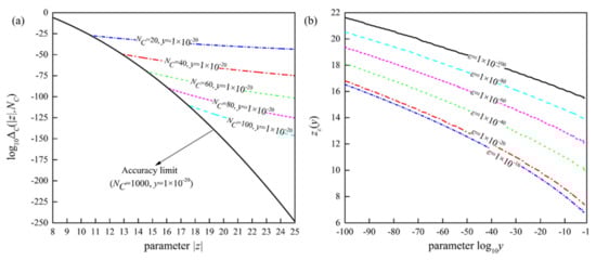
Figure 1.
(a) The approximation accuracy of Equation (23) with y = 1 × 10⁻²⁰ at different NC and (b) the efficient computing boundary zε(y) with different selected accuracy.
As we can see from Figure 1a, the relative errors at |z| = 8 are still greater than 1 × 10⁻⁶, even if NC is increased to 1000. Fortunately, the approximation accuracy of Equation (23) with y = 1 × 10⁻²⁰ increases significantly with increasing |z|, i.e., only the first 100 terms need to be taken, and the truncation of the LCF can reach the approximation accuracy of 10−100 when |z|> 16.8. Therefore, it is important to determine the efficient computing boundary of the LCF approximations, especially when y is small. The numerical calculation results illustrate that if it is desired to achieve the selected precision ε efficiently, the absolute value of argument z needs to be greater than a certain boundary zε(y) which is determined by y and ε together and can be written as follow
Figure 1b shows the zε(y) curves with selected accuracy of ε = 10−16, 10−20, 10−40, 10−60, 10−80 and 10−100, respectively, and the efficient computing boundary in the domain y ≤ 0.1 can be approximately calculated with the following formulas in Table 1. Thus, in order to improve the calculation efficiency, we use the following scheme to calculate the Voigt/complex error function with small imaginary argument:

Table 1.
Approximation formulas for zε(y) (y ≤ 0.1).
In addition, Figure 1b demonstrates that when only the calculation of the complex error function in the domain of 10−100 ≤ y ≤ 0.1 is considered, and the selected accuracy ε is no less than 10−100, the following simplified version of calculation scheme can be adopted:
3.2. Parameters Optimization
In general, the accuracy of the evaluation scheme (26) or (27) will be improved with the increase in parameters N, ND and NC. The numerical calculations, as seen in Figure 2a, show that the significant number of Dawson’s integral calculated by Equation (15) increases linearly with increasing ND, which indicates that the Dawson’s integral can efficiently perform arbitrary precision calculations. Moreover, we note that the evaluation scheme (26) or (27) has a limit accuracy related to y, even if the error caused by Dawson’s integral is ignored (see Figure 2b). Taking y = 10−4 as an example, the significant number of the Voigt/complex error function increases linearly with increasing N when N is less than 12. In contrast, when N is greater than 12, the calculation efficiency is significantly reduced. Numerical calculations suggest that greater N, ND and NC are unnecessary in some cases, we may select the optimal parameters to minimize the number of terms in the evaluation scheme (26) or (27) in order to gain computational acceleration. In this work, the optimal parameters under different accuracy levels ∆=1 × 10−100 and ∆=1 × 10⁻¹⁶ of the evaluation scheme (27) are shown in Table 2 and Table 3, respectively.
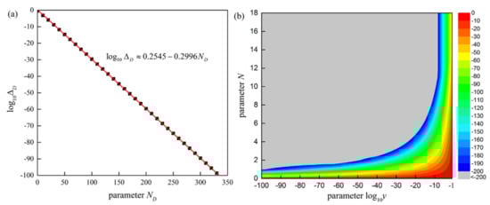
Figure 2.
(a) The maximum relative error ΔD of Dawson’s integral calculated by Equation (15) in the domain 0 ≤ x < 22 under different ND and (b) the maximum relative error Δw of Voigt/complex error function calculated by Equation (27) in the domain |x + iy| < 22 and 10−100 ≤ y ≤ 0.1 under different N and y with the error caused by the Dawson’s integral is ignored (ND = 1000).
Table 2.
The optimal parameters N, ND, and NC with accuracy levels ∆ = 1 × 10−100.
Table 3.
The optimal parameters N, ND, and NC with accuracy levels ∆ = 1 × 10⁻¹⁶.
4. Results and Discussion
4.1. Error Analysis in Multi-Precision Arithmetic
Table 1 shows that the accuracy of evaluation scheme (27) can reach 1.9055 × 10−44 when 1 × 10−100 ≤ y ≤ 0.1, and the limit accuracy is better than 1 × 10−100 when 1 × 10−100 ≤ y < 1.5849 × 10⁻⁴, which indicates that this evaluation scheme can provide highly accurate values of Voigt/complex error function with small imaginary argument, against which the accuracy achieved by fast algorithms maybe benchmarked. By contrast, Boyer and Lynas-Gray [20] used the multi-precision algorithm to calculate the high precision benchmark value of Voigt/complex error function with a maximum absolute error in both Re [w(z)] and Im [w(z)] of 10−100 for |z| ≤ 40. What is unfortunate is that Boyer and Lynas-Gray’s algorithm requires a high number of calculation bits (2000 bits) to reduce the cancellation and smearing errors, since the first 5000 terms of a series need to be calculated.
4.2. Error Analysis in Double-Precision Arithmetic
Since double-precision floating-point arithmetic is commonly used in many science computing and engineering applications, the error analysis and run-time tests of evaluation scheme (26) in double-precision arithmetic is needed. In order to quantify the accuracy of evaluation scheme (26), it is convenient to define the relative error of Re [w(z)] and Im [w(z)] as
Since the significant figure of double-precision calculation is 16 bits, the efficient computing boundary for ε = 10−16 in Table 1 is selected to distinguish the internal and external calculation domain (see Figure 3a). The parameters N and ND in the internal calculation domain are shown in Table 3 and the parameter NC for truncation of the Laplace continued fraction in the external calculation domain is shown in Figure 3b.
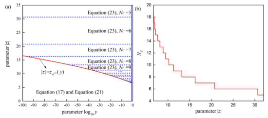
Figure 3.
(a) The evaluation scheme for Voigt/complex error function in double-precision arithmetic and (b) the parameter NC for truncation of the Laplace continued fraction in the external calculation domain.
Figure 4 shows log10∆Re for the real part of the complex error function computed over the domain 0 ≤ x ≤40,000 ∩ 10−100 ≤ y ≤ 0.1. As we can see from this figure, the evaluation scheme (26) provides accuracy better than 10−15 (green color) over the most of this domain. Although accuracy deteriorates in the neighborhood of the efficient computing boundary (see Figure 4a), it remains better than 10−13 (red color).
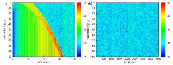
Figure 4.
The logarithm of the relative error log10∆Re for the real part of the evaluation scheme (26) over the domain (a) 0 ≤ x ≤20 ∩ 10−100 ≤ y ≤ 0.1 and (b) 20 ≤ x ≤40,000 ∩ 10−100 ≤ y ≤ 0.1, respectively.
Figure 5 illustrates log10∆Im for the imaginary part of the complex error function also computed over the domain 0 ≤ x ≤40,000 ∩ 10−100 ≤ y ≤ 0.1. As we can see from this figure, the evaluation scheme (26) provides accuracy better than 10−16 (blue color) over the most domain. Unlike the approximation for the real part, the evaluation scheme (26), also highly accurate in the neighborhood of the efficient computing boundary and the computational test, reveals that the worst accuracy is better than 10−15 (green color). One can see that the accuracy of the imaginary part is at least one order of magnitude better than the real part, which can be explained from the fact that Equation (21) is derived from Equation (17) and derivative operation enlarges calculation error.
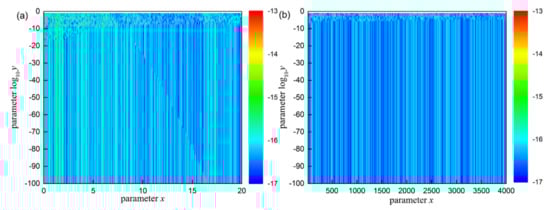
Figure 5.
The logarithm of the relative error log10∆Im for the imaginary part of the evaluation scheme (26) over the domain (a) 0 ≤ x ≤20 ∩ 10−100 ≤ y ≤ 0.1 and (b) 20 ≤ x ≤ 40,000 ∩ 10−100 ≤ y ≤ 0.1, respectively.
In Figure 6a, we compare the maximum relative error eRe(y) = max{ΔRe(x+iy) | 0 ≤ x ≤ 4000} as a function of y for the real part of the complex error function. Obviously, the calculation accuracy of “fexp” algorithm deteriorates further with decreasing y and the maximum relative error even reaches 100% when y < 10−14. The calculation accuracy of “voigtf” algorithm is better than 10−9 when y > 10−5, however, similar to “fexp” algorithm, the calculation error increases rapidly with the decrease in y when y < 10−5. When y > 10−12, “fadsamp” algorithm can achieve 10−13 calculation accuracy, however, when y < 10−12, the accuracy of this algorithm also fails. It can be seen that these algorithms have their own advantages and disadvantages; it has the benefit of a specific scope, but also needs further improvement. The common point of these algorithms is that they are not suitable for the high precision evaluation of the real part of the complex error function with small imaginary argument. Compared with to the “fexp”, “voigtf” and “fadsamp” algorithms, our new algorithm, based on evaluation scheme (26), has been significantly improved. The calculation error of the proposed algorithm in this work increases slightly with the decrease in y and the maximum relative error eRe(y) in the domain 10−100 ≤ y ≤ 0.1 is better than 2.93 × 10⁻¹³.
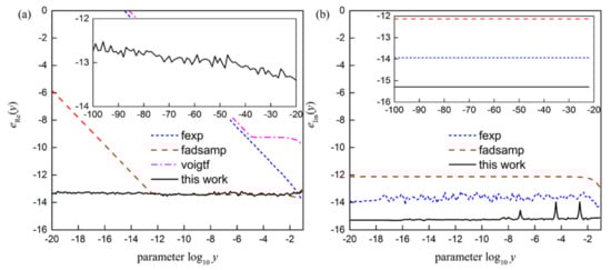
Figure 6.
The maximum relative error for the (a) real part and (b) imaginary part of complex error function.
In Figure 6b we compare the maximum relative error eIm(y) = max{ΔIm(x+iy) | 0 ≤ x ≤ 4000} as a function of y for the imaginary part of the complex error function. Fortunately, the “fexp” algorithm and “fadsamp” algorithm, as well as the proposed algorithm in this work, can achieve high-precision calculation for the imaginary part of the complex error function. Compared with the existing algorithms, the proposed algorithm has higher accuracy and the average value of the maximum relative error eIm(y) in the domain 10−100 ≤ y ≤ 0.1 is 4.91 × 10⁻¹⁶.
4.3. Preliminary Run-Time Tests with MATLAB
To obtain a first impression about the performance of the various approximations, we have used MATLAB’s built-in function “tic/toc” to evaluate the calculation speed of these algorithms. Figure 7 summarizes the results of these numerical experiments. A computational test reveals that with 1 million random numbers in different y within the internal domain |z| < 22, our algorithm is faster than “fexp” and “fadsamp” by a factor of 1.91 and 2.21, respectively (the average computing time of these algorithms is 0.33 s, 0.63 s and 0.73 s, respectively) and the “voigtf” algorithm (0.22 s) is the fastest. In the external domain 22 ≤ |z| ≤ 4000, the proposed algorithm has the highest computational efficiency, and the calculation speed is faster than “fexp”, “fadsamp” and “voigtf” algorithm by a factor of 1.44, 1.44 and 1.22, respectively (the average computing time of these algorithms is 0.18 s, 0.26 s, 0.26 s and 0.22 s, respectively). The preliminary run-time tests show that our algorithm, is as fast as those reported in recent publications.
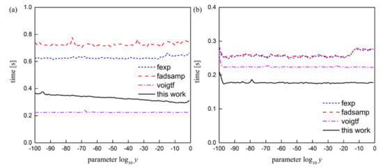
Figure 7.
Execution time (s) per algorithm evaluation with 1 million random numbers in different y within the (a) internal domain |z| < 22 and (b) external domain 22 ≤ |z| ≤ 4000, respectively. The tests have been performed on a typical desktop computer Intel(R) Quad CPU with RAM 8.00 GB. (Since the “voigtf” algorithm can only calculate the real part of the complex error function, the calculation time is doubled here to compare the calculation speed with other algorithms).
5. Conclusions
In this work we present an efficient approximation for the Voigt/complex error function that can be used for computation at small y ≤ 0.1. Error analysis and run-time tests in double-precision arithmetic reveal that in the real and imaginary parts of the proposed algorithm provide an average accuracy exceeding 10−15 and 10−16, respectively, and the calculation speed is as fast as that of reported in recent publications. Since the evaluation scheme (26) or (27) is a general expression, the desired accuracy can be easily achieved by choosing reasonable parameters. In particular, the optimal parameters under different accuracy levels ∆ = 1 × 10−100 and ∆ = 1 × 10⁻¹⁶ of evaluation scheme (27) are shown in Table 2 and Table 3, respectively, in order to gain computational acceleration. An optimized MATLAB code base on this work can be downloaded from the MATLAB Central website: https://www.mathworks.com/matlabcentral/fileexchange/75134-computing-of-voigt-complex-error-function-with-small-y (accessed on 7 January 2022).
Author Contributions
Conceptualization, Y.W.; methodology, Y.W.; MATLAB code, Y.W., B.W., R.Z., Q.L. and M.D.; validation, Y.W. and B.W.; formal analysis, Y.W.; investigation, Y.W. and B.Z.; writing—original draft preparation, Y.W.; writing—review and editing, B.Z.; visualization, Y.W., B.W., R.Z., Q.L. and M.D.; supervision, B.Z.; funding acquisition, B.Z. All authors have read and agreed to the published version of the manuscript.
Funding
This research was funded by National Key Research and Development Program of China, grant number 2017YFB0603204.
Institutional Review Board Statement
Not applicable.
Informed Consent Statement
Not applicable.
Data Availability Statement
Not applicable.
Conflicts of Interest
The authors declare no conflict of interest.
Appendix A
The 0-order and 2-order partial derivatives of L(x, y) with respect to y are expressed in terms of the Dawson’s integral D(x) of real argument x as follows:
We note that the even-order partial derivatives of L(x, y) with respect to y satisfies the following recurrence relation:
Thus Equations (9)–(14) can be easily derived from the above equation. It should be noted that the coefficients pn/2,k have the following simple expression:
However, we did not find a simple expression for the coefficients qn/2,k. Instead, the coefficients qn/2,k (N ≤ 7) is given as shown in the following Table A1 according to the recurrence relation.
Table A1.
The coefficients qn/2,k (N ≤ 7).
Table A1.
The coefficients qn/2,k (N ≤ 7).
| k = 0 | k = 1 | k = 2 | k = 3 | k = 4 | k = 5 | k = 6 | |
|---|---|---|---|---|---|---|---|
| n/2 = 0 | 0 | 0 | 0 | 0 | 0 | 0 | 0 |
| n/2 = 1 | 4 | 0 | 0 | 0 | 0 | 0 | 0 |
| n/2 = 2 | 40 | −16 | 0 | 0 | 0 | 0 | 0 |
| n/2 = 3 | 528 | −448 | 64 | 0 | 0 | 0 | 0 |
| n/2 = 4 | 8928 | −11,840 | 3456 | −256 | 0 | 0 | 0 |
| n/2 = 5 | 185,280 | −337,920 | 150,528 | −22,528 | 1024 | 0 | 0 |
| n/2 = 6 | 4,567,680 | −10,671,360 | 6,429,696 | −1,456,128 | 133,120 | −4096 | 0 |
| n/2 = 7 | 130,556,160 | −373,416,960 | 284,691,456 | −86,630,400 | 11,939,840 | −737,280 | 16,384 |
References
- Mohankumar, N.; Sen, S. On the very accurate evaluation of the Voigt functions. J. Quant. Spectrosc. Radiat. Transf. 2018, 224, 192–196. [Google Scholar] [CrossRef]
- Armstrong, B. Spectrum line profiles: The Voigt function. J. Quant. Spectrosc. Radiat. Transf. 1967, 7, 61–88. [Google Scholar] [CrossRef]
- Pagnini, G.; Mainardi, F. Evolution equations for the probabilistic generalization of the Voigt profile function. J. Comput. Appl. Math. 2010, 233, 1590–1595. [Google Scholar] [CrossRef]
- Li, J.; Yu, Z.; Du, Z.; Ji, Y.; Liu, C. Standoff Chemical Detection Using Laser Absorption Spectroscopy: A Review. Remote. Sens. 2020, 12, 2771. [Google Scholar] [CrossRef]
- Quine, B.M.; Drummond, J.R. GENSPECT: A line-by-line code with selectable interpolation error tolerance. J. Quant. Spectrosc. Radiat. Transf. 2002, 74, 147–165. [Google Scholar] [CrossRef]
- Siddiqui, R.; Jagpal, R.K.; Abrarov, S.M.; Quine, B.M. Efficient Application of the Radiance Enhancement Method for Detection of the Forest Fires Due to Combustion-Originated Reflectance. J. Environ. Prot. 2021, 12, 717–733. [Google Scholar] [CrossRef]
- Siddiqui, R.; Jagpal, R.K.; Abrarov, S.M.; Quine, B.M. Radiance enhancement and shortwave upwelling radiative flux methods for efficient detection of cloud scenes. Int. J. Space Sci. Eng. 2020, 6, 1–27. [Google Scholar] [CrossRef]
- Wang, Y.; Zhou, B.; Liu, C. Calibration-free wavelength modulation spectroscopy based on even-order harmonics. Opt. Express 2021, 29, 26618. [Google Scholar] [CrossRef]
- Wang, Y.; Zhou, B.; Liu, C. Sensitivity and Accuracy Enhanced Wavelength Modulation Spectroscopy Based on PSD Analysis. IEEE Photon.-Technol. Lett. 2021, 33, 1487–1490. [Google Scholar] [CrossRef]
- Enemali, G.; Zhang, R.; McCann, H.; Liu, C. Cost-Effective Quasi-Parallel Sensing Instrumentation for Industrial Chemical Species Tomography. IEEE Trans. Ind. Electron. 2021, 69, 2107–2116. [Google Scholar] [CrossRef]
- Khan, S.; Agrawal, B.; Pathan, M. Some connections between generalized Voigt functions with the different parameters. Appl. Math. Comput. 2006, 181, 57–64. [Google Scholar] [CrossRef]
- Bao, Y.; Zhang, R.; Enemali, G.; Cao, Z.; Zhou, B.; McCann, H.; Liu, C. Relative Entropy Regularized TDLAS Tomography for Robust Temperature Imaging. IEEE Trans. Instrum. Meas. 2021, 70, 1–9. [Google Scholar] [CrossRef]
- Wang, Y.; Zhou, B.; Zhao, R.; Wang, B.; Liu, Q.; Dai, M. Super-Accuracy Calculation for the Half Width of a Voigt Profile. Mathematics 2022, 10, 210. [Google Scholar] [CrossRef]
- Li, R.; Li, F.; Lin, X.; Yu, X. Error Analysis of Integrated Absorbance for TDLAS in a Nonuniform Flow Field. Appl. Sci. 2021, 11, 10936. [Google Scholar] [CrossRef]
- Wang, Z.; Fu, P.; Chao, X. Laser Absorption Sensing Systems: Challenges, Modeling, and Design Optimization. Appl. Sci. 2019, 9, 2723. [Google Scholar] [CrossRef]
- Ma, L.; Duan, K.; Cheong, K.P.; Yuan, C.; Ren, W. Multispectral infrared absorption spectroscopy for quantitative temperature measurements in axisymmetric laminar premixed sooting flames. Case Stud. Therm. Eng. 2021, 28, 101575. [Google Scholar] [CrossRef]
- Poppe, G.P.M.; Wijers, C.M.J. Algorithm 680: Evaluation of the complex error function. ACM Trans. Math. Softw. 1990, 16, 47. [Google Scholar] [CrossRef]
- Poppe, G.P.M.; Wijers, C.M.J. More efficient computation of the complex error function. ACM Trans. Math. Softw. 1990, 16, 38–46. [Google Scholar] [CrossRef]
- Zaghloul, M.R.; Ali, A.N. Algorithm 916: Computing the Faddeyeva and Voigt Functions. ACM Trans. Math. Softw. 2011, 38, 1–22. [Google Scholar] [CrossRef]
- Boyer, W.; Lynas-Gray, A.E. Evaluation of the Voigt function to arbitrary precision. Mon. Not. R. Astron. Soc. 2014, 444, 2555–2560. [Google Scholar] [CrossRef]
- Molin, P. Multi-Precision Computation of the Complex Error Function. 2011. Available online: https://hal.archives-ouvertes.fr/hal-00580855 (accessed on 26 December 2021).
- Bailey, J.; Kedziora-Chudczer, L. Modelling the spectra of planets, brown dwarfs and stars using vstar. Mon. Not. R. Astron. Soc. 2011, 419, 1913–1929. [Google Scholar] [CrossRef]
- Liu, Y.; Lin, J.; Huang, G.; Guo, Y.; Duan, C. Simple empirical analytical approximation to the Voigt profile. J. Opt. Soc. Am. B 2001, 18, 666–672. [Google Scholar] [CrossRef]
- Di Rocco, H.; Cruzado, A. The Voigt Profile as a Sum of a Gaussian and a Lorentzian Functions, when the Weight Coefficient Depends Only on the Widths Ratio. Acta Phys. Pol. A 2012, 122, 666–669. [Google Scholar] [CrossRef]
- Ida, T.; Ando, M.; Toraya, H. Extended pseudo-Voigt function for approximating the Voigt profile. J. Appl. Crystallogr. 2000, 33, 1311–1316. [Google Scholar] [CrossRef]
- Schreier, F. The Voigt and complex error function: Humlicek’s rational approximation generalized. Mon. Not. R. Astron. Soc. 2018, 479, 3068–3075. [Google Scholar] [CrossRef]
- Humlíček, J. An efficient method for evaluation of the complex probability function: The Voigt function and its derivatives. J. Quant. Spectrosc. Radiat. Transf. 1979, 21, 309–313. [Google Scholar] [CrossRef]
- Humlíček, J. Optimized computation of the voigt and complex probability functions. J. Quant. Spectrosc. Radiat. Transf. 1982, 27, 437–444. [Google Scholar] [CrossRef]
- Imai, K.; Suzuki, M.; Takahashi, C. Evaluation of Voigt algorithms for the ISS/JEM/SMILES L2 data processing system. Adv. Space Res. 2009, 45, 669–675. [Google Scholar] [CrossRef]
- Tennyson, J.; Bernath, P.F.; Campargue, A.; Császár, A.G.; Daumont, L.; Gamache, R.R.; Hodges, J.T.; Lisak, D.; Naumenko, O.V.; Rothman, L.; et al. Recommended isolated-line profile for representing high-resolution spectroscopic transitions (IUPAC Technical Report). Pure Appl. Chem. 2014, 86, 1931–1943. [Google Scholar] [CrossRef]
- Tran, H.; Ngo, N.; Hartmann, J.-M. Efficient computation of some speed-dependent isolated line profiles. J. Quant. Spectrosc. Radiat. Transf. 2013, 129, 199–203. [Google Scholar] [CrossRef]
- Abrarov, S.; Quine, B.; Jagpal, R. High-accuracy approximation of the complex probability function by Fourier expansion of exponential multiplier. Comput. Phys. Commun. 2010, 181, 876–882. [Google Scholar] [CrossRef]
- Abrarov, S.; Quine, B.; Jagpal, R. Rapidly convergent series for high-accuracy calculation of the Voigt function. J. Quant. Spectrosc. Radiat. Transf. 2010, 111, 372–375. [Google Scholar] [CrossRef]
- Abrarov, S.M.; Quine, B.M. A rational approximation for efficient computation of the Voigt function in quantitative spectroscopy. J. Math. Res. 2015, 7, 163–174. [Google Scholar] [CrossRef]
- Abrarov, S.M.; Quine, B.M.; Jagpal, R.K. A sampling-based approximation of the complex error function and its implementation without poles. Appl. Numer. Math. 2018, 129, 181–191. [Google Scholar] [CrossRef]
- Abrarov, S.M.; Quine, B.M. Accurate Approximations for the Complex Error Function with Small Imaginary Argument. J. Math. Res. 2015, 7, 44–53. [Google Scholar] [CrossRef]
- Rutkowski, L.; Maslowski, P.; Johansson, A.C.; Khodabakhsh, A.; Foltynowicz, A. Optical frequency comb Fourier transform spectroscopy with sub-nominal resolution and precision beyond the Voigt profile. J. Quant. Spectrosc. Radiat. Transf. 2018, 204, 63–73. [Google Scholar] [CrossRef]
- Gradshteĭn, I.S.; Ryzhik, I.M. Table of Integrals, Series, and Products; Academic Press: Cambridge, MA, USA, 2014. [Google Scholar]
- McCabe, J.H. A continued fraction expansion, with a truncation error estimate, for Dawson’s integral. Math. Comput. 1974, 28, 811–816. [Google Scholar] [CrossRef]
- Rybicki, G.B. Dawson’s integral and the sampling theorem. Comput. Phys. 1989, 3, 85–87. [Google Scholar] [CrossRef]
- Boyd, J. Evaluating of Dawson’s Integral by solving its differential equation using orthogonal rational Chebyshev functions. Appl. Math. Comput. 2008, 204, 914–919. [Google Scholar] [CrossRef]
- Abrarov, S.M.; Quine, B.M. A rational approximation of the Dawson’s integral for efficient computation of the complex error function. Appl. Math. Comput. 2018, 321, 526–543. [Google Scholar] [CrossRef]


Publisher’s Note: MDPI stays neutral with regard to jurisdictional claims in published maps and institutional affiliations. |
© 2022 by the authors. Licensee MDPI, Basel, Switzerland. This article is an open access article distributed under the terms and conditions of the Creative Commons Attribution (CC BY) license (https://creativecommons.org/licenses/by/4.0/).