Abstract
A simple approximation scheme to describe the half width of the Voigt profile as a function of the relative contributions of Gaussian and Lorentzian broadening is presented. The proposed approximation scheme is highly accurate and provides an accuracy better than 10−17 for arbitrary αL/αG ratios. In particular, the accuracy reaches an astonishing 10−34 (quadruple precision) in the domain 0 ≤ αL/αG ≤ 0.2371 ∪ αL/αG ≥ 33.8786.
1. Introduction
The Voigt profile is widely used in optics, laser physics, plasma, astrophysics and spectroscopy [1,2,3,4,5,6]. By the convolution of both the Lorentzian and Gaussian profiles, the Voigt profile blends the physical characteristics of both profiles. Whereas the Lorentzian is associated with lifetime effects, the Gaussian is associated with thermal and statistical effects [7,8]. Accurate calculations and approximations for the Voigt spectral quantities in terms of the Gaussian and Lorentzian admixture are essential for the quantification of the profile. In actual application, the half width at half maximum (HWHM) of the Voigt profile, αV, is important [8,9,10,11,12]. Unfortunately, there is no analytically exact expression to describe the HWHM of the Voigt profile as a function of the HWHMs of the Lorentzian and Gaussian profiles, αL and αG, respectively, and thus many approximations have been presented in the past to find simple relationships, i.e., composed of basic elementary functions only, between αV, αL and αG [13,14,15,16,17].
The approximation expression developed by Olivero and Longbothum (Equation (5) in [17]), to the best of the authors’ knowledge, is the most accurate, and its estimation error is less than 0.01%. Although this approximation is sufficient for the most practical tasks, the more accurate approximation may also be required in modern precision spectroscopy [18]. Several highly accurate codes, such as the ACM Algorithm 680 [19,20] (14 significant digits stated accuracy) and ACM Algorithm 916 [21] (20 significant digits) or arbitrary precision codes [22,23], are indispensable for evaluation of the Voigt profile, but not necessarily fast. However, in some cases, where we only focus on broadening [8,9,10,11,12,24], it is unwise to use these highly accurate codes. Therefore, a highly accurate approximate scheme specially used to evaluate the half width at half maximum of the Voigt profile is urgently needed.
In this work, we present a simple approximation scheme to describe the half width of the Voigt profile as a function of the relative contributions of Gaussian and Lorentzian broadening. The numerical calculations suggest that the proposed approximation expression can achieve super-accuracy calculation for Voigt profiles for arbitrary αL/αG ratios. The rest of the paper is organized as follows: Section 2 details the methodology and derivation of the proposed approximation scheme. Error analysis and an applicable example for Doppler-broadening thermometry (DBT) are carried out to validate the proposed approximation scheme in Section 3 and Section 4, respectively. The paper is finally summarized in Section 5.
2. Methodology and Derivation
The Voigt profile gV is the convolution of both the Lorentz profile gL and the Gaussian profile gG given by [25]
where ⊗ is the convolution functional and v is a generalized parameter for the wavenumber, frequency or photon energy. The Voigt function K(x,y), normalized to ,
has been introduced for mathematical convenience. Here, the dimensionless variables , are a measure for the distance from the peak center v0 and for the ratio of Lorentzian to Gaussian width, respectively, and z = x+ iy. At the line center x = 0, the Voigt function can be expressed as the exponentially scaled complementary error function K(0, y) = exp(y2)erfc(y). Thus, the half-width scale in units of Gaussian broadening of a Voigt profile, Γ, for a given value of y is given by the following equation:
where Γ is defined as . The variables x and y are more convenient for lines which are predominantly Gaussian while the variables X = x/y and η = 1/y are more convenient for lines which are predominantly Lorentz [26]. Thus, the half-width scale in units of Lorentzian broadening of a Voigt profile,, for a given value of η is given by the following equation:
whereis defined as = αV/αL.
Considering the Gaussian limit (y→0) and the Lorentz limit (y→∞) of Equation (1) [18]
the following two half-width limits can be easily deduced
2.1. The Half Width of Voigt Profile with Small y (0 ≤ y ≤ 0.6993)
Combining Equations (2) and (3), the following equation for the half-width scale in units of Gaussian broadening, Γ, can be obtained
Suppose that the half width Γ of a Voigt profile with small y can be expanded by the following power series
By combining Equations (8) and (9) and using the method of equating coefficients, any of the coefficients pn in Equation (9) can be determined. In this work, we have derived the recurrence equation satisfied by the expression of the (r + 1)-th coefficient pr (r ≥ 1) of each order in Equation (9) as follows
where each coefficient in the above expression can be calculated by the first r coefficients, p0, p1, …, pr−1. The derivation of Equation (10) and the definition of each coefficient can be found in Appendix A. We notice the fact that Γ = at y = 0, which indicates that the first coefficient p0 = . Therefore, the coefficient of each order in Equation (9) can be obtained immediately by solving the recurrence equation. For example, the first four coefficients are shown as follows
where constants θ1 = , θ2 = and θ3 = , respectively, and erfi(z) = −ierf(iz) is the imaginary error function. In addition, the first 31 terms with 32 significant digits are given in Table A1.
2.2. The Half Width of Voigt Profile with Large y (y ≥ 8.2507)
Numerical analysis, detailed in Appendix B, indicates that it is convenient to analyze the relationship between and η, and a simple series is given as following
In the above expression, the coefficients of odd terms are all zero, and the even terms are all rational fractions, which are conducive to high-precision calculation.
2.3. The Half Width of Voigt Profile with Middle y (0.6993 < y < 8.2507)
The global nature of the Chebyshev approximation over finite intervals [27] overcomes the range limitations resulting from the asymptotic expansions of Equations (9) and (12). Because of the best uniform approximation property of the Chebyshev polynomial, the best uniform approximation expression of the Voigt profile with middle y (0.6993 < y < 8.2507) can be obtained. Numerical analysis suggests that it is useful to introduce the non-dimensional quantities R = αV/(αL + αG) and D = (αL − αG)/(αL + αG) = ( y − )/( y + ), and the best uniform approximation expression is given as following
where (Dk, R(Dk)) are a set of N sample points without two identical points of Dk, and Dk are given as following
For computational convenience, the above mathematical expression can be reformulated into the following equivalent form
where the first 31 coefficients, uk, with 32 significant digits are given in Table A3.
2.4. Half Width Approximation Scheme for Arbitrary Voigt Profile
In summary, two asymptotic expansions, Equations (9) and (12), are given for smaller y and larger y, respectively, and a Chebyshev approximation, Equation (15), for middle y. Thus, the half-width approximation scheme, using the same variable y, for an arbitrary Voigt profile can be summarized as follows:
It is worth pointing out that when the approximation scheme Equation (16) is implemented on a double precision platform, the accuracy is reduced due to the rounding errors. An improvement approximation scheme for double precision platforms is as follows:
3. Error Analysis
Define the relative errors for the half width of Voigt profile in the form
where [αV]appr. is the approximate value given by Equation (16) or Equation (17) and [αV]ref. is the reference. The highly accurate reference values of the half width can be obtained by solving Equation (3) using the latest versions of MATLAB that supports the symbolic computing system with high number, i.e., 128 in this work, of significand precision.
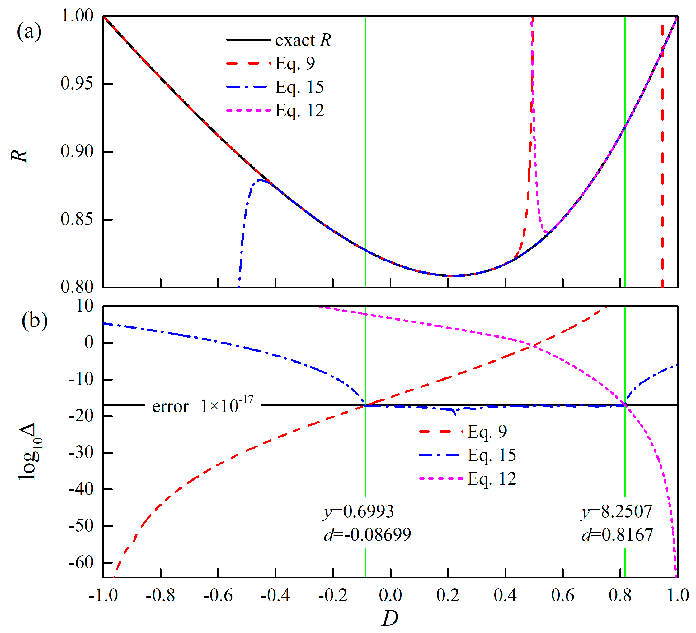
Figure 1 shows (a) the comparison of each half-width functions and (b) the logarithm of relative error for the half width of the Voigt profile, respectively, in the R, D format on a high-precision platform. As we can see, in the Gaussian dominant region, i.e., 0 ≤ y ≤ 0.6993 (−1 ≤ D ≤ −0.0870), the approximation Equation (9) is highly accurate and provides an accuracy better than 10−17. Numerical results illustrate that the calculation accuracy of Equation (9) increases significantly with the decrease of y, which indicates that this expression is more suitable for the calculation of small y. In particular, the accuracy of Equation (9) can reach the super accuracy of 10−34 (quadruple precision) in the domain 0 ≤ y ≤ 0.1974 (−1 ≤ D ≤ −0.6167). Similarly, in the Lorentz dominant region, i.e., y ≥ 8.2507 (0.8167 ≤ D ≤ 1), the approximation Equation (12) is highly accurate and provides an accuracy better than 10−17.
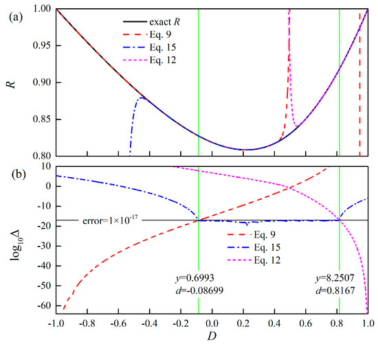
Figure 1.
(a) The comparison of each half-width function and (b) the logarithm of relative error for the half width of the Voigt profile, respectively, in the R, D format.
Numerical results show that the calculation accuracy of Equation (12) increases significantly with the increase of y, which indicates that this expression is more suitable for the calculation of large y. In particular, the accuracy of Equation (12) can reach the super- accuracy of 10−34 in the domain y ≥ 28.2058 (0.9427 ≤ D ≤ 1). The Voigt width approximation is particularly important in the middle region, i.e., 0.6993 < y < 8.2507 (−0.0870 < D< 0.8167), in which the width of the Gaussian profile is comparable to the width of the Lorentzian profile. Numerical results show that the approximation Equation (15) based on Chebyshev approximation with 30 degree is highly accurate and provides an accuracy better than 10−17 in the middle region. In summary, the approximation scheme Equation (16) is highly accurate and provides an accuracy better than 10−17 for arbitrary αL/αG ratios, which indicates that the calculation error can be ignored for the general double-precision calculation platform (16 bits).
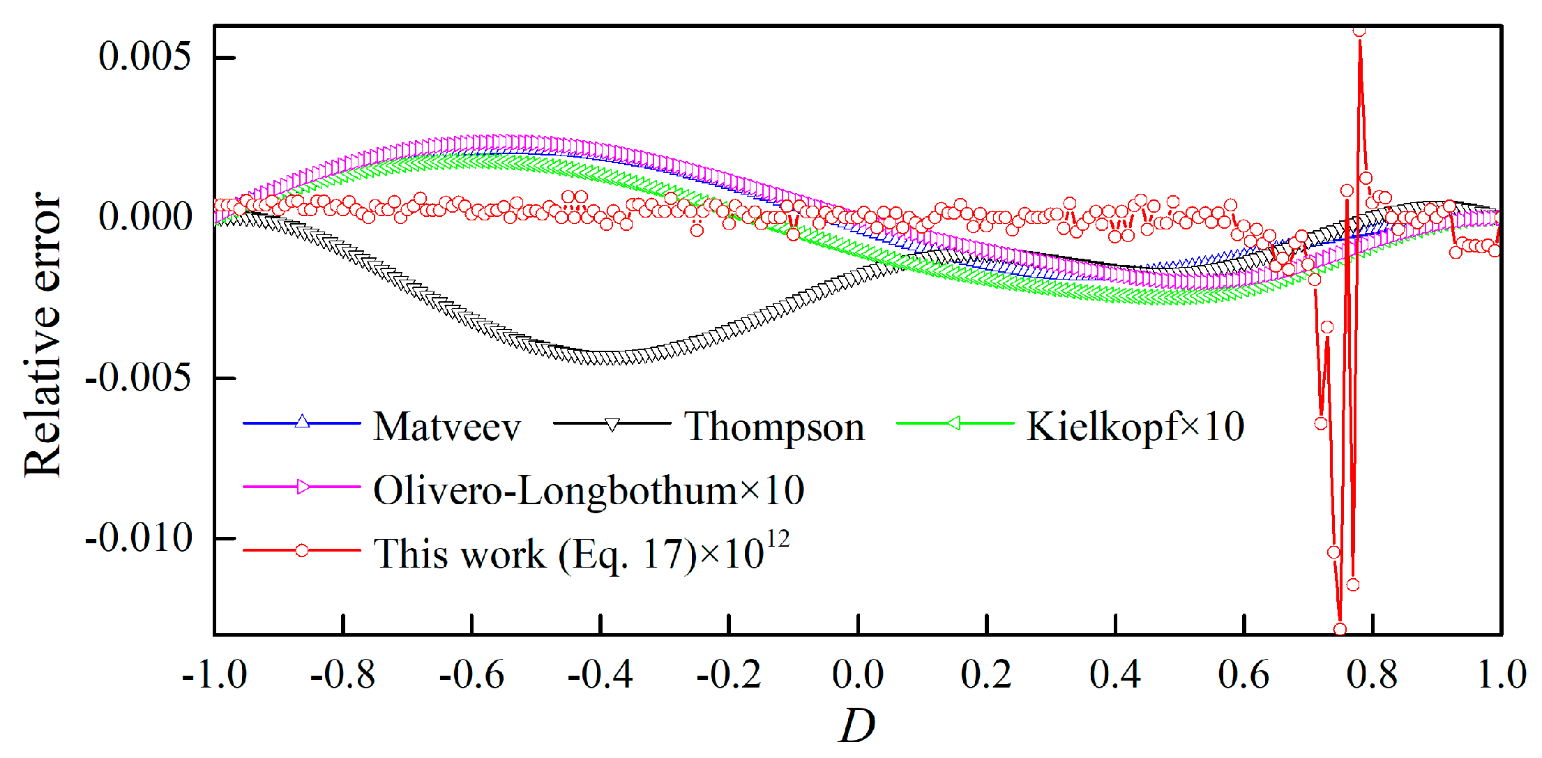
Furthermore, the accuracy of the proposed approximation scheme is compared with several commonly used approximation expressions [14,15,16,17] on a double precision platform. These approximate expressions are summarized in Table 1. The relative errors of different approximation schemes on a double precision platform are shown in Figure 2. The maximum relative errors of Matveev, Thompson, Kielkopf and Olivero–Longbothum are 2.14 × 10⁻², 4.32 × 10⁻², 2.48 × 10⁻⁴ and 2.37 × 10⁻⁴, respectively. As a comparison, the calculation accuracy of the proposed approximation scheme is significantly improved, and its maximum relative error is 1.28 × 10⁻¹⁴.

Table 1.
Empirical fit to the Voigt half width.
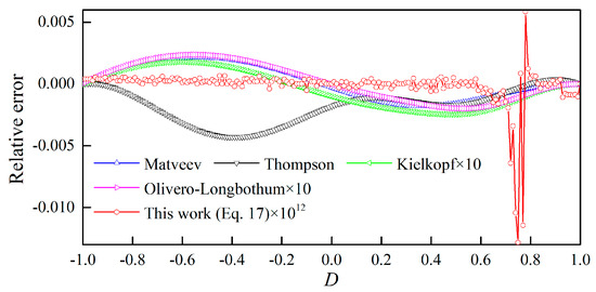
Figure 2.
The relative errors of different approximation schemes on a double precision platform.
4. An Applicable Example: Doppler-Broadening Thermometry (DBT)
To evaluate the superiority of the proposed approximation scheme in terms of computational accuracy, a numerical simulation experiment of Doppler-broadening thermometry (DBT) using carbon dioxide (CO2) transitions is presented in this section. The Pe(12) line of the 30012 ← 00001 band of CO2, centered at 6337.990338 cm−1 with strength of 1.526 × 10⁻²³ cm/molecule [28], is used in this simulation. DBT is potentially an accurate and practical approach for thermodynamic temperature measurement [12,24]. DBT consists of retrieving the half width of Gaussian profile, αG, from the highly accurate observation of the shape of a given atomic or molecular line, in a laser-based absorption-spectroscopy experiment under a linear regime of radiation-matter interaction [12]. Once αG is known, the thermodynamic temperature can be calculated as
where v0 = 6337.990338 cm−1 is the central frequency, kB = 1.38064852 × 10⁻²³ J/K the Boltzmann constant, c = 2.99792485 × 10⁸ m/s the speed of light and m = 7.308032313279367 × 10⁻²⁶ kg the mass of CO2.
In general, the measured Voigt profile is deconvoluted to extract the Gaussian profile component, and then, the thermodynamic temperature is obtained by Equation (19). In this work, a simple deconvolution method based on the maximum and half width of the Voigt profile is used [29]. This method can easily calculate the half width of a Gaussian profile by solving the following non-linear system of equations
where gV,max is the measured maximum of the Voigt profile and F(αL,αG) is some formula used for the half-width approximation. In this section, we only examine the numerical simulation results of the proposed approximation scheme Equation (17) and the Olivero-Longbothum approximation.
The simulated Voigt profiles of Pe(12) line of CO2 at different pressures are shown in Figure 3. Obviously, the half width of the Voigt profile increases with higher pressure. This is because the Lorentzian broadening caused by molecular collisions becomes more and more significant as the pressure increases. Furthermore, the absolute deviations of DBT temperature calculations using different half-width approximations in the pressure range of 1 Pa to 2000 Pa are shown in Figure 4. Numerical simulation results demonstrate that the absolute temperature deviation is always less than 1.19 × 10⁻¹² K while the proposed approximation scheme Equation (17) is used for DBT temperature calculations. In contrast, the absolute temperature deviation becomes larger rapidly as the pressure increases for the Olivero-Longbothum approximation. The simulation experiments in this section reveal that a much more accurate half-width approximation scheme for an arbitrary Voigt profile is necessary when we expect to achieve high-accuracy temperature measurements at the mK level [12] using the Doppler-broadening thermometry method.
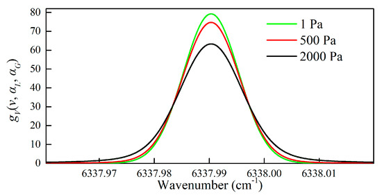
Figure 3.
The simulated Voigt profile of Pe(12) line of CO2 at different pressures (CO2 concentration is 1000 ppm, temperature is 300 K).
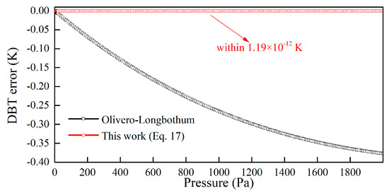
Figure 4.
The absolute deviations of DBT temperature calculations using different half-width approximations.
5. Conclusions
A simple approximation scheme to describe the half width of the Voigt profile as a function of the relative contributions of Gaussian and Lorentzian broadening is presented in this work. The numerical calculations suggest that the proposed approximation scheme can achieve super-accuracy (better than 10−17) calculation for Voigt profiles for arbitrary αL/αG ratios. In particular, the accuracy reaches an astonishing 10−34 in the domain 0 ≤ y ≤ 0.1974∪y ≥ 28.2058(0 ≤ αL/αG ≤ 0.2371∪αL/αG ≥ 33.8786). Furthermore, the coefficients in Equation (12) are all simple rational fractions, and the law behind this expression is also an interesting mathematical problem worth exploring. To evaluate the superiority of the proposed approximation scheme in terms of computational accuracy, a numerical simulation experiments of Doppler-broadening thermometry using carbon dioxide transitions is presented in this work. In addition, three simplified MATLAB codes can be found at the MATLAB Central website: https://www.mathworks.cn/matlabcentral/fileexchange/95283-highly-accurate-width-of-the-voigt-profile (accessed on 26 December 2021).
Author Contributions
Conceptualization, Y.W.; methodology, Y.W.; MATLAB code, Y.W., R.Z., B.W., Q.L. and M.D.; validation, Y.W. and R.Z.; formal analysis, Y.W.; investigation, Y.W. and B.Z.; writing—original draft preparation, Y.W.; writing—review and editing, B.Z.; visualization, Y.W., B.W., R.Z., Q.L. and M.D.; supervision, B.Z.; funding acquisition, B.Z. All authors have read and agreed to the published version of the manuscript.
Funding
This research was funded by National Key Research and Development Program of China, grant number 2017YFB0603204.
Institutional Review Board Statement
Not applicable.
Informed Consent Statement
Not applicable.
Data Availability Statement
Not applicable.
Conflicts of Interest
The authors declare no conflict of interest.
Appendix A
In this part, we derive the expression of the (r + 1)-th coefficient pr from the first r coefficients p0, p1, …, pr−1 (r >= 1) using the series analysis method.
- Step 1: Series expansion for the factors in Equation (5) at y = 0
(1) Series expansion for
The exponential function can be expanded into the following series at y = 0:
where the coefficients an are defined as:
where (.)n is the Pochhammer symbol. According to the multinomial theorem, Equation (A3) can be rewritten as follows, in ascending order of the degree of y:
where the coefficients dk are defined as:
where the coefficients αn,k,j are defined as:
(2) Series expansion for
In the same way, the exponential function can be expanded into the following series at y = 0:
where the coefficients fk are defined as:
where the coefficients bn are defined as:
(3) Series expansion for sin(2Γy)
In the same way, the sine function sin(2Γy) can be expanded into the following series at y = 0:
where the coefficients gm are defined as:
where the coefficients βn,k,j are defined as:
(4) Series expansion for cos(2Γy)
In the same way, the cosine function cos(2Γy) can be expanded into the following series at y = 0:
where the coefficients hm are defined as:
(5) Series expansion for erfi(Γ)
In the same way, the imaginary error function erfi(Γ) can be expanded into the following series at y = 0:
where the coefficients en are defined as:
(6) Series expansion for erfc(y − iΓ)
The complementary error function erfc(y − iΓ) can be expanded into the following series at y = 0:
and the third term in the above formula can be reduced to the following formula:
where the coefficients cn are defined as:
where the coefficients γn,k,j are defined as:
Considering the expansion series of Equations (A2) and (A18), the third term in Equation (A17) can be reduced to the following formula:
By substituting Equations (A15) and (A21) into Equation (A17), the expressions of real part and imaginary part of the complementary error function erfc(y − iΓ) can be expanded into the following series:
respectively, where the coefficients lk and qk are defined as:
(7) Series expansion for erfc(y)
The error function erfc(y) can be expanded into the following series at y = 0:
where the coefficients sn are defined as:
- Step 2: Calculate pr by the method of comparing coefficients
By substituting Equations (A7), (A10), (A13), (A22) and (A25) into Equation (8), the following expression is obtained:
Therefore, a mathematical expression to determine the (r + 1)-th coefficient pr is obtained by using the method of comparing coefficients:
The recurrence equation satisfied by the expression of the (r + 1)-th coefficient pr can be obtained by simplifying the above expression:
Considering the initial value p0 = , arbitrary term coefficients pn can be calculated by using Equation (A29), and the first 31 coefficients pn with 32 significant digits are given in Table A1.
Table A1.
The first 31 coefficients pn in Equation (9) with 32 significant digits.
Table A1.
The first 31 coefficients pn in Equation (9) with 32 significant digits.
| n | pn | n | pn |
|---|---|---|---|
| 0 | 0.8325546111576977563531646448952 | 16 | 2.5308903977393059634088084205148 × 10⁻⁸ |
| 1 | 0.53254711842961210323020845059416 | 17 | −3.3104307709547517055285672959576 × 10⁻⁸ |
| 2 | 0.13603423870145348659601346974136 | 18 | −1.1821070040002130133075915099552 × 10⁻⁸ |
| 3 | −6.3839925995348583105863651935208 × 10⁻³ | 19 | 5.0020607880755762331999675884955 × 10⁻⁹ |
| 4 | −7.5882994178697868047017954181619 × 10⁻³ | 20 | 3.2040951850692659104678394048668 × 10⁻⁹ |
| 5 | 7.5685451134845100193553849814044 × 10⁻⁴ | 21 | −4.9276721508012916216290609360574 × 10⁻¹⁰ |
| 6 | 6.4174309726033170181322853645455 × 10⁻⁴ | 22 | −7.1352246104725448681836423474852 × 10⁻¹⁰ |
| 7 | −1.0278614365257442345642575963235 × 10⁻⁵ | 23 | −3.2407999521382539130974667691197 × 10⁻¹¹ |
| 8 | −6.6864392638387619203117167133824 × 10⁻⁵ | 24 | 1.4010883014405512366881008147675 × 10⁻¹⁰ |
| 9 | −1.8800729899141457354675112660009 × 10⁻⁵ | 25 | 3.3772678382804066494130831543588 × 10⁻¹¹ |
| 10 | 9.3901358253570724565409358708571 × 10⁻⁶ | 26 | −2.3680267709485323621904030934022 × 10⁻¹¹ |
| 11 | 5.4149990265667553408636905696295 × 10⁻⁶ | 27 | −1.1462686830778835681784218983719 × 10⁻¹¹ |
| 12 | −1.2862976252461744893956942201673 × 10⁻⁶ | 28 | 3.0039670445166124668988923778107 × 10⁻¹² |
| 13 | −1.0759168918380548822306060203341 × 10⁻⁶ | 29 | 2.9478889620399924642669859987364 × 10⁻¹² |
| 14 | 7.8733635964790862989086501951507 × 10⁻⁸ | 30 | −9.7467645599626148566298439388065 × 10⁻¹⁴ |
| 15 | 1.9255725519174188542320412973488 × 10⁻⁷ |
Appendix B
The relationship between and η can be written in the form of Taylor series as follows:
where T0 = 1 and the coefficients Tn (n > 1) can be estimated by the following recurrence relations:
In this work, the parameter ε in the above equation is set to 1 × 10⁻²⁰ and the benchmark value of is obtained according to Equation (3) by using the latest versions of MATLAB that supports the symbolic computing system with high number of significand precision. The coefficients Tn and Tn* of the first 31 terms are given in Table A2. Numerical calculation results suggest that the Tn* value can be rewritten as the sum of a rational fraction and a fairly small remainder. Fortunately, the reduction in accuracy due to the elimination of the remainder is negligible.
Table A2.
The first 31 coefficients Tn in Equation (12).
Table A2.
The first 31 coefficients Tn in Equation (12).
| n | Tn* | Tn | n | Tn* | Tn |
|---|---|---|---|---|---|
| 0 | / | 1 | 16 | ≈−25390179/211 + 1.1 × 10⁻³⁵ | −25390179/211 |
| 1 | ≈0 + 1.5 × 10⁻²⁰ | 0 | 17 | ≈0 + 1.1 × 10⁻¹⁵ | 0 |
| 2 | ≈3/2 − 7.5 × 10−41 | 3/2 | 18 | ≈446848569/212 − 1.1 × 10⁻³⁴ | 446848569/212 |
| 3 | ≈0 − 7.5 × 10⁻²¹ | 0 | 19 | ≈0 + −1.1 × 10⁻¹⁴ | 0 |
| 4 | ≈−3/22 + 1.9 × 10−40 | −3/22 | 20 | ≈−1089694161/210 + 1.1 × 10⁻³³ | −1089694161/210 |
| 5 | ≈0 + 1.9 × 10⁻²⁰ | 0 | 21 | ≈0 + 1.1 × 10⁻¹³ | 0 |
| 6 | ≈15/23 − 7.6 × 10−40 | 15/23 | 22 | ≈46704949839/212 − 1.3 × 10⁻³² | 46704949839/212 |
| 7 | ≈0 − 7.6 × 10⁻²⁰ | 0 | 23 | ≈0 − 1.3 × 10⁻¹² | 0 |
| 8 | ≈−243/25 + 3.9 × 10−39 | −243/25 | 24 | ≈−8735832539883/216 + 1.7 × 10⁻³¹ | −8735832539883/216 |
| 9 | ≈0 + 3.9 × 10⁻¹⁹ | 0 | 25 | ≈0 + 1.7 × 10⁻¹¹ | 0 |
| 10 | ≈2493/26 − 2.3 × 10−38 | 2493/26 | 26 | ≈221377058104455/217 − 2.3 × 10⁻³⁰ | 221377058104455/217 |
| 11 | ≈0 − 2.3 × 10⁻¹⁸ | 0 | 27 | ≈0 − 2.3 × 10⁻¹⁰ | 0 |
| 12 | ≈−927/22 + 1.6 × 10−37 | −927/22 | 28 | ≈−6044700753428715/218 + 3.4 × 10⁻²⁹ | −6044700753428715/218 |
| 13 | ≈0 + 1.6 × 10⁻¹⁷ | 0 | 29 | ≈0 + 3.4 × 10⁻⁹ | 0 |
| 14 | ≈405783/28 − 1.2 × 10−36 | 405783/28 | 30 | ≈176955754371862947/219 + 3.9 × 10⁻⁸ | 176955754371862947/219 |
| 15 | ≈0 − 1.2 × 10⁻¹⁶ | 0 |
Appendix C
Table A3.
The first 31 coefficients un in Equation (15) with 32 significant digits.
Table A3.
The first 31 coefficients un in Equation (15) with 32 significant digits.
| n | un | n | un |
|---|---|---|---|
| 0 | 0.81879767981374096480451126966969 | 16 | −11.608186550060767559947858982236 |
| 1 | −0.087358831239253690600565585478191 | 17 | 98.530866614251729915080851559823 |
| 2 | 0.16111263881308988360982026625923 | 18 | −520.58001078415212154632736105054 |
| 3 | 0.10352476879958392716101379868109 | 19 | 1996.0992356052342655084175033613 |
| 4 | 0.044701941374241324794152587529398 | 20 | −5861.8655902675083091764869931816 |
| 5 | −0.0014922440275783965022042298334427 | 21 | 13508.475417035315538373423012345 |
| 6 | −0.025999766558392062049748550766996 | 22 | −24679.618517222644663493302537093 |
| 7 | −0.027433278283219905509735236616617 | 23 | 35800.136359576107078418696532107 |
| 8 | −0.012324451041403454228824532372558 | 24 | −41003.133466095685472430284467431 |
| 9 | 0.0076580003679061144826236693340858 | 25 | 36602.695793508138571786897415062 |
| 10 | 0.020609356479185309053858762785961 | 26 | −24908.669183448932665943004856528 |
| 11 | 0.019910337726501870836014131102016 | 27 | 12466.93366679248692417862886569 |
| 12 | 0.0077590409364772777791275317929576 | 28 | −4321.2090018088841034237110866818 |
| 13 | −0.047206722791611042489905888231109 | 29 | 925.71414182435000624708620108582 |
| 14 | 0.16487160565916573888004662456667 | 30 | −92.27479145146679165668461921968 |
| 15 | 0.22613547743220062910838574670492 |
References
- Irmak, H. Various results for series expansions of the error functions with the complex variable and some of their implications. Turk. J. Math. 2020, 44, 1640–1648. [Google Scholar] [CrossRef]
- Abrarov, S.M.; Quine, B.M.; Jagpal, R.K. A sampling-based approximation of the complex error function and its implementation without poles. Appl. Numer. Math. 2018, 129, 181–191. [Google Scholar] [CrossRef] [Green Version]
- Abrarov, S.M.; Quine, B.M. A rational approximation for efficient computation of the Voigt function in quantitative spectroscopy. J. Math. Res. 2015, 7, 163–174. [Google Scholar] [CrossRef]
- Wang, Y.; Zhou, B.; Liu, C. Calibration-free wavelength modulation spectroscopy based on even-order harmonics. Opt. Express 2021, 29, 26618–26633. [Google Scholar] [CrossRef] [PubMed]
- Enemali, G.; Zhang, R.; Mccann, H.; Liu, C. Cost-Effective Quasi-Parallel Sensing Instrumentation for Industrial Chemical Species Tomography. IEEE Trans. Ind. Electron. 2021, 69, 2107–2116. [Google Scholar] [CrossRef]
- Wang, Y.; Zhou, B.; Liu, C. Sensitivity and Accuracy Enhanced Wavelength Modulation Spectroscopy Based on PSD Analysis. IEEE Photonics Technol. Lett. 2021, 33, 1487–1490. [Google Scholar] [CrossRef]
- Chen, M.; Meng, Z.; Wang, J.; Chen, W. Ultra-narrow linewidth measurement based on Voigt profile fitting. Opt. Express 2015, 23, 6803–6808. [Google Scholar] [CrossRef]
- Selig, M.; Berghaeuser, G.; Raja, A.; Nagler, P.; Schueller, C.; Heinz, T.F.; Korn, T.; Chernikov, A.; Malic, E.; Knorr, A. Excitonic linewidth and coherence lifetime in monolayer transition metal dichalcogenides. Nat. Commun. 2016, 7, 3279. [Google Scholar] [CrossRef]
- Zektzer, R.; Stern, L.; Mazurski, N.; Levy, U. Enhanced light-matter interactions in plasmonic-molecular gas hybrid system. Optica 2018, 5, 486–494. [Google Scholar] [CrossRef]
- Antunes, B.; Velo-Antón, G.; Buckley, D.; Pereira, R.J.; Martínez-Solano, I. Characterization of an Atmospheric-Pressure Helium Plasma Generated by 2.45-GHz Microwave Power. Heredity 2012, 40, 3476–3481. [Google Scholar]
- Hariri, A.; Sarikhani, S.J.O.A. Intrinsic linewidth calculation in an argon X-ray laser based on the model of geometrically dependent gain coefficient. Opt. Appl. 2017, 47, 325–335. [Google Scholar]
- Gotti, R.; Moretti, L.; Gatti, D.; Castrillo, A.; Galzerano, G.; Laporta, P.; Gianfrani, L.; Marangoni, M. Cavity-ring-down Doppler-broadening primary thermometry. Phys. Rev. A 2018, 97, 012512. [Google Scholar] [CrossRef] [Green Version]
- Whiting, E.E. An empirical approximation to the Voigt profile. J. Quant. Spectrosc. Radiat. Transf. 1968, 8, 1379–1384. [Google Scholar] [CrossRef]
- Matveev, V.S. Approximate representations of absorption coefficient and equivaleńt widths of lines with voigt profile. J. Appl. Spectrosc. 1972, 16, 168–172. [Google Scholar] [CrossRef]
- Kielkopf, J.F. New approximation to Voigt function with applications to spectral-line profile analysis. J. Opt. Soc. Am. 1973, 63, 987–995. [Google Scholar] [CrossRef]
- Thompson, P.; Cox, D.E.; Hastings, J.B. Rietveld refinement of Debye–Scherrer synchrotron X-ray data from Al2O3. J. Appl. Crystallogr. 1987, 20, 79–83. [Google Scholar] [CrossRef] [Green Version]
- Olivero, J.J.; Longbothum, R.L. Empirical fits to Voigt line width: Brief review. J. Quant. Spectrosc. Radiat. Transf. 1977, 17, 233–236. [Google Scholar] [CrossRef]
- Rutkowski, L.; Masłowski, P.; Johansson, A.C.; Khodabakhsh, A.; Foltynowicz, A. Optical frequency comb Fourier transform spectroscopy with sub-nominal resolution and precision beyond the Voigt profile. J. Quant. Spectrosc. Radiat. Transf. 2018, 204, 63–73. [Google Scholar] [CrossRef]
- Poppe, G.P.M.; Wijers, C.M.J. More efficient computation of the complex error function. ACM Trans. Math. Softw. 1990, 16, 38–46. [Google Scholar] [CrossRef] [Green Version]
- Poppe, G.P.M.; Wijers, C.M.J. Evaluation of the complex error function. ACM Trans. Math. Softw. 1990, 16, 47. [Google Scholar] [CrossRef]
- Zaghloul, M.R.; Ali, A.N. Algorithm 916: Computing the Faddeyeva and Voigt Functions. ACM Trans. Math. Softw. 2011, 38, 1–22. [Google Scholar] [CrossRef]
- Boyer, W.; Lynas-Gray, A.E. Evaluation of the Voigt function to arbitrary precision. Mon. Not. R. Astron. Soc. 2014, 444, 2555–2560. [Google Scholar] [CrossRef]
- Molin, P. Multi-Precision Computation of the Complex Error Function. 2011. Available online: https://hal.archives-ouvertes.fr/hal-00580855 (accessed on 26 December 2021).
- Pan, Y.; Liao, W.; Wang, H.; Yao, Y.; Cai, J.; Qu, J. Cesium atomic Doppler broadening thermometry for room temperature measurement. Chin. Opt. Lett. 2019, 17, 060201. [Google Scholar] [CrossRef]
- Schreier, F. Optimized implementations of rational approximations for the Voigt and complex error function. J. Quant. Spectrosc. Radiat. Transf. 2011, 112, 1010–1025. [Google Scholar] [CrossRef]
- Armstrong, B.H. Spectrum line profiles: The Voigt function. J. Quant. Spectrosc. Radiat. Transf. 1967, 7, 61–88. [Google Scholar] [CrossRef]
- Press, W.H.; Teukolsky, S.A.; Vetterling, W.T.; Flannery, B.P. Numerical Recipes with Source Code CD-ROM: The Art of Scientific Computing, 3rd ed.; Cambridge University Press: Cambridge, UK, 2007. [Google Scholar]
- Gordon, I.E.; Rothman, L.S.; Hargreaves, R.J.; Hashemi, R.; Karlovets, E.V.; Skinner, F.M.; Conway, E.K.; Hill, C.; Kochanov, R.V.; Tan, Y.; et al. The HITRAN2020 molecular spectroscopic database. J. Quant. Spectrosc. Radiat. Transf. 2022, 277, 107949. [Google Scholar] [CrossRef]
- Yin, Z.-Q.; Wu, C.; Gong, W.-Y.; Gong, Z.-K.; Wang, Y.-J. Voigt profile function and its maximum. Acta Phys. Sin. 2013, 62, 123301. (In Chinese) [Google Scholar] [CrossRef]


Publisher’s Note: MDPI stays neutral with regard to jurisdictional claims in published maps and institutional affiliations. |
© 2022 by the authors. Licensee MDPI, Basel, Switzerland. This article is an open access article distributed under the terms and conditions of the Creative Commons Attribution (CC BY) license (https://creativecommons.org/licenses/by/4.0/).