Abstract
In many cities of the world, the problem of traffic congestion on the roads remains relevant and unresolved. It is especially noticeable at signal-controlled intersections, since traffic signalization is among the most important factors that reduce the maximum possible value of the traffic flow rate at the exit of a street intersection. Therefore, the development of a methodology aimed at reducing transport losses when pedestrians move through signal-controlled intersections is a joint task for the research and engineering community and municipalities. This paper is a continuation of a study wherein the results produced a mathematical model of the influence of lane occupancy and traffic signalization on the traffic flow rate. These results were then experimentally confirmed. The purpose of this work is to develop a method for the practical application of the mathematical model thus obtained. Together with the obtained results of the previous study, as well as a systems approach, traffic flow theory, impulses, probabilities and mathematical statistics form the methodological basis of this work. This paper established possible areas for the practical application of the previously obtained mathematical model. To collect the initial experimental data, open-street video surveillance cameras were used as vehicle detectors, the image streams of which were processed in real time using neural network technologies. Based on the results of this work, a new method was developed that allows for the adjustment of the traffic signal cycle, considering the influence of lane occupancy. In addition, the technological, economic and environmental effects were calculated, which was achieved through the application of the proposed method.
Keywords:
traffic flow rate; lane occupancy; signal-controlled intersections; traffic signalization; neural network technologies MSC:
76A30; 90B20; 90B22; 93-10
1. Introduction
Increasing the efficiency of traffic organization in cities in terms of economic and environmental damage remains one of the most pressing transport problems [1]. Finding an optimal solution to the current situation is an unresolved problem not only for local governments, but also for research and engineering communities.
In a broad sense, traffic congestion is a consequence of another problem—the constant increase in the level of motorization, especially in terms of individual cars, and delays in the development of the urban road network. In other words, it is a consequence of the disproportion between transport demand and transport supply [2]. At the same time, global experience shows that transport supply will never be able to satisfy, especially exceed, transport demand [1]. As a result, traffic congestion is formed when cars move along the city’s road network. By investigating traffic congestion, the authors of this article understand the phenomenon in which the traffic flow rate in the subsequent section of the road network, for some reason, becomes lower than in the preceding section where these traffic flows are formed [3,4].
Among the existing approaches to resolving this problem, the most promising is the use of intelligent transport systems [5,6,7,8,9,10,11,12,13,14,15,16]. Traffic flow management on the road is implemented here through automated traffic control systems, some of the main elements of which are vehicle detectors, specialized software and additional peripheral equipment such as servers and fiber optic lines, inter alia. The adoption of an operational or strategic decision on the duration of a permissive traffic light signal for a given traffic flow is carried out on the basis of constantly incoming data regarding various characteristics of traffic flows [16,17,18].
Based on the definition of traffic congestion established by the authors of this work, it is advisable that flow rate be taken as a key indicator of the traffic flow management process [3,4]. In general, the traffic flow rate at the entrance of the considered section of the road network shows the transport demand or “request for traffic” [19] in terms of moving through this section using various vehicles. In turn, the values of the traffic flow rate at the exit of the intersection studied represent the amount of transport demand satisfied due to the adoption of certain traffic management measures.
However, the traffic flow rate indicator alone is not enough to assess the traffic situation and make a decision to adjust the traffic signal cycle. This is because in the case of measuring the traffic flow rate using a vehicle detector, its values can tend toward or be equal to zero not only in the case of traffic congestion, but also in the actual absence of vehicles on the lane studied [19,20]. In order to resolve this uncertainty, data on the traffic flow rate needs to be further compared with its concentration either in space or in time [20,21,22].
Until the second half of the twentieth century, the fundamental theory of traffic flows, as the main measure of traffic flow concentration, determined only its spatial characteristic—density [21]. However, thanks to the development of information technologies, it has become possible to measure traffic flow concentration not only in space, but also in time via lane occupancy [22,23,24,25,26,27,28,29]. Previously, the author of the current study developed and experimentally confirmed a two-factor mathematical model of the process of changing traffic flow rate under the influence of lane occupancy and traffic signal cycle [3]. This allows us to move on to the next stage of the study, namely, to develop a method for the practical application of the mathematical model obtained, and to evaluate the effectiveness of the method.
Literature Review
There are various traffic signal control systems: traditional (using fixed cycles), based on historical traffic data at a particular intersection; adaptive (using cycle duration variation throughout the day depending on the traffic flow rate); and intelligent (as an integral part of the ITS), operating in real-time when the duration of the cycle and its phases varies depending on the traffic flow rate and the queue of vehicles waiting for a permissive signal [12,30].
Coordinating traffic light operation can significantly reduce the negative consequences of an increased number of vehicles on the roads in an urban environment (fuel consumption and environmental load, car accidents, noise levels, etc.). However, this is sometimes impossible due to the different distances between intersections [31]. Drive quality deteriorates even when the traffic flow rate is low, since the number of stops and waiting times increases. An extended coordination model was proposed in [31], where the cycle duration was set taking into account the total capacity of intersections and the distances between them.
In order to optimize traffic light operation, a model of the dynamic sequence of phases aimed at ordering the phases of a traffic light depending on the traffic flow rate was proposed in [32]. The traffic flow rate is determined using various types of sensors, and the choice of their location affects the effectiveness of the results.
In order to avoid congestion and irregular queues at intersections, a number of researchers propose the automatic setting of traffic light phase duration depending on the size of the vehicle queues at intersections [33,34,35].
Traffic flow is characterized by stochasticity and is a complex system in which many elements interact: drivers, the environment and road conditions. The interaction of these elements is contradictory. As such, traffic flow does not easily lend itself to traditional mathematical modeling. In this case, the methods required are those which take into account the “fuzziness” of the source data. This possibility is provided by fuzzy modeling methods. Using fuzzy logic methods, researchers have optimized the operation of traffic lights, thus reducing delay time and queue length at intersections [36,37,38].
The introduction of new technologies aimed at traffic optimization, reducing the number of traffic jams and smoothing the movement of vehicles, with a minimum number of stops and delays on the way, can significantly reduce fuel consumption. As a result, it can reduce emissions of harmful substances into the atmosphere. Yang et al. [39] calculated that the implementation of speed-guided intelligent transportation systems (SG-ITS) reduced emissions of nitrogen oxides, carbon monoxide, total hydrocarbons and particulate matter in Beijing by 15.9%, 20.5%, 23.9 % and 22.5%, respectively. Alrawi [40] studied the effect of introducing ITS on environmental problems in the city and found that the widespread use of ITS throughout the entire road network reduced harmful emissions almost two-fold.
In order to improve the efficiency of traffic lights at intersections, various approaches and methods are used: optimization, fuzzy logic, linear programming, etc.
Table 1 shows the common methods of regulating the operation of traffic lights.

Table 1.
Traffic light control methods and their main results.
Most recent studies on optimizing the adaptive regulation of traffic light cycles at intersections are aimed at reducing the queue and delay times of vehicles (Table 1). After a detailed study of the presented methods, we noted that there is a need to develop a more effective methodology to solve the existing problems and make changes associated with the adaptive setting of traffic signalization. The real-time collection of high-quality initial data is the most important aspect of optimizing the effectiveness of any decision-making system, and is lacking in most of the previous studies under discussion. The development of functions and the selection and adjustment of lane occupancy parameters are essential for increasing the traffic capacity of signal-controlled intersections and reducing the negative impact of traffic on the urban environment.
This study presents a method aimed at preventing the formation of traffic congestion on urban signal-controlled intersections. This goal is achieved by managing traffic flows through the adjustment of traffic light control cycles based on established and experimentally confirmed mathematical models of the influence of lane occupancy on traffic flow rate.
2. Materials and Methods
2.1. Influence of Lane Occupancy on Traffic Flow Rate When Moving through Urban Signal-Controlled Intersections
The problem of traffic congestion formation is one of the most complex problems for transport systems in many cities and, unfortunately, it is still unresolved. Existing approaches and numerous attempts to resolve it show that this problem may well remain unresolved in the near future [1]. However, the resources and efforts of the engineering and research communities, as well as governments, are currently being employed in a variety of ways to attempt to at least reduce the negative effects of traffic congestion.
Current scientific and practical experience has shown that the creation of a sustainable urban transport system, regardless of the chosen priorities (road construction, the development of public transport, etc.) is impossible without the use of intelligent transport systems [5,6,7,8,9,10,11,12,13,14,15,16]. In terms of traffic flow management, the functionality of these systems is implemented by adjusting traffic light cycles at signal-controlled city intersections [12,16,17,18,30].
From the point of view of the authors of the current paper, the most significant indicator in management is traffic flow rate [3,4,19,20,21]. The authors argue their position by stating that the formation of traffic congestion, in essence, can be represented as a result of decreased traffic flow rate in a section of the urban road network in relation to the previous one [3,4].
However, decreased traffic flow can occur both due to the formation of traffic congestion and due to the actual absence of vehicles on the lane studied [3,4,19,20,21]. Thus, uncertainty and an additional problem have arisen which do not allow full implementation of the process of traffic flow management on the urban road network.
In order to resolve this uncertainty, authors have resorted to using an additional indicator of the state of the traffic flow—its concentration in time [3,4,20,21,22,23,24,25,26,27,28,29].
At the previous research stage, the authors of the current paper managed to establish the regularity of the influence of lane occupancy on the traffic flow rate at the exit of a controlled city intersection. This regularity was also found to be described by a quadratic two-factor mathematical model [3]:
where is the traffic flow rate at the exit of the controlled intersection (cars/hour); is lane occupancy (%); , b are model parameters (1/%); is the saturation flow (the maximum possible value of the traffic flow rate; cars/hour); and is the ratio of the permitting traffic signal duration to the total duration of the traffic signal cycle.
In order to confirm the mathematical model developed (1), experimental studies were carried out which allowed us to determine the values of its parameters and verify its adequacy with a probability of at least 0.9. Table 2 presents the final results of the experiments.
Table 2.
Results of experimental studies to determine the parameters of the model (1) and verify its adequacy.
Since the mathematical model developed (1) is two-factor, the surface presented in Figure 1 will be its most visual graphical representation.
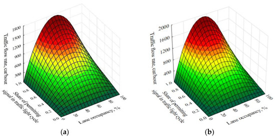
Figure 1.
The combined influence of lane occupancy and traffic light cycle on the traffic flow rate: (a) in a left-turn: (b) forward directions of the traffic flow.
From the point of view of the authors, the following results, obtained at the previous research stage, are identified as the most significant. By their physical meaning, the values of the lane occupancy indicator, which is the main and, so far, the only indicator for assessing the concentration of traffic flow in time, are always strictly in the range of 0 to 100%. When lane occupancy assumes a minimum allowable value equal to 0%, it indicates that there are no vehicles in the lane under consideration. On the contrary, a maximum allowable value of lane occupancy equal to 100% indicates that there are vehicles in the traffic lane under consideration and that the movement of the traffic flow has been completely stopped during the entire measurement period. In practice, such a cessation of traffic can occur for a number of reasons, among which the most common are the formation network congestion inside an intersection, a vehicle stopping in a traffic lane due to breakdown and, as a result, blocking the movement of the rest of the traffic flow moving along the same lane, or a traffic accident, inter alia.
Among the results obtained, the most significant from the point of view of the authors is that a new optimization criterion was established for managing traffic flows at controlled city intersections. This criterion is the optimal value of lane occupancy at which the maximum possible value of the traffic flow rate at the exit of the controlled intersection is achieved.
This is explained by the fact that as the value of lane occupancy increases, the traffic flow rate also increases. The joint increase in the values of these indicators occurs only from zero to the maximum point. Finding the values of the studied traffic flow indicators in this sector indicates a surplus in the capacity of the section of the road network under consideration. In the future, this can be used as a reserve for redistributing time between different directions of traffic flow.
However, after reaching the optimal value of lane occupancy and with its subsequent increase to 100%, the traffic flow rate only decreases from its maximum to zero. After the optimal value of lane occupancy is reached, its subsequent increase no longer causes an increase, but a decrease in the intensity of the traffic flow. This is preconditioned by the physical meaning of the model (1) and directly affected by the indicator of lane occupancy itself. In aggregates, this also indicates a decrease in the traffic capacity.
Thus, the results obtained at the previous stage of the study established that a further increase in the efficiency of the traffic organization of city road networks will be associated with the management of traffic flows by optimizing the operation of controlled intersections according to the criterion of the optimal value of lane occupancy.
2.2. Main Methodological Stages of Further Research and Their Rationale
Since the purpose of this study is to develop a practical application for the established patterns and subsequent evaluation of the effectiveness of the measures proposed, from the point of view of the authors, the main stages of the study should be as follows:
- Determining the area of practical application of the mathematical model (1), which describes the process of changing the traffic flow rate under the influence of lane occupancy at urban controlled intersections. First of all, this stage implies general analysis of existing methods for the development of traffic light control cycles. Based on the results of the analysis, an existing method is selected, which can serve as a base for further research.
- The next stage, from the point of view of the authors, should be aimed at improving the basic method, taking into account the mathematical model (1).
- This stage, according to the authors, will consist in determining the sequence of the main stages of the proposed method, taking into account lane occupancy.
- The final stage of this study will be an assessment of the effectiveness of the pro-posed method.
2.3. Determination of the of Practical Application Area of the Research Results
Traffic flow management in cities is carried out by changing the duration of traffic lights at signal-controlled intersections. Therefore, the main area for practical application of the results of the study is the adjustment of the traffic signal cycles of controlled intersections, taking into account the different incidences of lane occupancy.
Currently, there are various methods for developing and adjusting traffic signal cycles [11,41,42,43,44]. The F. Webster method can be considered the main method for designing the operation of signal-controlled intersections.
The main steps of this method are:
- Collecting the initial data on the existing traffic organization scheme and the geometric characteristics of the intersection, including traffic and pedestrian flow monitoring.
- Analyzing the data obtained, and developing and adjusting the traffic management scheme and the scheme for the traffic priority of vehicles and pedestrians.
- Determining the saturation flow (cars/hour).
- Determining the values of the phase coefficients .
- Determining the duration of the intermediate timings (s).
- Determining the duration of the traffic signal cycle (s).
- Determining the duration of the main timings (s).
- Checking the results obtained in paragraphs 5 and 7 according to compliance with the minimum required time for the movement of pedestrian flows, and adjusting the results obtained, if necessary.
The method [44] is adequate and quite applicable in the initial design of traffic lights. However, in situations where, due to an excess of lane occupancy, there is a decrease in traffic flow rate at the exit of the controlled intersection [3,4], it is not possible to adjust the traffic signal cycle according to the existing F. Webster method [44].
In this regard, in order to develop a new method, the existing procedure for determining the traffic signal cycle needs to be analyzed and improved, taking into account the results of the study.
2.3.1. Initial Data Collection
Street video surveillance cameras were used as road detectors [45], since they provide a larger viewing angle to detect vehicles in the entire functional area of the intersection and adjacent road sections under dynamic conditions (Figure 2). Street cameras are usually located on the facades of residential buildings with an elevation angle of 30–60° to the horizon and a height of 14–40 m. The video streams of these cameras support a resolution of 1920 × 1080 pixels and provide stable transmission at 25 frames per second. The determination of the occupancy and traffic intensity along the lanes from the video stream provides a solution to complex problems arising from the non-perpendicular direction of the camera view center and the large number of possible traffic scenarios. We used an optimized YOLOv4 recurrent neural network and the open-source Sort library to process the video streams, in order to detect and track multiple objects in video sequences [16]. In order to detect vehicles in control zones, we applied a method based on mapping coordinates from the camera image onto the space of the geographical coordinates using perspective transformations [46,47]. As a result of the experiment, we determined that the maximum time spent detecting a vehicle for one frame was 0.066 s.
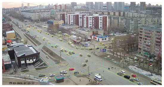
Figure 2.
An example of processing an input image and marking the boundaries of the control zones.
In order to assess the occupancy and traffic intensity along the lanes, we determined the time when the vehicle entered the control zone and calculated the accumulated distance before it left the measured zone at each i-th step of obtaining a frame from the video stream (Figure 3). The first step is to get the coordinates of the screen from the tracker. The second is the transformation of coordinates into geographical and calculation.
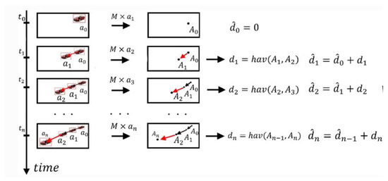
Figure 3.
Matrix of perspective transformation to determine the time spent by the vehicle within the control zone, where ai is the coordinates of a specific vehicle; di is the distance between two points; and ti is the time between frames.
The processing of each video stream frame while updating the data on the distance traveled by the vehicle allows use of the proposed method in real-time traffic control tasks (Figure 4 and Figure 5).
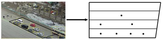
Figure 4.
Transportation of vehicle screen coordinates into geographic coordinates using perspective transformation.
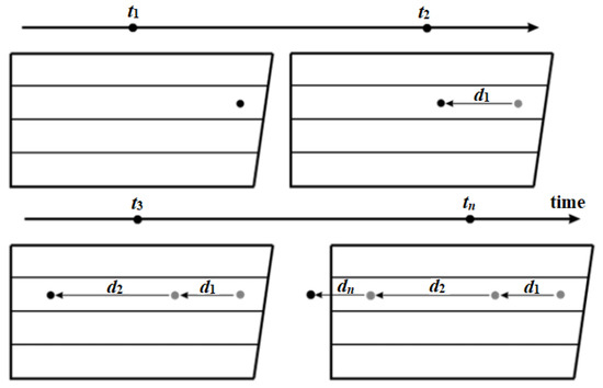
Figure 5.
Vehicle movement on a series of frames, where xi and yi are the coordinates of a specific vehicle; di is the distance between two points; and ti is the time between frames.
In order to assess the occupancy and traffic intensity along the lanes for each vehicle, we calculated the total time of its stay in the control zone (Figure 4). To this end, the location of the vehicle in the control zone was determined at each time interval. If the current (, ) and the previous coordinate (, ) are located in the zone, the time spent in the zone is taken as equal to the time between frames and considered in the total time (Figure 5). If one of the coordinates, (, ) or (, ), is beyond the control zone, the speed of the vehicle in this section is calculated using the formula:
The time spent by the vehicle in the zone is calculated using the formula:
where are the coordinates of the intersection of the travel path and the zone.
Lane occupancy is calculated using the following formula:
where θ is lane occupancy (%); n is the number of frames during which the vehicle was partially or fully in the control zone; k is the number of frames during which the vehicle was partially in the control zone; ti is the time between frames (s); is the time during which the vehicle was in the control zone between frames, (s); and is the measurement duration (s).
2.3.2. Analysis of the Data Obtained, Adjustment of the Scheme of Traffic Organization and Traffic Priority of Vehicles and Pedestrians
The traffic priority of vehicles and pedestrians, the maximum permitted speed and the direction of movement of vehicles in lanes, as well as the location of pedestrian crossings, are significant factors affecting the level of road safety. Therefore, in order to further develop the method to prevent reductions in the level of road safety, the authors introduce an additional restriction in terms of changing the traffic organization scheme and traffic priority of vehicles and pedestrians at a signalized intersection.
2.3.3. Determination of the Saturation Flow and Phase Coefficients
Saturation flow is determined by a calculation method based on the geometric characteristics of the considered intersection. The calculation method is adopted to determine the value of MS, which also allows it to reflect the effects of the geometric characteristics of the road network [19,41].
Further, the obtained calculation results will allow for determination of the coefficient y for each phase of the traffic signal cycle as the ratio of the traffic flow intensity to the value of the saturation flow.
2.3.4. Determination of the Duration of Intermediate Timings
The duration of intermediate timings in each phase of the traffic light cycle is determined according to the formula [11,19,41,44]:
where is the duration of the intermediate timing of the -th phase of the traffic signal cycle (s); ua is the average speed of vehicles on the approach to the intersection without braking (km/h); aT is the average deceleration of the vehicle when the prohibiting signal is turned on (m/s2); is the distance from the “stop line” road marking to the farthest conflict point moving in the direction in the -th phase of the traffic signal cycle (m); la is the most common value of the length of the vehicle in the flow (m); and the constants 7.2 and 3.6 are necessary for the transition to common measurement units of distance and time.
In practice, aT can be considered a constant in a range of values from 3 to 4 m/s2. The values ua, la and li are also considered constants within each phase of traffic signal control. The key operation in performing calculations is the correct determination of the distance . Unlike the durations of permitting (prohibiting) traffic signals, which can dynamically change throughout the day according to changes in transport demand, the duration primarily depends on the geometric characteristics of the road network. Therefore, can be considered constant and independent of the transport demand at the controlled intersection under consideration.
2.3.5. Determination of the Duration of the Traffic Signal Cycle
Based on the values obtained of the phase coefficients and the duration of the intermediate timings, we can calculate the optimal duration of the traffic signal cycle as follows [11,19,41,44]:
where is the duration of the traffic signal cycle (s); is the total duration of the lost time in the cycle (s); is the phase coefficient of the -th phase of the traffic signal cycle; is the number of phases in a traffic signal cycle; and the coefficients 1.5 and 5 are the reserve of the traffic light cycle time and the green signal according to [44,48,49,50,51,52].
2.3.6. Determination of the Duration of the Main Timing of the Traffic Signal Cycle
The obtained value of the cycle duration allows us to determine the duration of the main timing of each phase of the traffic signal cycle [11,19,41,44]:
where is the duration of the main timing of the -th phase of the traffic signal cycle (s).
2.3.7. Verification of Calculations, Taking into Account the Movement of Pedestrian Flows
According to (5) and (7), the calculations for traffic flows must be compared with the minimum required duration of the main and intermediate timings for pedestrian flows [11,19,41,44]:
where is the minimum required duration of the intermediate timing for the pedestrian direction in the -th phase of the traffic signal cycle (s); is the speed of the pedestrian flow (m/s); is the width of the carriageway crossed by pedestrians in the -th phase of the traffic signal cycle (m); is the minimum required duration of the signal of the main timing for the pedestrian direction in the -th phase of the traffic signal cycle (s); 4 is used to correct the speed of pedestrian traffic in order to have time to leave the carriageway during the green signal; and 5 is the additional time laid down to minimize the influence of possible additional factors on the change in the speed of pedestrian flow [11,19,41,44].
For the values obtained according to (5) and (7), the following conditions must be satisfied:
Satisfying the conditions in (10) and (11) is necessary to ensure the safe movement of pedestrians. Therefore, if the results of calculations according to (5) and (7) do not satisfy conditions (10) and (11), the duration of the main and intermediate timings for traffic flows are taken to be equal to (8) and (9), respectively.
2.3.8. Evaluation of Signal-Controlled Intersection Efficiency
A technological indicator of signal-controlled intersection efficiency is the average delay of vehicles when passing through the intersection [11,19,20,41,44]:
where is the average delay of each vehicle in the -th direction of movement (s/car); is the duration of the traffic signal cycle (s); is the ratio of the permitting traffic signal duration to the total duration of the traffic signal cycle of the -th phase of the traffic signal cycle; is the degree of saturation of the -th traffic direction; is the car traffic flow rate of the -th direction at the entrance of the controlled intersection (cars/hour); is the saturation flow in the -th phase of the -th traffic direction of vehicles (cars/hour); and 2, 1 and 0.65 are the coefficients that were obtained by F. Webster [44] based on analytical and experimental studies. The first term in (12) takes into account the regularly arriving part of the traffic flow. The second term additionally takes into account the random nature of the arrivals. The third term adjusts at least 10% of the possible error in the calculation of the delay compared to the actual experimental values.
The average delay represents the average time that each vehicle is forced to remain idle when passing through the intersection due to the operation of the traffic signal controls.
2.4. Development of a Method for Improving the Efficiency of Traffic Management at Signal-Controlled City Intersections, Taking into Account Lane Occupancy
Based on the results of the analysis of the method [44] for the development of the operating mode of the controlled intersection and taking into account the restrictions introduced to prevent a decrease in the level of road safety, the key stages of the developed method will be to adjust the following parameters of the traffic signal cycle: the phase coefficients , the total duration of the traffic signal cycle and the duration of the main timings of the cycle phases .
2.4.1. Adjustment of Phase Coefficients, Taking into Account Lane Occupancy
Taking into account (1), Formula (7) will have the form:
where is the phase coefficient of the -th phase of the traffic signal cycle, taking into account lane occupancy; is the traffic flow rate at the entrance of the controlled intersection in the -th phase along the k-th car traffic lane (cars/hour); is the traffic flow rate at the exit of the controlled intersection in the -th phase along the -th car traffic lane, influenced by the occupancy of the -th lane (cars/hour); is the saturation flow in the -th phase of the k-th traffic direction of vehicles (cars/hour); is the occupancy of the -th lane at the exit of the signal-controlled intersection (%); is the optimal lane occupancy at which the maximum value is realized in the -th phase along the -th lane, determined as a result of theoretical and experimental studies [1] (%).
It should be noted that a special case for (13) is a situation in which for the traffic lane under consideration at the signal-controlled intersection. Based on the results of theoretical studies in [1], it was found that this situation indicates a complete cessation of traffic flow along the lane under consideration. The value of the traffic flow rate at the exit of the signal-controlled intersection along this lane will be equal to zero, which was also revealed as a result of theoretical studies and was experimentally confirmed. Therefore, when such a situation occurs, the cycle should be adjusted, taking into account the exclusion of this lane from the calculations based on the complete loss of its functionality.
2.4.2. Determination of Optimal Traffic Signal Cycle Duration, Taking into Account Lane Occupancy
The values of the phase coefficients, adjusted for lane occupancy, make it possible to determine the optimal duration of the traffic signal cycle:
where is the duration of the traffic signal cycle, taking into account lane occupancy (s), and is the phase coefficient of the -th phase of the traffic signal cycle, taking into account lane occupancy.
An Additional Problem in Determining the Optimal Duration of the Traffic Signal Cycle and a Method of Solving It
The results of the analysis showed that at present, the movement of traffic flows on the road networks of cities is characterized by a significant excess of transport demand in relation to transport supply. This indicates that, according to the F. Webster method [44], the calculated value . If according to (7), the duration of the traffic signal cycle , and if the value of at any , which makes it unusable for further practical application. In order to confirm this argument, a process occurs that involves changing the value of the optimal duration of the traffic signal cycle depending on the lost time and the sum of the phase coefficients; this is shown in Figure 6.
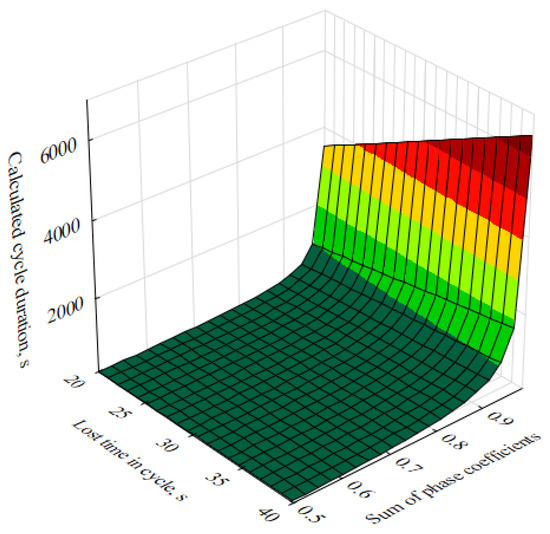
Figure 6.
Optimal traffic signal cycle duration, obtained via the F. Webster method [44], depending on the values of the sum of the phase coefficients and the lost time.
Thus, an additional task arises to determine the boundaries of the values of the minimum and maximum duration of the traffic signal cycle.
Determining the minimum allowable duration of the traffic signal cycle does not cause any difficulties. The structure of any traffic signal cycle can be represented as follows:
As indicated earlier, the value of largely depends on the geometric characteristics of the street intersection, is not subject to constant and dynamic change and it is directly related to the level of safety of road users. In this connection, the value of within the framework of a single traffic signal cycle can be considered a constant. Therefore, the structure of the minimum allowable duration of the traffic signal cycle can be represented as follows:
where is the minimum allowable duration of the traffic signal cycle (s); and is the minimum allowable duration of the main timing of the -th phase of the traffic signal cycle (s).
In turn, in each phase can be limited by the minimum required duration of the signal of the main timing in the pedestrian direction, which is determined according to (9). If in the phase under consideration, only the transport is moving, should be at least 7 s. This is due, firstly, to the purpose of ensuring the passage of at least one vehicle, which may be randomly present at the controlled intersection. Secondly, it is necessary to maintain the priority of traffic and pedestrian flows at the controlled intersection in order to ensure the safety of vehicles and pedestrians.
When determining the minimum allowable duration of the traffic signal cycle, there is no need to provide any reserve; this is because a situation where the duration of the traffic signal cycle is minimal is rather typical for inter-peak time, when transport demand tends to zero and there is no need to provide any time reserve. Therefore, it is also advisable to consider the formula for determining the minimum duration of the traffic signal cycle [11,19,41,44]:
Thus, based on (16) and (17) and taking into account (13), when adjusting the traffic signal cycle, taking into account the influence of lane occupancy, the value of the sum of phase coefficients must at least satisfy the condition:
According to (14), it is also possible to determine the boundaries of the maximum allowable values of the sum of the phase coefficients:
where is the maximum duration of the traffic signal cycle, taking into account lane occupancy (s).
Based on the results of the analyses of previously performed studies, the authors of this work have not been able to find a single approach that guarantees a positive result for determining the optimal duration of the traffic signal cycle for a fully loaded, and especially overloaded, controlled intersection.
Therefore, for the developed method, the authors of this paper propose considering as a constant that is determined by engineers and researchers independently based on their goals and priorities, as well as available reserves and resources.
In this paper, the authors decide to limit the maximum allowable duration of the traffic signal cycle to 160 s. This limit was set by Tyumen traffic engineers so that the waiting time for traffic in pedestrian flows in any redistribution of time in the traffic signal cycle does not exceed 120 s (2 min) and does not provoke pedestrians to violate traffic rules [47].
Thus, the duration of the traffic signal cycle should be within the following limits:
Therefore, if the sum of the phase coefficients obtained on the basis of (13) exceeds the maximum allowable value, it is necessary to forcibly limit it according to (20) and adjust the value of each phase coefficient. To do this, in the opinion of the authors, it is advisable to identify the specific weight of each phase coefficient of the total amount:
where is the specific weight of the phase coefficient of the -th phase of the traffic signal cycle, taking into account lane occupancy.
The value of will be applied as a correction factor and will allow us to save the specific weight of each phase coefficient, the value of which will be forcibly limited if additional adjustment is necessary:
where is the corrected value of the phase coefficient of the -th phase of the traffic signal cycle, taking into account lane occupancy.
The dependence of the maximum value of the sum of phase coefficients on lost time in a traffic signal cycle, with a different limit set on the maximum duration of the traffic signal cycle, is shown graphically in Figure 7.
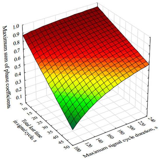
Figure 7.
The dependence of the maximum value of the sum of phase coefficients on lost time and the maximum duration of the traffic signal cycle.
2.4.3. Determination of the Duration of the Main Timings of the Traffic Signal Cycle Phases, Taking into Account Lane Occupancy
The obtained values of the duration of the traffic signal cycle and the phase coefficients will allow us to determine the duration of the main timing of each phase of the traffic signal cycle, taking into account the influence of lane occupancy:
where is the duration of the main timing of the -th phase of the traffic signal cycle, taking into account lane occupancy.
3. Results
3.1. Determination of the Main Stages of the Method for Improving the Efficiency of Traffic Management at Signal-Controlled Urban Intersections, Taking into Account Lane Occupancy
Ultimately, the developed method will include the following key stages.
- Collecting the initial data:
The initial experimental data were collected during working hours on weekdays, taking into account several requirements and restrictions. In order to achieve maximum purity of the experiment, we chose a signal-controlled intersection where the movement of trucks is prohibited and priority lanes are provided for the movement of shuttle buses. The movement on the remaining lanes is organized strictly in one of three possible directions, i.e., only straight, only to the right, or only to the left. There are no conflict points at the studied intersection during the forward movement and turning of traffic flows. The conflict or collision of vehicles and pedestrians at a workable traffic light is not possible, since a separate movement phase is provided for pedestrians. In addition, we took into account the limitations regarding the usability of the model (1) [3]: the initial data were collected in the absence of any precipitation and with clear visibility during daylight hours.
According to the technology developed for initial data collection, data were obtained on the occupancy of lanes and the traffic flow rate at the intersection under study. The total sample is presented in Figure 8.
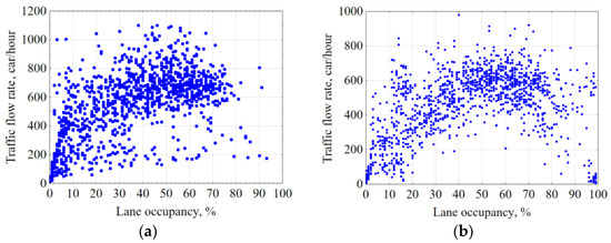
Figure 8.
Cumulative sample of initial data on traffic flow rate and occupancy of lanes in (a) left-turn and (b) forward directions of traffic flow.
- 2.
- Determining the minimum allowable duration of the main and intermediate timings and the boundaries of the duration of the traffic signal cycle.
At this stage, we calculated the values of the intermediate timings and the minimum duration of the main timings for the vehicle and pedestrian directions (, and , , respectively). A decision was made to choose the minimum allowable duration of the intermediate and main timings of each phase in order to ensure the safety of all road users. A calculation was conducted and a limit was introduced on the minimum and maximum allowable duration of the traffic signal cycle ( and , respectively).
- 3.
- Predicting the maximum possible traffic flow rate at the exit of the signal-controlled intersection.
At the same time as the previous stage, we calculated the value of the saturation flow and the share of the permitting signal for the vehicle directions of the current traffic signalization cycle. Based on the results of the calculations, as well as the data collected on occupancy , the maximum possible value of the traffic flow rate for each of the lanes at the exit of the controlled intersection was predicted. In order to do this, for each operating mode of traffic lights, the experimental data were grouped according to Sturges’ formula [53,54] for the number of intervals within a range of lane occupancy (%). Within the range, the type of distribution was determined [55], which, in most cases, corresponded to the normal distribution (Figure 9a). Using the least-square method [54,56], the regularity of the influence of lane occupancy on the traffic flow rate was established, the graphical representation of which is the regression line in Figure 9b.
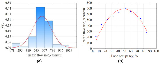
Figure 9.
The histogram and the corresponding distribution function. (a) The regularity of the influence of lane occupancy on the traffic flow rate. (b) For the traffic lights’ operating mode from 09:00 to 15:00 and from 19:00 to 23:00, λ = 0.38.
Similarly, the initial data were processed for the other modes of operation of the controlled intersection under study, operating on weekdays during the working hours of the day. Thus, for each operating mode of the controlled intersection, the maximum possible values of the traffic flow rate in the directions of movement and the optimal values of lane occupancy were predicted.
- 4.
- Determining the efficiency of traffic management at the controlled intersection with an active traffic signal cycle.
Taking into account the authors’ notion of the definition of such a phenomenon as traffic congestion, in this work, it is recommended that the traffic flow rate be taken as a key indicator to assess the effectiveness of traffic management. From the point of view of the authors, it is obvious that during the formation of a traffic jam, the value of the traffic flow rate changes at the entrance and exit of the considered system of transport nodes. Therefore, within the boundaries of the controlled intersection under consideration, the following statements are true:
where and are, respectively, the traffic flow rates at the entrance and exit of the controlled intersection (cars/hour).
It is also obvious that in the most favorable outcome, the traffic flow rate at the exit of the controlled intersection tends to the value of the flow at the entrance, but under no circumstances can it be greater. This observation allows us to represent the desired objective function of maximizing the flow rate in relative terms:
The value indicates the full satisfaction of the transport demand at the considered controlled intersection. Therefore, the current traffic signal cycle is optimal and no adjustment is required. In this case, the movement of traffic flows needs to be remonitored, in order to update the data on lane occupancy and traffic flow rate on the approach to the intersection , and then, returned to the predicting stage. When , there is a risk of traffic congestion; to prevent this, it is necessary to adjust the traffic signal cycle.
A special case for (25) would be a situation in which there is no traffic demand at all on the approach to the controlled intersection under consideration. In this case, according to the theory of limits, the efficiency value obtained by (25) is considered to be undefined on the entire number line [53]. In such a situation, the duration of the main timings of the phases of the traffic signal cycle should be adjusted to the minimum allowable duration, the values of which are determined considering the limits identified earlier in this paper.
- 5.
- Finding reserve adjustments.
An analysis was conducted of the data on lane occupancy at the exit of the controlled intersection. A decision was made on the further expediency of adjusting the traffic signal cycle. This requires that at least one of the traffic lanes in each direction be less than 100% occupied. Otherwise, it is not advisable to adjust the traffic light cycle. In order to prevent the formation of traffic congestion, the movement of vehicles at the previous controlled intersection needs to be limited by increasing the duration of the prohibitory signal or reducing the permitting signal to the minimum allowable value in directions that can facilitate the inflow of vehicles to fully occupied lanes. After that, additional monitoring of the movement of traffic flows needs to be carried out. The traffic flow rate data on the approach to the intersection and lane occupancy also need to be updated, and then, returned to the prediction stage.
- 6.
- Adjusting the traffic signal cycle.
Based on the results obtained at the previous stages, the phase coefficients were determined, as well as the duration of the traffic signal cycle and the duration of the main timings of the phases , taking into account the actual influence of the occupancy of the lanes. The adjusted cycle was put into action.
- 7.
- Analyzing the results of the adjustment.
After the cycle was introduced, the proposed adjustment was assessed. The change in the efficiency of traffic management, i.e., the difference between the value of the share of satisfied transport demand after and before the adjustment, was analyzed. The value of indicates that there has been an increase in the efficiency of traffic management and, therefore, the adjustment has been successful. If the proposed measures did not bring the expected result, like in paragraph 5 of this method, arriving vehicles at the approach to the intersection need to be limited and additional monitoring of the movement of traffic flows carried out. The traffic flow rate data on the approach to the intersection and lane occupancy need to be updated, and then, returned to the stage of predicting the rate of the outgoing traffic flow.
In contrast to the existing recommendations on the development of the operating modes of controlled intersections, when developing a traffic signal cycle according to the method proposed, not only is the presence of reserves due to incomplete loading of the road network taken into account, but it is also predicted that the maximum possible traffic flow rate at the exit of controlled intersections will decrease due to the influence of lane occupancy.
3.2. Evaluation of the Efficiency of the Developed Method
3.2.1. Evaluation of Technological Efficiency
When analyzing formula (12) to determine the average delay of the basic method of F. Webster [44], it should be noted that the product in the denominator of the degree of saturation reflects the capacity of the controlled intersection, and hence, the maximum traffic flow rate at the exit from it. Taking into account the results of the study [1], when determining the delay, we must also take into account lane occupancy, since the limitation of occurs not only due to the presence of traffic signalization means, but also due to the influence of lane occupancy . Thus, the determination of the degree of saturation and the average delay of vehicles passing through a controlled intersection, taking into account the limitation of the maximum due to the influence of lane occupancy, will have the form:
where is the average delay of each vehicle in the -th lane, taking into account lane occupancy (s/car), and is the degree of saturation of the -th lane, taking into account lane occupancy.
A special case for determining the degree of saturation would be a situation in which . In this case, the movement of vehicles along the lane is completely stopped. In other words, Qexit = 0 veh./h. Therefore, when such a situation occurs, it is proposed to exclude the lane from the calculations, and redistribute the incoming traffic evenly to the remaining lanes, along which the direction of movement of cars corresponds to the direction of movement along the fully occupied lane.
The determination of the average movement delay for each vehicle, performed according to (26), will determine the total delay for all vehicles passing through the controlled intersection:
where is the total delay in the movement of cars passing through the controlled intersection, taking into account lane occupancy (s).
The value of can be interpreted as the total idle time or the total time loss for cars, caused by the operation of traffic signalization at the intersection. Therefore, the technological effect of the application of the developed method will be as follows:
where is the technological effect of reducing the total delay in the movement of cars, obtained as a result of applying the developed method (s), and is the total delay in the movement of cars at the controlled intersection with the current traffic signal cycle before the application of the developed method (s).
Figure 10 graphically presents a comparative analysis of the current operating mode of the signal-controlled intersection and the results of adjusting the traffic light cycle according to the methodology developed, using one of the working days as an example.
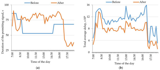
Figure 10.
Operation of the regulated intersection before and after adjustment: (a) the duration of the resolving signal of the left-turn direction; (b) the total average delay of vehicles.
3.2.2. Evaluation of Economic Efficiency
In the opinion of the authors, the economic effect of the application of the developed method will primarily be expressed in decreased fuel consumption in the idle mode of the engine, which will be realized due to a reduction in the downtime of cars when passing through a controlled intersection:
where is the total fuel consumption at idle for the time period (l), and is the nominal fuel consumption of an idle car (L/hour).
3.2.3. Evaluation of Environmental Efficiency
The authors believe that the environmental effect of the application of the developed method will be expressed as a reduction in emissions of the harmful substances , , and , which will be implemented by reducing downtime at idle speed of the car engine when driving through a signal-controlled intersection. Based on the results of studies previously conducted in this area [57,58,59,60,61,62,63,64,65,66], it seems possible to assess the expected environmental effect as follows:
where is the total reduction in emissions of the harmful substances , , and over a period of time (kg); is the specific emission of the -th harmful substance (, , or ) (kg/h); and is the technological effect of reducing the total delay in the movement of cars, obtained as a result of applying the developed method (hours).
Table 3 presents an example of evaluating the efficiency of the proposed solutions for one of the studied days of the week when the initial data were collected.
Table 3.
Comparative analysis of the efficiency of the signal-controlled intersection under the current operating parameters of traffic lights and the adjustment of the cycle according to the developed methodology using an example of the left-turn direction of traffic flow.
The data presented in Table 3 show that the application of the proposed methodology will improve the efficiency of signal-controlled intersections in all respects by an average of 35% compared to the current mode.
According to preliminary calculations, the adjustment of traffic signal cycles at the regulated intersection will reduce the total average delay in the movement of vehicles by about 127 h per working day of the week. Thus, with an average fuel cost of 95, or USD 0.64, per 1 L in Tyumen (price for the first quarter of 2022 [56]), the expected economic effect if this methodology will be more than USD 70 per 1 working day of the week. For signal-controlled intersections that are not equipped with the necessary equipment to apply the developed method, the payback period will be approximately 3.5 calendar years. The estimated reduction in emissions of harmful substances, in total, will be more than 1.6 kg for one working day of the week.
4. Discussion
The authors of this study suggest that one of the ways of resolving the problem of traffic congestion is through the management of traffic flows at signal-controlled intersections that are equipped with automated traffic control systems [16,17,18] and form part of a single urban intelligent transport system [5,6,7,8,9,10,11,12,13,14,15,16]. Decision-making regarding the particular duration of traffic signals in this concept will be based on the initial data of traffic flow rate, obtained in real time using street video surveillance cameras and neural network technologies [3,4,9,16,41].
However, the use of the traffic flow rate indicator alone is not enough to implement the control process, since both in the case of a traffic congestion and in the event of an actual decrease in transport demand in the studied lane, the detector will record a drop in the traffic flow rate value. This leads to uncertainty and does not allow the implementation of the control process. In order to resolve this uncertainty, the authors use an indicator of the concentration of traffic flow in time—lane occupancy. This indicator is essentially an indicator of the state of traffic flow, embodying the specific amount of time, from the total time resource of the lane, that the traffic flow spends on moving along the city’s road network, including acceleration, movement, deceleration and stopping [3].
The lane occupancy indicator was determined as the most useful. At the previous stage of the work, the authors conducted a study wherein the results established and experimentally confirmed a two-factor mathematical model of the effect of lane occupancy and the traffic signal cycle on the traffic flow rate [3]. The authors acknowledge that, like any other results of the study, the mathematical model obtained also has a number of limitations, and, for example, does not take into account the negative impact of environmental conditions and the quality of the road surface. However, from the point of view of the authors, the mathematical model developed is significant and allows us to continue studying both its refinement in terms of factors previously unaccounted for, and its practical application.
As a basis for developing a method for the practical application of the previously obtained mathematical models [31], the method presented in the works of F. Webster [44] was chosen. Based on the results of a detailed analysis of the method of F. Webster, a drawback was identified which does not allow for the application of this technique in modern conditions. Thus, if the transport demand exceeds the capacity of the road network, a traffic signal cycle cannot be developed using the original method. In this situation, the estimated duration of the cycle either takes on an infinitely large and unrealizable value in practice, or has no physical meaning at all, taking on a negative value. This drawback is clearly presented by the authors in Figure 6. Unfortunately, according to the authors, it is not possible to find an absolutely ideal solution in this case. As one of the solutions, the authors proposed consideration of the maximum allowable cycle duration as a constant value to be determined by an engineer or researcher, depending on the available reserves and resources, as well as their goals and objectives. This decision can be justified by the fact that in the current traffic conditions in cities, in the event of traffic congestion and the absence of any reserves for the redistribution of time in the traffic signal cycle, it will still not be possible to satisfy the entire transport demand in the road network. The authors suggest that a definitive solution to this problem is possible only when the complete redistribution of transport demand, from individual transport to alternative modes of transportation, is taken into account. However, this approach, firstly, requires long-term strategic decisions, and secondly, it still does not exclude the formation of traffic congestion due to stochastic factors, which also requires prompt adjustment of the traffic signal cycles of controlled intersections.
The authors also acknowledge that the achievement of the indicated effects of the application of the developed method can be guaranteed only if it is subject to a number of limits. These limits were justifiably introduced at the previous stage of this study during the development of the mathematical models [3]. In this regard, the positive effect of the application of the method can be realized under the condition that vehicles are moving on a dry road surface, in the absence of ice, precipitation and fog.
Vehicles moved at the intersection in strictly defined directions, where traffic flows were homogeneous and consisted only of cars. At the same time, the movement of vehicles was organized in such a way as to exclude conflict points for traffic flows moving forward and turning. Thus, the use of the proposed methodology at urban signal-controlled intersections with traffic conditions that differ from those presented in the study may require additional calibration of the mathematical models.
Therefore, improving the obtained method—taking into account the influence of various environmental conditions, the state of the road surface, the priority of public transport and other factors that can be established in the aggregate—will be an area of further research in the near future.
The prospects of the proposed methodology can be achieved through the proposed neural network technology for collecting and processing the initial data. Depending on the viewing angle, outdoor cameras track and classify vehicles within road sections of up to 500 m. Precise and informative monitoring of the dynamic parameters of traffic flows and lane distribution enables proactive adjustment of traffic lights, taking into account the individual characteristics of intersections.
5. Conclusions
The proposed method, developed on the basis of F. Webster, enables changes in traffic flow rate due to the influence of lane occupancy at urban controlled intersections to be taken into account. The developed method is based on mathematical models [3] which allow significant advancement of the existing fundamental provisions for designing operating modes for controlled intersections.
Firstly, the new method, in contrast to the existing one, takes into account the change in the maximum possible value of the traffic flow rate at the exit of the controlled intersection due to the deviation of lane occupancy from its optimal value [3,4]. In turn, this indicates either a shortage or a surplus in the traffic capacity of the road network and allows prompt real-time adjustment of the traffic light cycle at the controlled intersection in question.
Second, a detailed analysis of the basic method of F. Webster also revealed that it has another significant drawback which, in principle, does not allow its use it in modern traffic conditions in cities. With all the coherent logic of the original methodology, the calculation results obtained by it are inadequate or completely devoid of physical meaning for controlled intersections with high traffic demand. This drawback was eliminated by introducing a limit on the maximum allowable duration of the traffic light control cycle, determining the specific weight of each phase coefficient and adjusting their values, taking into account the indicated limitation.
Thirdly, in order to collect initial data on the required characteristics of traffic flows, the authors proposed an approach that consists of processing a video image received in real time from street surveillance cameras using an optimized recurrent neural network. The advantage of this approach is significant reduction in the monetary costs required for the collection of the initial data, since each street video surveillance camera is able to replace all the necessary vehicle detectors. In addition, reducing the time required to process video information makes it possible to increase the efficiency of not only monitoring the initial situation itself, but also managing traffic flows in real time.
Fourthly, it was not possible to adequately assess the efficiency of the traffic light cycle using the basic method of F. Webster, since Formula (12) for determining transport delay also did not take into account the decrease in the maximum possible traffic flow rate due to the influence of lane occupancy. In this regard, the original formula for determining the transport delay was also refined (29). This allowed for correct assessment of the efficiency of the proposed solutions. According to the preliminary results, the application of the proposed method will make it possible to realize positive technological, economic and environmental effects at urban controlled intersections.
Ultimately, a new method was developed and presented, aimed at improving the efficiency of traffic management at urban signal-controlled intersections through the real-time adjustment of traffic light cycles.
Meanwhile, we note that the accurate and situational assessment of lane occupancy is essential to ensuring effective traffic control at signal-controlled intersections. These preliminary experimental studies have shown that even when taking into account the introduced restrictions, the use of the proposed methodology can reduce the total delay of vehicles by an average of 3%. Therefore, in our future research, we will obtain more suitable parameters for adjusting traffic lights, taking into account the individual characteristics of intersections.
Author Contributions
Conceptualization, V.M.; methodology, V.M.; validation, V.M., V.S. and V.K.; initial data collection technology, V.S.; as author of the vast majority of the previous research stage, V.M. determined the areas of its practical application, analyzed the most common method of designing controlled intersections, identified its strengths and weaknesses, and developed a new method based on it; economic efficiency evaluation, V.M. and V.S.; environmental efficiency evaluation, V.M. and V.K. All authors have read and agreed to the published version of the manuscript.
Funding
This research received no external funding.
Institutional Review Board Statement
Not applicable.
Informed Consent Statement
Not applicable.
Acknowledgments
This article was prepared as part of the implementation of a state assignment in the field of science for scientific projects carried out by teams of researchers in scientific laboratories of higher educational institutions subordinate to the Russian Ministry of Education and Science, on the project: “New patterns and solutions for the functioning of urban transport systems in the paradigm “Transition from owning a personal car to mobility as a service”” (No. 0825-2020-0014, 2020–2022).
Conflicts of Interest
The authors declare no conflict of interest.
References
- Vuchic, V.R. Transportation for Livable Cities, 1st ed.; Routledge: New York, NY, USA, 2017; p. 378. [Google Scholar]
- Shepelev, V.; Aliukov, S.; Nikolskaya, K.; Shabiev, S. The capacity of the road network: Data collection and statistical analysis of traffic characteristics. Energies 2020, 13, 1765. [Google Scholar] [CrossRef]
- Morozov, V.; Iarkov, S. Formation of the Traffic Flow Rate under the Influence of Traffic Flow Concentration in Time at Controlled Intersections in Tyumen, Russian Federation. Sustainability 2021, 13, 8324. [Google Scholar] [CrossRef]
- Morozov, V.; Iarkov, S. The application of lane occupancy parameter for solving tasks of traffic management. Transp. Res. Procedia 2018, 36, 520–526. [Google Scholar] [CrossRef]
- Zhankaziev, S. Current trends of road-traffic infrastructure development. Transp. Res. Procedia 2017, 20, 731–739. [Google Scholar] [CrossRef]
- Asensio, Á.; Blanco, T.; Blasco, R.; Marco, Á.; Casas, R. Managing emergency situations in the smart city: The smart signal. Sensors 2015, 15, 14370–14396. [Google Scholar] [CrossRef]
- Cottrill, C.; Derrible, S. Leveraging big data for the development of transport sustainability indicators. J. Urban Technol. 2015, 22, 45–64. [Google Scholar] [CrossRef]
- Errampalli, M.; Chalumuri, R.S.; Nath, R. Development and evaluation of an integrated transportation system: A case study of Delhi. Proc. Inst. Civ. Eng. Transp. 2018, 171, 75–84. [Google Scholar] [CrossRef]
- Karmanov, D.S.; Zakharov, D.A.; Fadyushin, A.A. Evaluation of changes in traffic parameters for various types of traffic signal regulation. Transp. Res. Procedia 2018, 36, 274–280. [Google Scholar] [CrossRef]
- Krivolapova, O. Algorithm for Risk Assessment in the Introduction of Intelligent Transport Systems Facilities. Transp. Res. Procedia 2017, 20, 373–377. [Google Scholar] [CrossRef]
- Moroz, B.I.; Udovyk, I.M.; Shvachych, G.G.; Pasichnik, A.M.; Miroshnichenko, S.V. Intelligent system of traffic light control with dynamic change phases of traffic flows on controlled intersections. Sci. Rev. 2019, 1, 11–17. [Google Scholar] [CrossRef]
- Nguyen, D.D.; Rohács, J.; Rohács, D.; Boros, A. Intelligent Total Transportation Management System for Future Smart Cities. Appl. Sci. 2020, 10, 8933. [Google Scholar] [CrossRef]
- Petrov, A.I.; Kolesov, V.I.; Petrova, D.A. Theory and Practice of Quantitative Assessment of System Harmonicity: Case of Road Safety in Russia before and during the COVID-19 Epidemic. Mathematics 2021, 9, 2812. [Google Scholar] [CrossRef]
- Rodríguez, D.A.; Levine, J.; Agrawal, A.W.; Song, J. Can information promote transportation-friendly location decisions? A simulation experiment. J. Transp. Geogr. 2010, 19, 304–312. [Google Scholar] [CrossRef]
- Shepelev, V.D.; Glushkov, A.I.; Almetova, Z.V.; Mavrin, V.G. A study of the travel time of intersections by vehicles using computer vision. In Proceedings of the 6th International Conference on Vehicle Technology and Intelligent Transport Systems, Online, 2–4 May 2020; pp. 653–658. [Google Scholar]
- Shepelev, V.; Zhankaziev, S.; Aliukov, S.; Varkentin, V.; Marusin, A.; Marusin, A.; Gritsenko, A. Forecasting the Passage Time of the Queue of Highly Automated Vehicles Based on Neural Networks in the Services of Cooperative Intelligent Transport Systems. Mathematics 2022, 10, 282. [Google Scholar] [CrossRef]
- Khazukov, K.; Shepelev, V.; Karpeta, T.; Shabiev, S.; Slobodin, I.; Charbadze, I.; Alferova, I. Real-time monitoring of traffic parameters. J. Big Data 2020, 7, 84. [Google Scholar] [CrossRef]
- Winter, H.; Serra, J.; Nesmachnow, S.; Tchernykh, A.; Shepelev, V. Computational intelligence for analysis of traffic data. In Proceedings of the Communications in Computer and Information Science, Online, 9–11 November 2020; Volume 1359, pp. 167–182. [Google Scholar] [CrossRef]
- National Academies of Sciences, Engineering, and Medicine. Highway Capacity Manual: A Guide for Multimodal Mobility Analysis, 7th ed.; The National Academies Press: Washington, DC, USA, 2022. [Google Scholar]
- Gordon, R.L.; Tighe, W. Traffic Control Systems Handbook; U.S. Department of Transportation, Federal Highway Administration: Washington, DC, USA, 2005. [Google Scholar]
- Gerlough, D.L.; Huber, J.H. Traffic Flow Theory: A Monograph; Transportation Research Board National Research Council: Washington, DC, USA, 1975. [Google Scholar]
- Larin, O.N.; Dosenko, V.A. Use of a Phase Transition Concept for Traffic Flow Condition Estimation. Transp. Telecommun. 2014, 15, 315–321. [Google Scholar] [CrossRef][Green Version]
- Athol, P. Interdependence of Certain Operational Characteristics Within a Moving Traffic Stream. Highw. Res. Rec. 1965, 72, 58–87. [Google Scholar]
- Banks, J.H. Freeway Speed-Flow-Concentration Relationships: More Evidence and Interpretations. Transp. Res. 1989, 1225, 53–60. [Google Scholar]
- Hall, F.L.; Gunter, M.A. Further Analysis of the Flow-Concentration Relationship. Transp. Res. 1986, 1901, 1–9. [Google Scholar]
- Hall, F.L.; Hurdle, V.F.; Banks, J.H. Synthesis of recent work on the nature of speed-flow and flow-occupancy (or density) relationships on freeways. Transp. Res. 1992, 1365, 12–18. [Google Scholar]
- Hurdle, V.F.; Datta, P.K. Speeds and Flows on an Urban Freeway: Some Measurements and a Hypothesis. Transp. Res. 1983, 905, 127–137. [Google Scholar]
- Hurdle, V.F.; Merlo, M.I.; Robertson, D. Study of speed-flow relationships on individual freeway lanes. Transp. Res. 1997, 1591, 7–13. [Google Scholar] [CrossRef]
- Pushkar, A.; Hall, F.L.; Acha-Daza, J.A. Estimation of Speeds from Single-Loop Freeway Flow and Occupancy Data Using the Cusp Catastrophe Theory Model. Transp. Res. 1994, 1457, 149–157. [Google Scholar]
- Araghi, S.; Khosravi, A.; Johnstone, M.; Creighton, D. Intelligent Traffic Light Control of Isolated Intersections Using Machine Learning Methods. In Proceedings of the 2013 IEEE International Conference on Systems, Man, and Cybernetics, Manchester, UK, 13–16 October 2013; pp. 3621–3626. [Google Scholar] [CrossRef]
- Tresler, F. A proposed model of extended coordination for the traffic light control at intersections. Commun. Comput. Inf. Sci. 2012, 329, 240–248. [Google Scholar] [CrossRef]
- Gunes, F.; Bayrakli, S.; Zaim, A.H. Smart Cities and Data Analytics for Intelligent Transportation Systems: An Analytical Model for Scheduling Phases and Traffic Lights at Signalized Intersections. Appl. Sci. 2021, 11, 6816. [Google Scholar] [CrossRef]
- Harahap, E.; Darmawan, D.; Fajar, Y.; Rachmiatie, A. Modeling and simulation of queue waiting time at traffic light intersection. J. Phys. Conf. Ser. 2019, 1188, 012001. [Google Scholar] [CrossRef]
- Leverents, E.; Andronov, R.; Anufrieva, T. Simulation of queue length and vehicle delays on signal-controlled intersection. MATEC Web Conf. 2018, 170, 05010. [Google Scholar] [CrossRef][Green Version]
- Li, X.; Khattak, A.J.; Kohls, A.G. Signal phase timing impact on traffic delay and queue length-a intersection case study. In Proceedings of the Winter Simulation Conference (WSC), Washington, DC, USA, 11–14 December 2016; pp. 3722–3723. [Google Scholar] [CrossRef]
- Adak, M.F.; Balta, M. Fuzzy Logic-based Adaptive Traffic Light Control of an Intersection: A Case Study. In Proceedings of the 5th International Symposium on Multidisciplinary Studies and Innovative Technologies (ISMSIT), Ankara, Turkey, 21–23 October 2021; pp. 394–398. [Google Scholar] [CrossRef]
- Talab, H.S.; Mohammadkhani, H. Design Optimization Traffic Light Timing Using the Fuzzy Logic at a Diphasic’s Isolated Intersection. J. Intell. Fuzzy Syst. 2014, 27, 1609–1620. [Google Scholar] [CrossRef]
- Yusuf, A.M.H.; Yusuf, R. Adaptive Traffic Light Controller Simulation for Traffic Management. In Proceedings of the 6th International Conference on Interactive Digital Media (ICIDM), Bandung, Indonesia, 14–15 December 2020; pp. 1–5. [Google Scholar] [CrossRef]
- Yang, Z.; Peng, J.; Wu, L.; Ma, C.; Zou, C.; Wei, N.; Zhang, Y.; Liu, Y.; Andre, M.; Li, D.; et al. Speed-guided intelligent transportation system helps achieve low-carbon and green traffic: Evidence from real-world measurements. J. Clean. Prod. 2020, 268, 122230. [Google Scholar] [CrossRef]
- Alrawi, F. The importance of intelligent transport systems in the preservation of the environment and reduction of harmful gases. Transp. Res. Procedia 2017, 24, 197–203. [Google Scholar] [CrossRef]
- Branston, D. Some factors affecting the capacity of signalized intersection. Traffic Eng. Control 1979, 20, 390–396. [Google Scholar]
- Gorodokin, V.; Almetova, Z.; Shepelev, V. Procedure for calculating on-time duration of the main cycle of a set of coordinated traffic lights. Pap. Present. Transp. Res. Procedia 2017, 20, 231–235. [Google Scholar] [CrossRef]
- Glushkov, A.; Shepelev, V. Development of reliable models of signal-controlled intersections. Transp. Telecommun. 2021, 22, 417–424. [Google Scholar] [CrossRef]
- Webster, F.V.; Cobbe, B.M. Traffic Signals; Road Research Technical Paper N56; HMSQ: London, UK, 1966. [Google Scholar]
- Video observation: Online broadcast. Available online: https://stream.is74.ru (accessed on 8 February 2022).
- Fedorov, A.; Nikolskaia, K.; Ivanov, S.; Shepelev, V.; Minbaleev, A. Traffic Flow Estimation with Data from a Video Surveillance Camera. J. Big Data 2019, 6, 73. [Google Scholar] [CrossRef]
- Tyumen City Transport. Available online: https://tgt72.ru/ (accessed on 8 February 2021). (In Russian).
- Keilson, J. Introduction to the Theory of Queues. Technometrics 1963, 5, 286. [Google Scholar] [CrossRef]
- Krishnamoorthy, A.; Joshua, A.N.; Vishnevsky, V. Analysis of a k-Stage Bulk Service Queuing System with Accessible Batches for Service. Mathematics 2021, 9, 559. [Google Scholar] [CrossRef]
- Ma, F.-Q.; Fan, R.-N. Queuing Theory of Improved Practical Byzantine Fault Tolerant Consensus. Mathematics 2022, 10, 182. [Google Scholar] [CrossRef]
- Minkevičius, S.; Katin, I.; Katina, J.; Vinogradova-Zinkevič, I. On Little’s Formula in Multiphase Queues. Mathematics 2021, 9, 2282. [Google Scholar] [CrossRef]
- Tsitsiashvili, G. Construction and Analysis of Queuing and Reliability Models Using Random Graphs. Mathematics 2021, 9, 2511. [Google Scholar] [CrossRef]
- Hubbard, J.H.; Hubbard, B.B. Vector Calculus, Linear Algebra, and Differential Forms: A Unified Approach, 6th ed.; Matrix Editions: Ithaca, NY, USA, 2015; p. 818. [Google Scholar]
- Sturges, H. The choice of a class-interval. J. Am. Stat. Assoc. 1926, 21, 65–66. [Google Scholar] [CrossRef]
- Bhattacharya, G.K.; Johnson, R.A. Statistical Concepts and Methods; John Wiley & Sons: New York, NY, USA, 1977; p. 639. [Google Scholar]
- Federal State Statistics Service. Available online: https://eng.rosstat.gov.ru (accessed on 17 December 2021).
- Boulter, P.G.; Latham, S. Emissions Factors 2009: Report 5—A Review of the Effects of Fuel Properties on Road Vehicle Emissions; RL Report PPR358; TRL Limited: Wokingham, UK, 2009. [Google Scholar]
- Chainikov, D.; Chikishev, E.; Anisimov, I.; Gavaev, A. Influence of Ambient Temperature on the CO2 Emitted with Exhaust Gases of Gasoline Vehicles. In Proceedings of the VII International Scientific Practical Conference “Innovative Technologies in Engineering”, Yurga, Russia, 19–21 May 2016; Volume 142, p. 12109. [Google Scholar] [CrossRef]
- Magaril, E. Increasing the efficiency and environmental safety of vehicle operation through improvement of fuel quality. Int. J. Sustain. Dev. Plan. 2015, 10, 880–893. [Google Scholar] [CrossRef]
- Magaril, E.; Magaril, R.; Abrzhina, L. Environmental Assessment of the Measures Increasing the Sustainability of Motor Transport. IOP Conf. Ser. Earth Environ. Sci. 2017, 72, 012003. [Google Scholar] [CrossRef]
- Magaril, E.; Abrzhina, L.; Belyaeva, M. Environmental damage from the combustion of fuels: Challenges and methods of economic assessment. WIT Trans. Ecol. Environ. 2014, 190, 1105–1115. [Google Scholar] [CrossRef]
- Parsaev, E.V.; Malyugin, P.N.; Teterina, I.A. Methodology for the calculation of emissions for non-stationary transport flow. Russ. Automob. Highw. Ind. J. 2018, 15, 686–697. (In Russian) [Google Scholar] [CrossRef]
- Schiavon, M.; Redivo, M.; Antonacci, G.; Rada, E.C.; Ragazzi, M.; Zardi, D.; Giovannini, L. Assessing the air quality impact of nitrogen oxide and benzene from road traffic and domestic heating and the associated cancer risk in an urban area of Verona (Italy). Atmos. Environ. 2015, 120, 234–243. [Google Scholar] [CrossRef]
- Stroe, C.-C.; Panaitescu, V.N.; Ragazzi, M.; Rada, E.C.; Ionescu, G. Some considerations on the environmental impact of highway traffic. Rev. Chim. 2014, 65, 152–155. [Google Scholar]
- Zakharov, D.; Magaril, E.; Rada, E.C. Sustainability of the Urban Transport System under Changes in Weather and Road Conditions Affecting Vehicle Operation. Sustainability 2018, 10, 2052. [Google Scholar] [CrossRef]
- Ertman, S.; Ertman, J.; Zakharov, D. Adaptation of urban roads to changing of transport demand. E3S Web Conf. 2016, 6, 01013. [Google Scholar] [CrossRef]
Publisher’s Note: MDPI stays neutral with regard to jurisdictional claims in published maps and institutional affiliations. |
© 2022 by the authors. Licensee MDPI, Basel, Switzerland. This article is an open access article distributed under the terms and conditions of the Creative Commons Attribution (CC BY) license (https://creativecommons.org/licenses/by/4.0/).