Concrelife: A Software to Solve the Chloride Penetration in Saturated and Unsaturated Reinforced Concrete

Abstract

This paper presents new software (Concrelife) capable of reliably simulating chloride ions penetration in reinforced concrete from different environments in the most common 1-D rectangular geometry scenarios. Its numerical solution is obtained from the simulation of models whose structure is based on Network Simulation Method. These models are generated by the program itself and run in the powerful free code NgSpice. The mathematical model of the problem includes the formation of bound chloride, precipitated chloride, reduction of porosity, saturated and unsaturated conditions, etc. All this allows tackling all kinds of scenarios, such as successive changes in concentration and temperature at the boundary, wet-drying cycles, washing of structures, etc. Concrelife has been developed with a pleasant window environment, intuitive and easy for a user not expert in numerical techniques, both for the introduction of data and for the graphic representation of the results, which include the spatial and temporal concentration of all species of chloride, porosity, water content in pores etc. To test and verify the results of the software, applications are presented to real scenarios.

1. Introduction

Most of the civil engineering constructions are made with steel reinforced concrete. Pillars and boards of bridges, ports, oil extraction offshore facilities, etc., they are all types of structures that are frequently subjected to external liquid or gaseous environments which contain corrosive contaminants. These pollutants penetrate the concrete through different physical mechanisms (diffusion, advection, migration, capillarity ...) and, once they reach the reinforcement and overcome a certain concentration threshold, due to the alkalinity of the hydration concrete products, they break the current state of passivation of the steel and start up the armor corrosion [1,2,3,4,5,6]. This is what is generally called the first stage of the corrosion process [3,4,6]. The second stage begins at this point, with the formation of tiny bites in the steel, and continues with the appearance of chemical corrosion products that, in their expansion, cause large stresses in the concrete bulk that end in increase cracks and fractures that finally lead to the mechanical collapse of the structure [2,3,4].

As in other fields of engineering, the use of specific programs has already become a necessity because, above all, it avoids the enormous economic and time-saving cost that would require solving these problems without analytical solution through experimental techniques. This is particularly true in the problems of penetration of chlorides in concrete in which experimental tests can last for years in many cases. We focus this work on the presentation of Concrelife [7], a new numerical software for solving the problem of chloride diffusion in reinforced concretes. The program, whose models are based on the Network Simulation Method [8,9,10], is able to approach the most common 1-D rectangular domains, under boundary conditions that reproduce the exposure of the concrete sample either to liquid environments (saturated concrete) or in gaseous environments with relative humidity below 100% (unsaturated concrete), always providing reliable solutions.

Concrelife [7] is the last of a set of numerical simulation programs of similar structure and organization developed by the UPCT with teaching and research objectives. For example, FATSIM-A [11], for solving flow and mass transport in porous media, SICOMED_18 [12], for simulating soil consolidation with penetrating drains, CODENS_13 [13], for the solution of nonlinear systems of coupled ordinary differential equations or OXIPSIS_12 [14], for simulating different corrosion problems. Thanks to the use of these software, numerous research papers have been published [15,16,17,18,19,20].

The mathematical model that rules the problem in water-saturated concretes is basically form by a main diffusion equation (which contains a term that includes the effects of the change in porosity) with the free chloride concentration in the liquid solution that occupies the porous as variable and a diffusion coefficient dependent on temperature. Chloride penetration is so coupled to the problem of heat transfer in the concrete itself, also ruled by an independent diffusion equation. In addition, the formation of bounded and precipitated chloride is assumed, these are physical or chemical mechanisms ruled by complementary equations that related the bounded and free chloride (the so-called isotherms) and the concentration condition under which precipitation emerges. The formation of salts by bound chloride or precipitate crystals results in a reduction of the pore size which, in turn, influences the chloride penetration process. In the case of water-unsaturated problem, the mathematical model contains new equations that relate, on the one hand, the porosity with the pore water content and, on the other, the capillary pressure with the relative humidity of surrounding air environment. In addition, most of the parameters involved, such as density, viscosity and diffusion coefficients, are dependent on temperature and concentration through empirical expressions currently used in the scientific literature. All previous makes the mathematical model (water-saturated or not) coupled and strongly nonlinear, impossible to address by techniques other than numerical ones. Thus, numerous works propose specific numerical methods, verified to a greater or lesser degree [1,21,22,23,24,25,26,27,28,29], which are not available to the user without expertise in the field of computing. Some software use models based on the regulations (EN 12390-11:2019) [30] or similar that are based on the implementation of Fick’s second law by means of the error function, where a semi-infinite medium is assumed that is only valid for small times, so they could give results that are far from reality in the service life times. Others have designed commercial software, perhaps of less precision, that give an approximate idea of the service life times of these armor structures. This work focuses towards this last aim, where in the Concrelife software the complex coupled and strongly non-linear mathematical model has been implemented without assumptions.

Concrelife has been developed in a pleasant window environment which allows easy communication with the user both for data entry (parameters involved, boundary conditions and simulation time window) and for the representation of results in tabulated or graphical form. The user chooses the mesh size by establishing a compromise between the required accuracy and the computing time. Mesh sizes above 50 ensure generally acceptable errors in the engineering field. The Concrelife results have been verified both experimentally and by comparison with those obtained by other numerical methods, providing in all cases negligible deviations.

In what follows, the mathematical models of the saturated and unsaturated problems are firstly presented, followed by an explanation of the detailed use of Concrelife software through its user interaction windows and by the solution of two illustrative applications to real scenarios. Finally, the characteristics of the program and its potential to address the wide variety of problems related to the penetration of chlorides in reinforced concrete are synthesized.

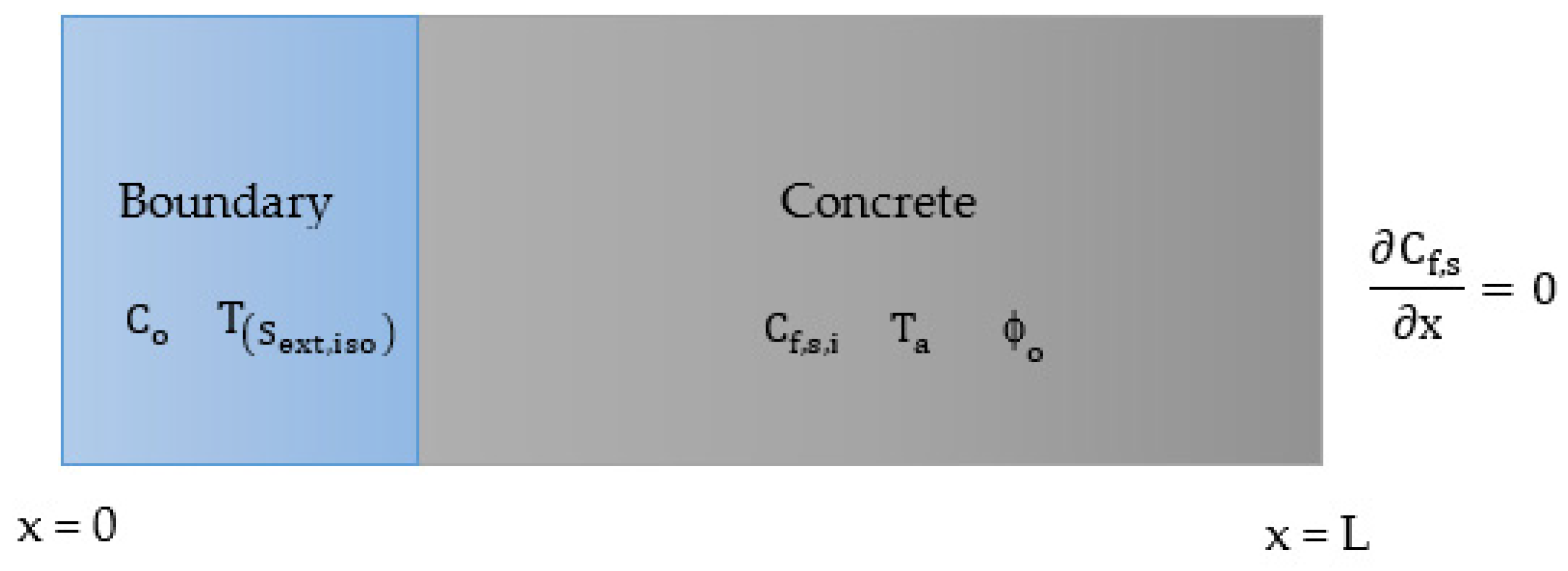
2. The Governing Equations

2.1. Water-Saturated Concrete

The mathematical model for heat and chloride transport in water-saturated concrete [1,21,24,27,31,32,33] is formed by the set of Equations (1) to (15), shown in

Table 1. Mathematical model of transport in saturated concrete.

Heat Transport
Governing equation:
$\frac{\partial \mathrm{T}}{\partial \mathrm{t}}-{\mathsf{\alpha }}_{\mathrm{T}}{\nabla }^2\left(\mathrm{T}\right)=0$	(1)
Boundary conditions:	(2)
${\mathrm{T}}_{\left({\mathrm{S}}_{\mathrm{ext},\mathrm{iso}}\right)}=\mathrm{T}\left(\mathrm{t}\right)$
${\left(\frac{\partial \mathrm{T}}{\partial n}\right)}_{\left({\mathrm{S}}_{\mathrm{ext},\mathrm{adi}}\right)}=0$,   at adiabatic contour	(3)
Initial condition:
${\mathrm{T}}_{\left(\mathrm{t}=0\right)}={\mathrm{T}}_{\mathrm{a}}$    at the domain	(4)
Chloride transport
Governing equation:
$\frac{\partial {\mathrm{C}}_{\mathrm{t},\mathrm{c}}}{\partial \mathrm{t}}+\nabla ·\left({\mathrm{D}}_{\mathrm{c}}{\mathrm{C}}_{\mathrm{f},\mathrm{s}}\nabla {\mathsf{\varphi }}_{\mathrm{l}}\right)=\nabla ·\left({\mathrm{D}}_{\mathrm{c}}\nabla {\mathrm{C}}_{\mathrm{f},\mathrm{c}}\right)$	(5)
${\mathrm{C}}_{\mathrm{f},\mathrm{c}}={\mathrm{C}}_{\mathrm{f},\mathrm{s}}{\mathsf{\varphi }}_{\mathrm{l}}$	(6)
${\mathrm{C}}_{\mathrm{t},\mathrm{c}}={\mathrm{C}}_{\mathrm{f},\mathrm{c}}+{\mathrm{C}}_{\mathrm{b}}+{\mathrm{C}}_{\mathrm{p}}$	(7)
${\mathsf{\varphi }}_{\mathrm{l}}={\mathsf{\varphi }}_{\mathrm{o}}-\frac{1}{{\mathsf{\rho }}_{\mathrm{F}}}{\mathrm{C}}_{\mathrm{b}}-\frac{1}{{\mathsf{\rho }}_{\mathrm{ps}}}{\mathrm{C}}_{\mathrm{p}}$	(8)
$\frac{\partial {\mathrm{C}}_{\mathrm{p}}}{\partial \mathrm{t}}=-{\mathrm{C}}_{\mathrm{f},\mathrm{s},\mathrm{sat}} \frac{\partial {\mathsf{\varphi }}_{\mathrm{l}}}{\partial \mathrm{t}} {\left(\frac{\partial {\mathrm{C}}_{\mathrm{b}}}{\partial {\mathrm{C}}_{\mathrm{f},\mathrm{c}}}\right)|}_{{\mathrm{C}}_{\mathrm{f},\mathrm{c}}={\mathrm{C}}_{\mathrm{f},\mathrm{s},\mathrm{sat}}·{\mathsf{\varphi }}_{\mathrm{l}}}$	(9)
${\mathrm{C}}_{\mathrm{f},\mathrm{s},\mathrm{sat}}=\frac{{\mathrm{C}}_{\mathrm{NaCl}}^{\mathrm{S}}{\mathrm{M}}_{\mathrm{Cl}}\left(1000+\Delta {\mathsf{\rho }}_{\mathrm{l}}^{\mathrm{T}}\right)}{1+{\mathrm{C}}_{\mathrm{NaCl}}^{\mathrm{S}}{\mathrm{M}}_{\mathrm{NaCl}}\left(1-{\mathsf{\rho }}_{\mathrm{l}}^0\mathsf{\epsilon }\right)}$	(10)
${\mathrm{C}}_{\mathrm{NaCl}}^{\mathrm{S}}=\left(6.044+2.8\times {10}^{-3}\mathrm{T}+3.6\times {10}^{-5}{\mathrm{T}}^2\right){10}^{-3}$	(11)
$\Delta {\mathsf{\rho }}_{\mathrm{l}}^{\mathrm{T}}=-1000\frac{\left(\mathrm{T}+288.9414\right){\left(\mathrm{T}-3.9863\right)}^2}{508929.2\left(\mathrm{T}+68.12963\right)}$	(12)
${\mathrm{D}}_{\mathrm{c}}={\mathrm{D}}_{\exp } {\exp }^{\left(-\frac{{\mathrm{E}}_{\mathrm{a}}}{\mathrm{R}}\left[\frac{1}{\mathrm{T}}-\frac{1}{{\mathrm{T}}_{\mathrm{o}}}\right]\right)}$	(13)
${\mathrm{C}}_{\mathrm{b}}~{\mathrm{C}}_{\mathrm{f},\mathrm{c}}$ Isotherms:
${\mathrm{C}}_{\mathrm{b}}={\mathrm{C}}_{\mathrm{b},\mathrm{o}}{\mathrm{K}\mathrm{C}}_{\mathrm{f},\mathrm{c}}$     (linear)	(14a)
${\mathrm{C}}_{\mathrm{b}}=\frac{{\mathrm{C}}_{\mathrm{b},\mathrm{o}}{\mathrm{K}\mathrm{C}}_{\mathrm{f},\mathrm{c}}}{1+{\mathrm{K}\mathrm{C}}_{\mathrm{f},\mathrm{c}}}$     (Langmuir)	(14b)
${\mathrm{C}}_{\mathrm{b}}={{\mathsf{\beta }\mathrm{C}}_{\mathrm{f},\mathrm{c}}}^{\mathsf{\alpha }}$     (Freundlich)	(14c)
${\mathrm{C}}_{\mathrm{b}}={\mathrm{C}}_{\mathrm{b},\mathrm{o}}\frac{{\mathrm{KC}}_{\mathrm{f},\mathrm{c}}^{\mathsf{\alpha }}}{1+{\mathrm{KC}}_{\mathrm{f},\mathrm{c}}^{\mathsf{\alpha }}}$   (Langmuir-Freundlich)	(14d)
Boundary conditions:
${\mathrm{C}}_{\mathrm{f},\mathrm{s}\left(\mathrm{t},{\mathrm{S}}_{\mathrm{ext},\mathrm{iso}}\right)}={\mathrm{C}}_{\mathrm{o}}$	(15)
${\left(\frac{\partial {\mathrm{C}}_{\mathrm{f},\mathrm{s}}}{\partial n}\right)|}_{{\mathrm{S}}_{\mathrm{ext},\mathrm{adi}}}=0$	(16)
Initial conditions:
${\mathrm{C}}_{\mathrm{f},\mathrm{s}\left(\mathrm{t}=0\right)}={\mathrm{C}}_{\mathrm{f},\mathrm{s},\mathrm{i}}=\frac{{\mathrm{C}}_{\mathrm{f},\mathrm{c},\mathrm{i}}}{{\mathsf{\varphi }}_{\mathrm{o}}}$	(17)
${\mathsf{\varphi }}_{\mathrm{l}\left(\mathrm{t}=0\right)}={\mathsf{\varphi }}_{\mathrm{o}}$	(18)

and Figure 1.

The heat transport equation involves Fourier law and conservation of heat flow. In the governing Equation (1) T (K) and t (s) are temperature and time, while ${\mathsf{\alpha }}_{\mathrm{T}}$ (m²s⁻¹) is the average thermal diffusivity of the porous media, the ratio between the average thermal conductivity k_m (Wm⁻¹K⁻¹) and the average specific heat (ρc_e)_m (Jm⁻³K⁻¹). In the boundary conditions Equations (2) and (3), ${\mathrm{T}}_{\left({\mathrm{S}}_{\mathrm{ext},\mathrm{iso}}\right)}$ is the time dependent temperature (a t-T table) applied to the concrete exterior surface (generally a seasonal dependence) and ${\left(\frac{\partial \mathrm{T}}{\partial n}\right)}_{\left({\mathrm{S}}_{\mathrm{ext},\mathrm{adi}}\right)}$ the temperature gradient on the adiabatic surface. T_a represents the initial temperature of the concrete, Equation (4). This heat problem is decoupled from chloride transport so that it is solved separately.

The chloride transport is ruled by a nonlinear diffusion Equation (5) in which two variables are involved, the chloride concentration and the pore solution content. In the chloride transport, ${\mathrm{C}}_{\mathrm{f},\mathrm{s}}$, ${\mathrm{C}}_{\mathrm{f},\mathrm{c}}$ and ${\mathrm{C}}_{\mathrm{t},\mathrm{c}}$ are variables that represent the free chloride concentration at the solution (kg/m³ solution), the free chloride concentration at the concrete (kg/m³ concrete) and the total chloride concentration at the concrete (kg/m³ concrete) while ${\mathrm{C}}_{\mathrm{b}}$ and ${\mathrm{C}}_{\mathrm{p}}$ are the bound and precipitated chloride concentration at the concrete (kg/m³ concrete). These chlorides are related by the definition (6) and the total chloride (mass) conservation (7). ${\mathsf{\varphi }}_{\mathrm{l}}$, the pore solution content (m³ of solution/m³ of concrete) is related by bound and precipitate chlorides by Equation (8) where ${\mathsf{\varphi }}_{\mathrm{o}}$ is initial porosity (m³ of pores/m³ of concrete), and ${\mathsf{\rho }}_{\mathrm{F}}$ and ${\mathsf{\rho }}_{\mathrm{p}.\mathrm{s}}$ the densities of Friedel’s salt (1892 kg/m³ of concrete) and precipitate (2165 kg/m³ of concrete).${\mathrm{C}}_{\mathrm{f},\mathrm{s},\mathrm{sat}}$ is the saturate concentration of the chloride solution to start the precipitation whose rate is given by Equation (9). This parameter (${\mathrm{C}}_{\mathrm{f},\mathrm{s},\mathrm{sat}}$) depends on temperature according to the expression [34], Equation (10), with ${\mathrm{C}}_{\mathrm{NaCl}}^{\mathrm{S}}$ (mol/g of water) the chloride content in a saturated solution, also temperature dependent in the form of Equation (11) [34,35,36], with T in °C. In Equation (10), ${\mathrm{M}}_{\mathrm{NaCl}}$ and ${\mathrm{M}}_{\mathrm{Cl}}$ are the molecular weight of NaCl and Cl, respectively, ${\mathsf{\rho }}_{\mathrm{l}}^0$ the density of pure water at 20 °C (${\mathsf{\rho }}_{\mathrm{l}}^0$ = 998.2 kg/m³), ε a correlation dimensional coefficient (6.46 × 10⁻⁴ m³/kg, [36]) and $\Delta {\mathsf{\rho }}_{\mathrm{l}}^{\mathrm{T}}$ the change in water density with temperature (°C) given by Equation (12) [35].

The dependence of ${\mathrm{D}}_{\mathrm{c}}$ on temperature is given by Equation (13), the only coupling with heat transport, with ${\mathrm{E}}_{\mathrm{a}}$ the activation energy of the NaCl (20 kJ according [37]. As for the dependence between ${\mathrm{C}}_{\mathrm{b}}$ and ${\mathrm{C}}_{\mathrm{f},\mathrm{c}}$, the well-known expressions of linear, Langmuir and Freundlich isotherms, Equations (14a) to (14d), are assumed. Each of them with their specific coefficients: K (m³ of concrete per kg de chloride) an equilibrium constant for Langmuir models, ${\mathrm{C}}_{\mathrm{b},\mathrm{o}}$ (kg/m³ concrete) the maximum bounded chloride ion concentration at the concrete, and α (dimensionless) and β (m³ concrete/kg)^α−1 constants at the Freundlich expressions. Finally, Equations (15) and (16) show the boundary conditions, with ${\mathrm{C}}_{\mathrm{o}}$ the free chloride concentration at the surrounding liquid, while Equations (17) and (18) are the initial condition for chloride and pore solution content, with ${\mathrm{C}}_{\mathrm{f},\mathrm{s},\mathrm{i}}$ the initial free chloride concentration in the solution (kg/m³ solution) and ${\mathrm{C}}_{\mathrm{f},\mathrm{c},\mathrm{i}}$ the initial free chloride concentration at the concrete (kg/m³ concrete). Finally, ${\mathsf{\varphi }}_{\mathrm{o}}$ is the initial porosity of the concrete.

2.2. Water-Unsaturated Concrete

Table 2. Mathematical model of transport in water-unsaturated concrete.

Heat transport:
Equations (1) to (4), Table 1
Chloride transport:
Governing equation:
$\frac{\partial {\mathrm{C}}_{\mathrm{t},\mathrm{c}}}{\partial \mathrm{t}}+\nabla ·\left({\mathrm{D}}_{\mathrm{c}}{\mathrm{C}}_{\mathrm{f},\mathrm{s}}\nabla {\mathsf{\varphi }}_{\mathrm{l}}\right)+\nabla ·\left[\left(\frac{{\mathrm{kC}}_{\mathrm{f},\mathrm{s}}}{{\mathsf{\nu }}_{\mathrm{l}}{\mathsf{\varphi }}_{\mathrm{l}}}\right)\left(\frac{\partial {\mathrm{p}}_{\mathrm{c}}}{\partial {\mathsf{\varphi }}_{\mathrm{l}}}\nabla {\mathsf{\varphi }}_{\mathrm{l}}+\frac{\partial {\mathrm{p}}_{\mathrm{c}}}{\partial \mathsf{\varphi }}\nabla \mathsf{\varphi }+\frac{\partial {\mathrm{p}}_{\mathrm{c}}}{\partial \mathrm{T}}\nabla \mathrm{T}\right)\right]=\nabla ·\left({\mathrm{D}}_{\mathrm{c}}\nabla {\mathrm{C}}_{\mathrm{f},\mathrm{c}}\right)$	(19)
${\mathsf{\varphi }}_{\mathrm{l}}\frac{\partial \left({\mathsf{\rho }}_{\mathrm{l}}\right)}{\partial \mathrm{t}}+{\mathsf{\rho }}_{\mathrm{l}}\frac{\partial \left({\mathsf{\varphi }}_{\mathrm{l}}\right)}{\partial \mathrm{t}}={\mathsf{\rho }}_{\mathrm{l}}\nabla ·\left[\frac{\mathrm{k}}{{\mathsf{\nu }}_{\mathrm{l}}}\left(\frac{\partial {\mathrm{p}}_{\mathrm{c}}}{\partial {\mathsf{\varphi }}_{\mathrm{l}}}\nabla {\mathsf{\varphi }}_{\mathrm{l}}+\frac{\partial {\mathrm{p}}_{\mathrm{c}}}{\partial \mathsf{\varphi }}\nabla \mathsf{\varphi }+\frac{\partial {\mathrm{p}}_{\mathrm{c}}}{\partial \mathrm{T}}\nabla \mathrm{T}\right)\right]+\frac{\mathrm{k}}{{\mathsf{\nu }}_{\mathrm{l}}}\left(\frac{\partial {\mathrm{p}}_{\mathrm{c}}}{\partial {\mathsf{\varphi }}_{\mathrm{l}}}\nabla {\mathsf{\varphi }}_{\mathrm{l}}+\frac{\partial {\mathrm{p}}_{\mathrm{c}}}{\partial \mathsf{\varphi }}\nabla \mathsf{\varphi }+\frac{\partial {\mathrm{p}}_{\mathrm{c}}}{\partial \mathrm{T}}\nabla \mathrm{T}\right)\nabla ·\left[{\mathsf{\rho }}_{\mathrm{l}}\right]$	(20)
$\mathsf{\varphi }={\mathsf{\varphi }}_{\mathrm{o}}-\frac{1}{{\mathsf{\rho }}_{\mathrm{F}}}{\mathrm{C}}_{\mathrm{b}}-\frac{1}{{\mathsf{\rho }}_{\mathrm{ps}}}{\mathrm{C}}_{\mathrm{p}}$	(21)
Equation (6), (7) and (9) to (12)
$\mathrm{k}={\mathrm{k}}_{\mathrm{o}} \sqrt{\frac{{\mathsf{\varphi }}_{\mathrm{l}}}{\mathsf{\varphi }}}{\left[1-{\left(1-{\left(\frac{{\mathsf{\varphi }}_{\mathrm{l}}}{\mathsf{\varphi }}\right)}^{\frac{1}{\mathrm{e}}}\right)}^{\mathrm{e}}\right]}^2$	(22)
${\mathsf{\nu }}_{\mathrm{l}}=\frac{{\mathsf{\nu }}_{\mathrm{w}}^0{10}^{\frac{{\mathsf{\alpha }}_1\left(20-\mathrm{T}\right)+{\mathsf{\alpha }}_2{\left(20-\mathrm{T}\right)}^2+{\mathsf{\alpha }}_3{\left(20-\mathrm{T}\right)}^3+{\mathsf{\alpha }}_4{\left(20-\mathrm{T}\right)}^4}{96+\mathrm{T}}}}{1-{\mathsf{\zeta }\mathrm{C}}_{\mathrm{NaCl}}}$	(23)
${\mathsf{\rho }}_{\mathrm{l}}=1000+\Delta {\mathsf{\rho }}_{\mathrm{l}}^{\mathrm{T}}+\Delta {\mathsf{\rho }}_{\mathrm{l}}^{\mathrm{s}}=1000-1000\frac{\left(\mathrm{T}+288.9414\right){\left(\mathrm{T}-3.9863\right)}^2}{508929.2\left(\mathrm{T}+68.12963\right)}+{\mathsf{\rho }}_{\mathrm{l}}^0{\mathsf{\epsilon }\mathrm{C}}_{\mathrm{NaCl}}$	(24)
${\mathrm{D}}_{\mathrm{c}}={\mathrm{D}}_{\exp } \sqrt{\frac{\mathsf{\varphi }}{{\mathsf{\varphi }}_{\mathrm{l}}}}{\left[1-{\left(1-{\left(\frac{{\mathsf{\varphi }}_{\mathrm{l}}}{\mathsf{\varphi }}\right)}^{\frac{1}{\mathrm{e}}}\right)}^{\mathrm{e}}\right]}^2{\exp }^{\left(-\frac{{\mathrm{E}}_{\mathrm{a}}}{\mathrm{R}}\left[\frac{1}{\mathrm{T}}-\frac{1}{{\mathrm{T}}_{\mathrm{o}}}\right]\right)}$	(25)
${\mathrm{p}}_{\mathrm{c}}={\Psi }_1\left(\mathrm{T}\right){\left(\frac{{\mathsf{\varphi }}_{\mathrm{l}}}{\mathsf{\varphi }}\right)}^{{\mathrm{a}}_1}$	(26)
${\mathrm{p}}_{\mathrm{c},\mathrm{b}}={\mathsf{\rho }}_{\mathrm{l}}\frac{\mathrm{RT}}{{\mathrm{m}}_{\mathrm{mol},{\mathrm{H}}_2\mathrm{O}\mathrm{vapor}}}\ln \left[{\mathrm{h}}_{\mathrm{r}}\right]$	(27)
Equations (14a) to (14d), Table 1 (water-saturated)
Boundary conditions:
Equations (15) and (16), Table 1 (saturated)
${\mathrm{h}}_{\mathrm{r}\left(\mathrm{t},{\mathrm{S}}_{\mathrm{ext},\mathrm{iso}}\right)}={\mathrm{h}}_{\mathrm{r},\mathrm{o}}$	(28)
Initial conditions:
Equation (17), Table 1 (saturated)
${\mathsf{\varphi }}_{\left(\mathrm{t}=0\right)}={\mathsf{\varphi }}_{\mathrm{o}}$	(29)
${\mathsf{\varphi }}_{\mathrm{l}\left(\mathrm{t}=0\right)}={\mathsf{\varphi }}_{\mathrm{l},\mathrm{o}}$	(30)

and Figure 2 show the mathematical model [1,21,24,27,31,32,33,38,39].

For water-unsaturated concretes, the pore solution content (${\mathsf{\varphi }}_{\mathrm{l}}$) and the porosity ($\mathsf{\varphi }$) take different value so the latter is a new variable in the governing equations, as well as the capillary pressure (nonexistent in the saturated problem), the potential quantity that causes advection or drag flow (suction). The heat transfer is governed by the same set of equations as for the water-saturated case, (1) to (4), and its solution is also obtained numerically, regardless of the transport of chloride. The chloride transport is ruled by Equations (19) and (20) [1,21,24,27,31,32,33,38,39], the last reduced to

$${\mathsf{\varphi }}_{\mathrm{l}}\frac{\partial \left({\mathsf{\rho }}_{\mathrm{l}}\right)}{\partial \mathrm{t}}+{\mathsf{\rho }}_{\mathrm{l}}\frac{\partial \left({\mathsf{\varphi }}_{\mathrm{l}}\right)}{\partial \mathrm{t}}=\nabla ·\left[\frac{{\mathsf{\rho }}_{\mathrm{l}}{\mathrm{k}}_{\mathrm{l}}}{{\mathsf{\nu }}_{\mathrm{l}}}\left(\frac{\partial {\mathrm{p}}_{\mathrm{c}}}{\partial {\mathsf{\varphi }}_{\mathrm{l}}}\nabla {\mathsf{\varphi }}_{\mathrm{l}}+\frac{\partial {\mathrm{p}}_{\mathrm{c}}}{\partial \mathsf{\varphi }}\nabla \mathsf{\varphi }+\frac{\partial {\mathrm{p}}_{\mathrm{c}}}{\partial \mathrm{T}}\nabla \mathrm{T}\right)\right]$$

under the hypothesis of incompressible liquid solution. Equation (19) replaces Equation (5) of the water-saturated case and is more complex because of the changes in porosity (ϕ) while Equation (20) replaces the hypothesis $\mathsf{\varphi }={\mathsf{\varphi }}_{\mathrm{l}}$ of the saturated case (not expressly collected in its mathematical model). The last is the result of replacing the flow velocity $v=\frac{{\mathrm{k}}_{\mathrm{l}}}{{\mathsf{\nu }}_{\mathrm{l}}}\left(\frac{\partial {\mathrm{p}}_{\mathrm{c}}}{\partial {\mathsf{\varphi }}_{\mathrm{l}}}\nabla {\mathsf{\varphi }}_{\mathrm{l}}+\frac{\partial {\mathrm{p}}_{\mathrm{c}}}{\partial \mathsf{\varphi }}\nabla \mathsf{\varphi }+\frac{\partial {\mathrm{p}}_{\mathrm{c}}}{\partial \mathrm{T}}\nabla \mathrm{T}\right)$ in the conservation law $\frac{\partial \left({\mathsf{\varphi }}_{\mathrm{l}}{\mathsf{\rho }}_{\mathrm{l}}\right)}{\partial \mathrm{t}}+\nabla ·\left({\mathsf{\rho }}_{\mathrm{l}}v\right)=0$ after some mathematical manipulations. The new parameters and quantities that emerge in these equations, k (m²), ν_l (Nm⁻¹s⁻¹), ρ_l (kg/m³) y p_c (Pa) are the permeability of the concrete, the dynamic viscosity, the density of the fluid and the capillary pressure, respectively. As regards their values, k is assumed to be dependent on ϕ and ϕ_l according to Equation (22) [40], with ${\mathrm{k}}_{\mathrm{o}}$ the intrinsic permeability and e a constant dependent on the material and the type of cycle (wet or dried). ν_l is a temperature dependent parameter, Equation (23) [41]; and ρ_l is a temperature and concentration dependent parameter, Equation (24) [35,36]. In equation (23), ${\mathsf{\nu }}_{\mathrm{w}}^0$ is the viscosity of pure water at 20 °C (${\mathsf{\nu }}_{\mathrm{w}}^0$ = 1002 Pa·s), T is the temperature (°C), α₁ to α₄ and ζ dimensional coefficients (${\mathsf{\alpha }}_1=1.2378$, ${\mathsf{\alpha }}_2=-1.303\times {10}^{-3}$, ${\mathsf{\alpha }}_3=3.06\times {10}^{-6}$, ${\mathsf{\alpha }}_4=2.55\times {10}^{-8}$, $\mathsf{\zeta }=1.566\times {10}^{-3}$ m³/kg) and ${\mathrm{C}}_{\mathrm{NaCl}}$ (kg/m³) the concentration of NaCl in the solution. This is obtained from ${\mathrm{C}}_{\mathrm{NaCl}}=\frac{{\mathrm{M}}_{\mathrm{NaCl}}}{{\mathrm{M}}_{\mathrm{Cl}}}{\mathrm{C}}_{\mathrm{f},\mathrm{s}}$, with M_NaCl and M_Cl the molecular mass of NaCl and Cl, respectively.

The dependence of ${\mathrm{D}}_{\mathrm{c}}$ on temperature for unsaturated concrete is given by Equation (25), with e the same constant that appears in Equation (22). As for the capillary pressure (${\mathrm{p}}_{\mathrm{c}}$), which appears in Equations (19) and (20), it is assumed that depend on the porosity, the water content in the pores and the temperature, ${\mathrm{p}}_{\mathrm{c}}={\mathrm{p}}_{\mathrm{c}}\left({\mathsf{\varphi }}_{\mathrm{l}},\mathsf{\varphi },\mathrm{T}\right)$. The dependencies currently proposed in the literature are:

${\mathrm{p}}_{\mathrm{c}}\left({\mathsf{\varphi }}_{\mathrm{l}},\mathsf{\varphi },\mathrm{T}\right)={\Psi }_1\left(\mathrm{T}\right){\left(\frac{{\mathsf{\varphi }}_{\mathrm{l}}}{\mathsf{\varphi }}\right)}^{{\mathrm{a}}_1}$	[42]
${\mathrm{p}}_{\mathrm{c}}\left({\mathsf{\varphi }}_{\mathrm{l}},\mathsf{\varphi },\mathrm{T}\right)={\Psi }_2\left(\mathrm{T}\right){\left\{{\left(\frac{{\mathsf{\varphi }}_{\mathrm{l}}}{\mathsf{\varphi }}\right)}^{\frac{1}{{\mathrm{a}}_2}}-1\right\}}^{1-{\mathrm{a}}_2}$	[40]
${\mathrm{p}}_{\mathrm{c}}\left({\mathsf{\varphi }}_{\mathrm{l}},\mathsf{\varphi },\mathrm{T}\right)={\Psi }_3\left(\mathrm{T}\right)\left\{arctg (a_3\left[a_4-{\mathsf{\varphi }}_{\mathrm{l}}\right]+arctg (a_3\left[\mathsf{\varphi }-a_4\right]\right\}$	[27]

In these expressions, ${\Psi }_1$ and ${\Psi }_2$ are temperature dependent functions named capillary moduli (Pa), while ${\mathrm{a}}_1$ to ${\mathrm{a}}_4$ are dimensionless constants that depend on the material. Despite the third adapts better to the experimental results and collects the effects of hysteresis, the first has been chosen to approach ${\mathrm{p}}_{\mathrm{c}}$ in Concrelife, Equation (26), because the three dependencies solutions are almost identical [27,40,42]. This capillary pressure in the medium has as a boundary condition—the one caused by the relative humidity of the environment (${\mathrm{p}}_{\mathrm{c},\mathrm{b}}$), difference between the total (external) and atmospheric pressures. Its value is given by the expression (26), with ${\mathrm{h}}_{\mathrm{r}}$ the relative humidity of the surrounding atmosphere and ${\mathrm{m}}_{\mathrm{mol},{\mathrm{H}}_2\mathrm{O}\mathrm{vapor}}$ the mass of one mole of water vapor.

For the isotherms as well as the boundary and initial concentration conditions, the same expressions of the saturated transport are assumed, i.e., Equations (11a) to (11d) for the first and (15) to (17) for the second. In addition, a new condition is required for the capillary pressure at the boundary (${\mathrm{h}}_{\mathrm{r},\mathrm{o}}$), Equation (28), and for the initial values of porosity (${\mathsf{\varphi }}_{\mathrm{o}}$) and pore water content (${\mathsf{\varphi }}_{\mathrm{l},\mathrm{o}}$), Equations (29) and (30), respectively.

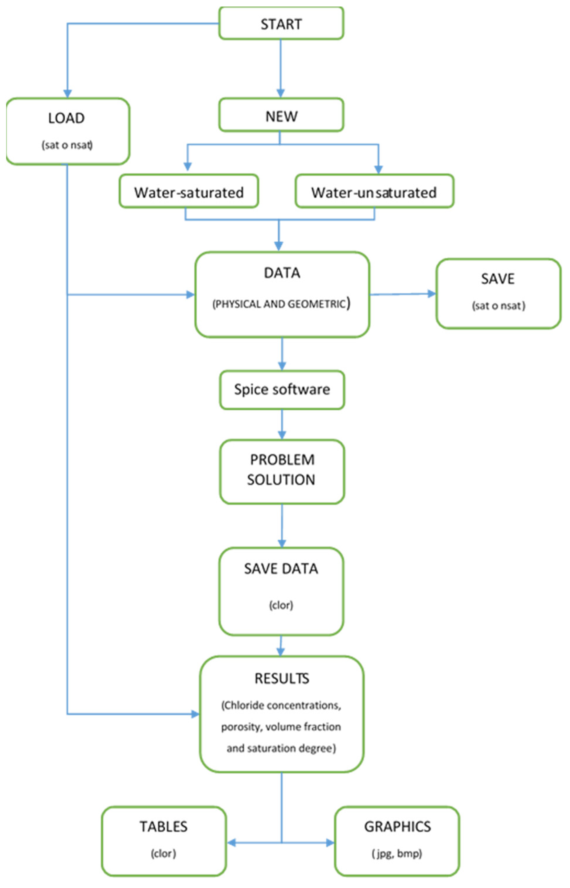
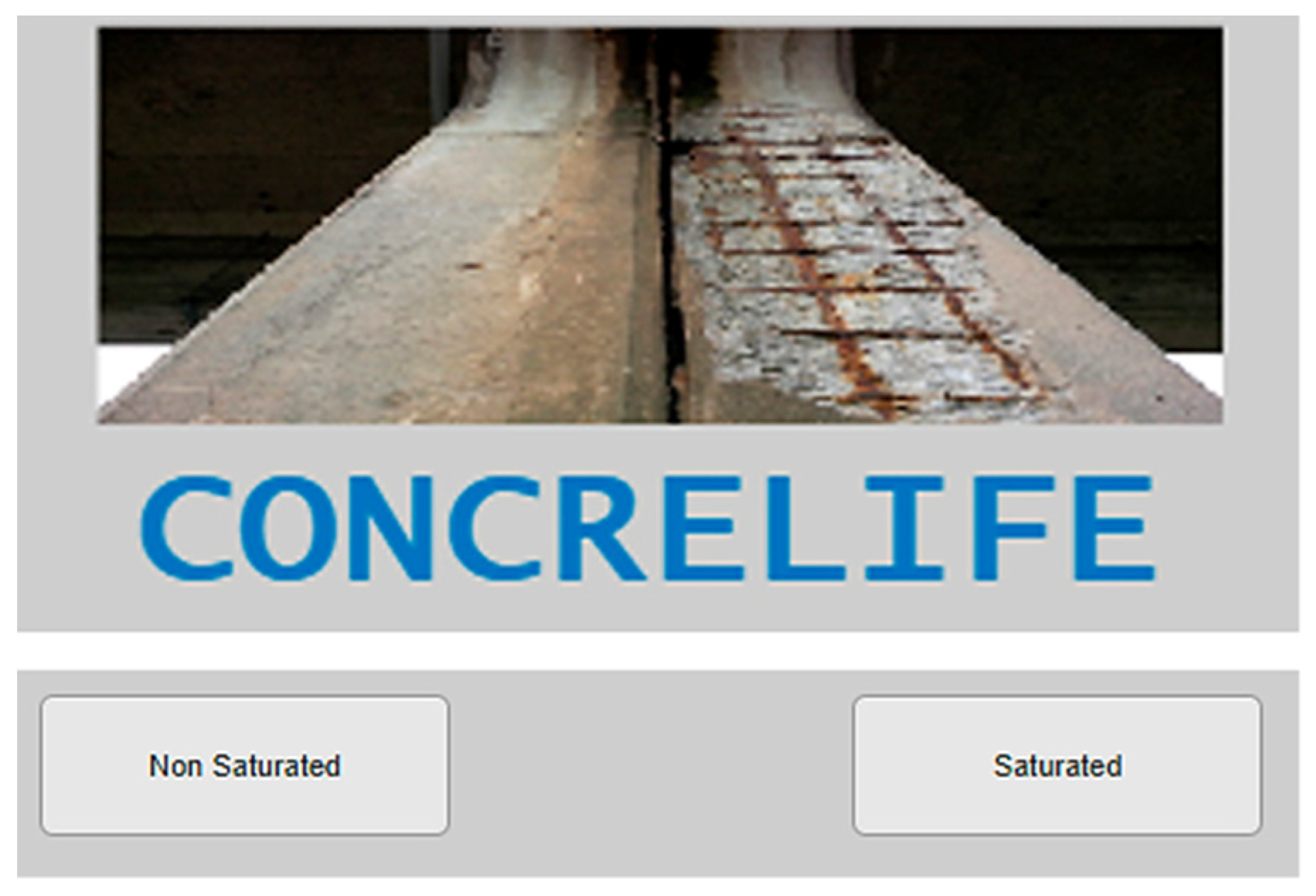
3. The Code Concrelife

The purpose of this software is to obtain numerical solutions to the problem of chloride transport in reinforced concrete, water-saturated or not, under the hypothesis of the existence of bound and precipitated chlorides, taking into account the thermal dependencies of the different coefficients involved in the process. In order to make its design simple and intuitive, a user communication environment has been designed through Windows (for XP, Vista, 7, 8 and 10 operating systems) using Matlab^® [43]. This allows a progressive access to each of the steps necessary for the simulation. The very complete and powerful graphic application of this code is also used to represent the different types of curves of the solution.

The numerical calculation is conducted using models whose designs are based on the Network Simulation Method [8,10] and shown in [44], a tool that takes advantage of the powerful computing algorithms inherent in modern circuit resolution codes [45] to provide practically an exact solution of the model. The errors are relegated to the size of the mesh and are much less than 1%, for relatively low meshes (of the order of 40 or 50 cells in 1-D problems). As the calculation engine for the execution of the models, the free code NgSpice (Spice Code) has been chosen [46]. This software, a circuit simulator with ‘Modified’ BSD license —which is based on three open source software packages Spice3f5, Xspice and Cider1b1—, solves the equations implemented through the circuits created by Concrelife, generating suitable output files with the results obtained.

In summary, the Network Simulation Method consists of transforming the mathematical model that represents the physicochemical problem into a network of electrical circuits. Each cell of the spatial discretisation includes the network model that represents the mathematical model and is connected to adjacent cells or boundary conditions. To convert the mathematical model into a network model, the following steps must be followed: (1) The equivalence between the study variable and the voltage at the central node of the network is established; (2) For this purpose, different electrical devices are available to implement the summand, such as resistors, current generators, batteries, capacitors, etc. and; and (3) The circuit created must comply with Kirchhoff’s laws. The mathematical model described above has been fully implemented in the Concrelife software and no assumptions have been made. A more detailed description of the model can be found in [44].

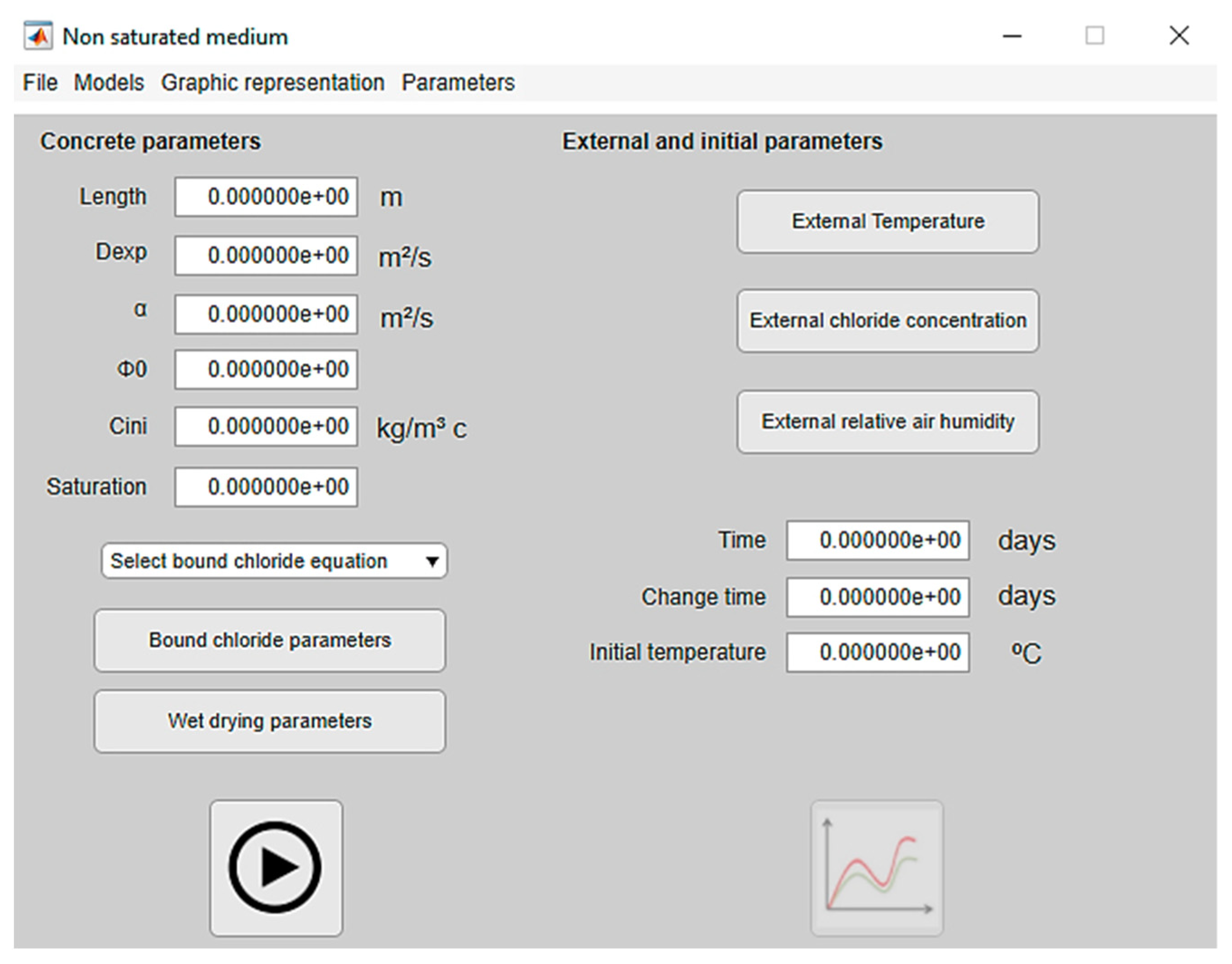
3.1. The Screens of Input Data

The anagram of the program is shown in Figure 3 and its execution follows the scheme represented as a flow chart in Figure 4. The computational solutions are stored to be shown in tabulated form or by graphical representations. For example, instantaneous spatial profiles of the chloride concentration (concentrated in the solution, in the concrete, or bounded and precipitated chloride), temporary distributions of these concentrations in positions selected by the user, total chloride that penetrates the boundary, etc.

Once the program starts, a first communication screen is displayed. As shown in Figure 5, the user selects the type of problem: saturated or unsaturated. According to the choice, the screens in Figure 6 and Figure 7 give access to the problem data entry. For the entire data set, the units in which they are to be expressed are shown.

These screens also display a menu located at the top with four labels. In the first ‘File’ display, the sub-menu of Figure 8a, the user can choose between the following: create a new model, save it once the input data has been entered, load a previously created model, load figures or close the software. The second ‘Models’ display is a submenu to change from the saturated to unsaturated model or vice versa as shown in Figure 8b. The third label, ‘Graphic representation’, allows access to the graphic representation screen as shown in Figure 8c. The last label, ‘Parametrs’, through the only option ‘Calculation parameters’ allows displaying a new window in which the user defines other parameters related to the calculus such as ‘Reltol’ or relative tolerance, to set the compromise between accuracy of results and computing time; ‘Number of division’ to define the number of volume elements or cells; ‘Time interval’ to set the successive times for which boundary conditions change their values; and ‘Number of simulation’ to determine the number of times the results are saved, at regular intervals starting from zero, over the total simulation, Figure 8d.

Going back to the data entry screens, for the saturated problem (Figure 5), the data is organized into three blocks. In the first, left column of the figure, the following data are introduced: length of the domain (‘Lengh’), diffusivity of the chloride in the solution (‘D_exp’), thermal diffusivity (‘α’), the initial porosity (‘ϕ_o’), initial concentration of chloride in the concrete (‘Cl_ini’) and degree of saturation (ϕ_l/ϕ), or ratio between the pore water content and porosity (‘Saturation’). The type of isotherm (‘Select bound chloride equation’) and the parameters that adjusts the corresponding dependence (‘Bound chloride parameters’) complete the data of this column. It is possible to choose between any of the four known isotherms, linear Langmuir (Equation (14a)), non-linear Langmuir (Equation (14b)), non-linear Freundlich (Equation (14c)) and non-linear Langmuir–Freundlich (Equation (14d)), Figure 9a. The parameters involved in each of these dependencies are entered through the screen of Figure 9b that appears clicking ‘Bound chloride parameters’. Note that you can simulate the problem without bound chloride by entering on the linear dependence of Langmuir the value C_b,o = 0.

The second block collects the concentration and temperature of the surrounding fluid (‘External chloride concentration’ and ‘External temperature’, respectively), the total time of simulation (‘Time’), the time interval for which the boundary conditions change (’Change time’) and the initial temperature of the concrete (Initial temperature’). The total time can be split in up to 12 equal intervals allowing the concentration and contour temperature to be changed up to twelve times. Thus, by clicking ‘External chloride concentration’ and ‘External temperature’, the program presents the drop-down in Figure 10a,b, respectively. The concentration and temperature data that applied to the beginning of each time interval are introduced.

In relation to the unsaturated problem (Figure 6), in addition to the above data, the value of the coefficients of the capillary pressure (19) and the diffusion coefficient (20), e, e₁ y A₁, are introduced by clicking the label ‘Wet drying parameters’ in the unsaturated problem screen. This action gives way to the screen of Figure 10c allowing to enter these coefficients whose value depends on whether it is a drying (D) process or a wet (W) process. In addition, clicking the label ‘External relative air humidity’, a new screen in which the table of values of this parameter (between the range [0.001–1]) for the successive time intervals defined above is displayed, Figure 10d.

3.2. Simulation and Graphical Outputs

Once the data has been entered and after clicking the icon , the model is generated by programming in the form of a text file, and NgSpice starts the simulation. This gives way to the presentation of the typical NgSpice software screen [46], where the percentage of time elapsed until complete computing is indicated. An auxiliary screen gives additional information in reference to the simulation number through which the computation progresses, Figure 11.

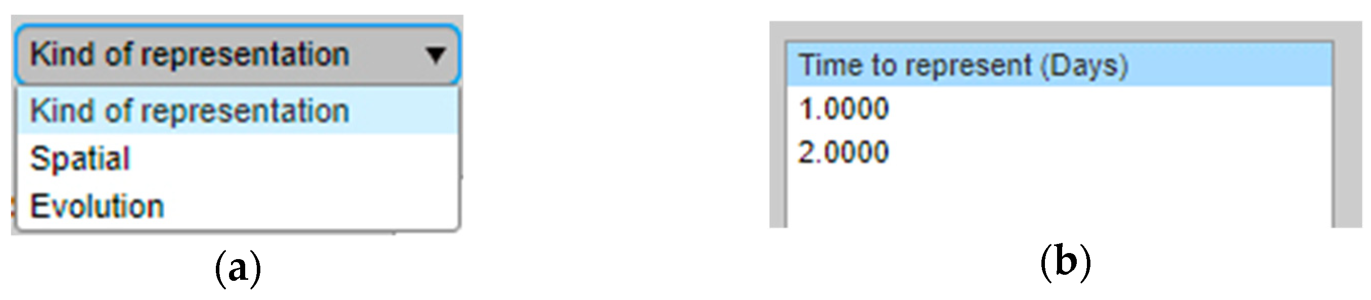
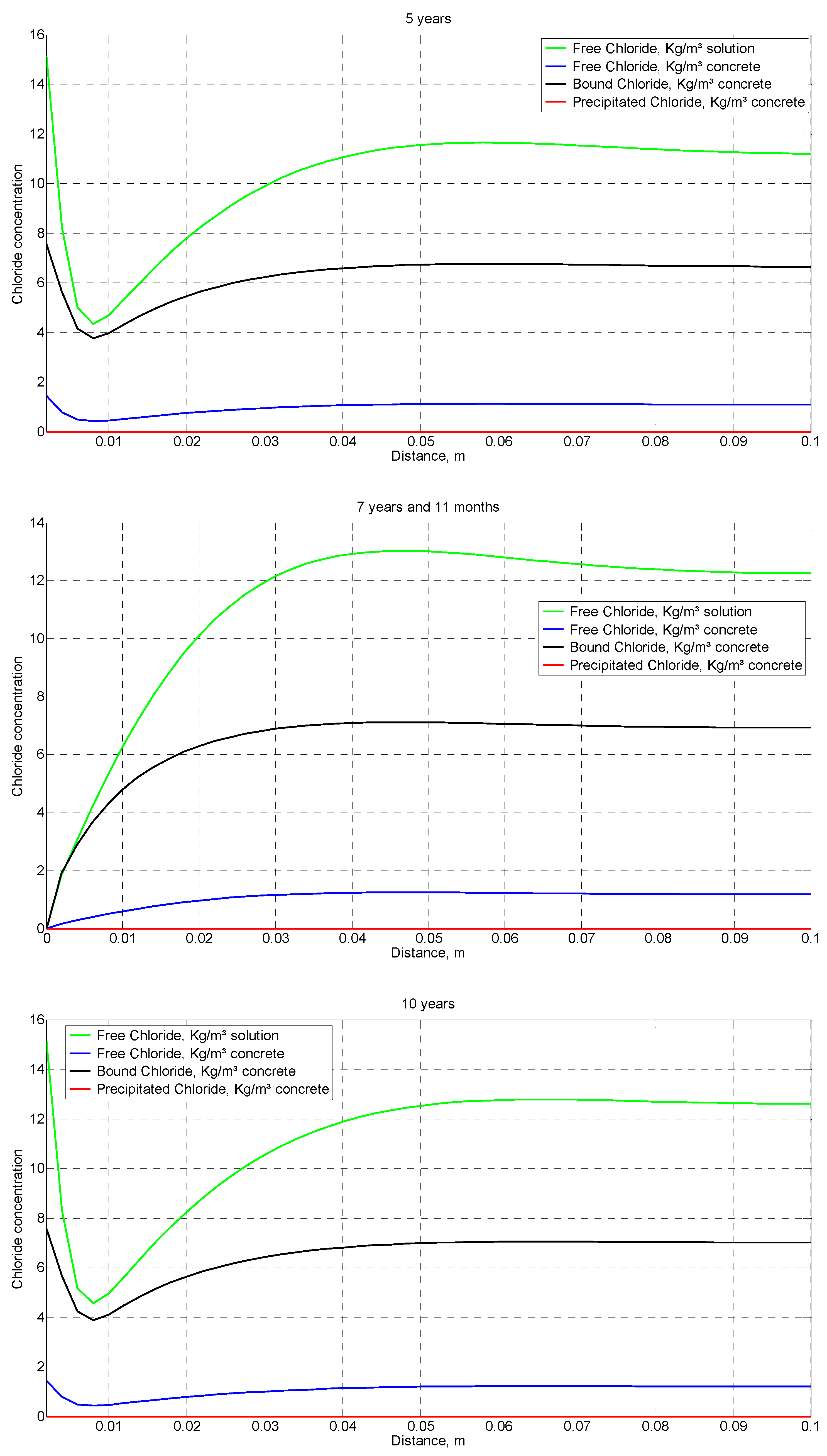
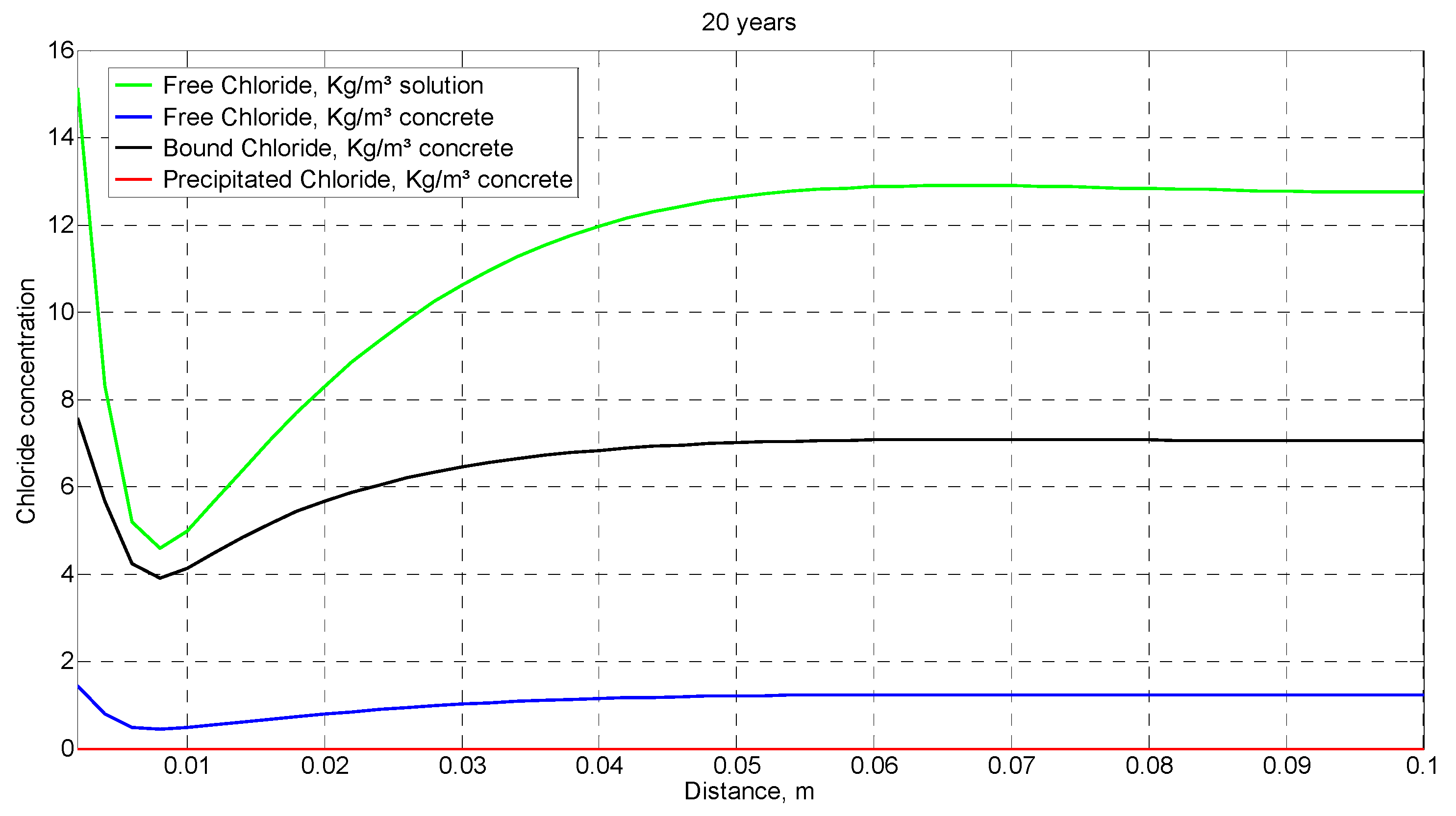
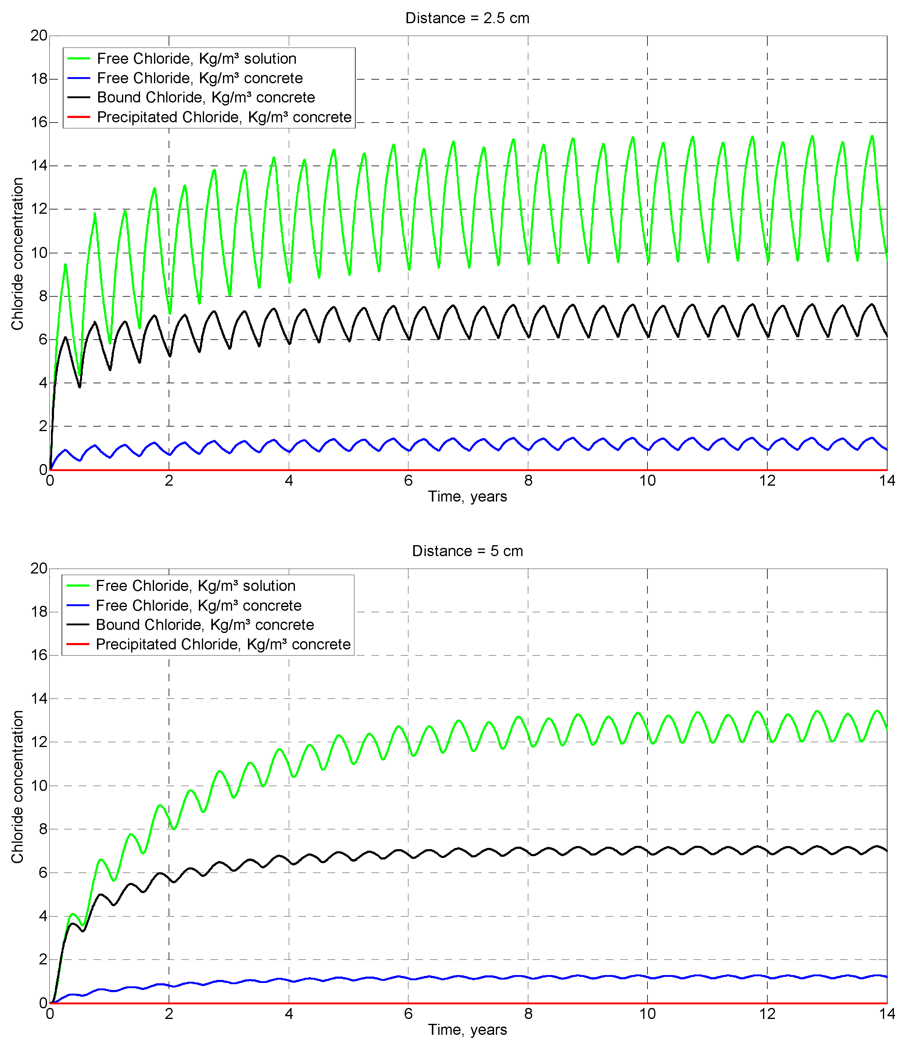
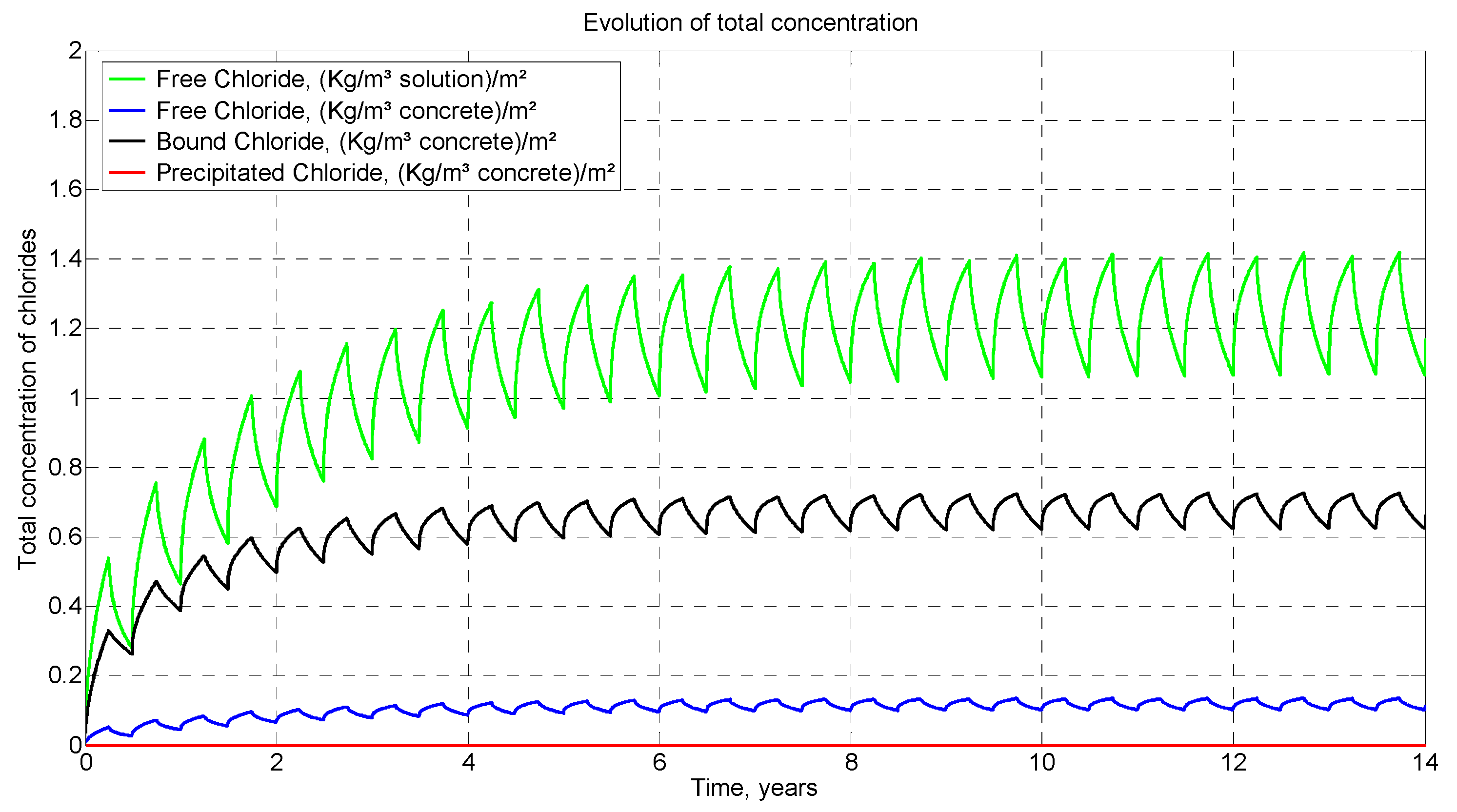
Once the computational calculation is finished, the button accesses the graphical representation of the solutions through the screen of Figure 12. In this, the drop-down ‘Kind of representation’ allows to select between spatial representation of variables (‘Spatial’), in selected moments introduced in the drop-down ‘Time to represent’, and temporal representation of variables (‘Evolution’) at the location chosen in ‘Section to represent’ in the main screen, Figure 13a,b. The variables that can be represented for the saturated problem are (1) free chloride concentration in the solution (kg/m³), ‘Free Chloride concentration (Vol.)’; (2) free chloride concentration in concrete (kg/m³), ‘Free Chloride concentration’; (3) bounded chloride concentration in the concrete (kg/m³), ‘Bound Chloride concentration’; and (4) concrete porosity, ‘Porosity’. For the unsaturated problem, the previous variables plus (5) precipitated chloride concentration in concrete (kg/m³), ‘Precipitated Chloride concentration’; (6) volume fraction of the liquid phase in the pores, ‘Volume fraction of the liquid phase’; and (7) saturation degree, ‘Saturation degree’, Figure 14a,b.

As an illustration, typical representations of Concrelife are shown. The spatial concentration of three species of chlorides after 250 days is shown in Figure 15a. Time evolution of concentration of three species of chloride at 1.2 cm from the boundary is shown in Figure 15b. The free chloride (kg/m³ solution) is represented in the color green, the free chloride (kg/m³ concrete) in blue, and finally, the bound chloride (kg/m³ concrete) in black.

4. Applications

Three applications are presented to demonstrate the efficiency and reliability of Concrelife. For them, a mesh of 50 cells is chosen. Data of the first application, whose purpose is to verify the results of the program are listed in

Table 3. Data of the first application (water-saturated concrete).

Common Parameters
Rg = 8.31 J/mol K	Ea = 19,805 J	Cf,s,sat,(20 °C) = 192 kg/m3	ρps = 2165 kg/m3	ρps = 1892 kg/m3
Co = 18.59 kg/m3 solution for 18 months
φo = 0.134	Dexp = 5.33 × 10−12 m2/s	L = 0.2 m	Ct,i = 0.038 kg/m3 concrete
Bound chloride parameters for Langmuir–Freundlich isotherm
Cbo = 11.895 Kg/m3 concrete			K = 1.1007	α = 0.5639
Temperature parameters
Ta = 20 °C	αT = 7 × 10−7 m2/s
Experimental data [27,47]
Distance (mm)	Free chlorides (kg/m3 concrete)	Bound chlorides (kg/m3 concrete)	Total chlorides (kg/m3 concrete)
6.430	1.8800	7.2694	9.1494
9.495	1.6512	7.0625	8.7137
12.160	1.4421	6.8359	8.2780
14.580	1.2439	6.5984	7.8423

. The experimental data have been taken from the experimental tests conducted by [27,47], where the latter author [27] indicates that the first two experimental data have been ignored, since it seemed that the bound chloride ions were more soluble in positions close to the surface. One possible explanation is that the standard measurement method for measuring free chloride is less accurate at high concentrations. Table 3 shows results obtained by [27,47] ignoring these first two data, as indicated by [27]. The coefficients of the Langmuir–Freundlich nonlinear isotherm chosen to approximate the C_b-C_f,c dependence have been adjusted using the spreadsheet [27,47]. Figure 16 shows the concentrations of free, bound and total chlorides, given by Concrelife, in typical locations of a concrete sample after 18 months. Note that the concentration level of free chloride C_f,c exceeds the threshold of this variable (0.6–1.2 kg/m³ of concrete) for which armor corrosion begins [2,3,26,48,49]. After integrating the C_f,c concentration profile obtained in the simulation along each of the slices in which the sample was cut in the experimental test, we can compare the experimental results and those of the simulation using Concrelife.

Table 4. Deviations between experimental and numerical solutions.

Distance (mm)	Free Chlorides (kg/m3 Concrete)		Bound Chlorides (kg/m3 Concrete)		Total Chlorides (kg/m3 Concrete)
	Experimental	Simulation	Experimental	Simulation	Experimental	Simulation
6.430	1.8800	1.9140 (1.807%)	7.2694	7.2508 (0.256%)	9.1494	9.1648 (0.168%)
9.495	1.6512	1.6638 (0.765%)	7.0625	7.0423 (0.286%)	8.7137	8.7062 (0.087%)
12.160	1.4421	1.4571 (1.041%)	6.8359	6.8296 (0.092%)	8.2780	8.2867 (0.105%)
14.580	1.2439	1.2804 (2.936%)	6.5984	6.6072 (0.133%)	7.8423	7.8876 (0.577%)

collects this comparison and verifies that the deviations between experimental and numerical solutions are minimal, with relative errors below 2.94%.

The second application, whose data are listed in

Table 5. Saturated problem. Data of the second application.

Common Parameters
Rg = 8.31 J/mol K	Ea = 19,805 J		Cf,s,sat,(20 °C) = 192 kg/m3	ρps = 2165 kg/m3	ρps = 1892 kg/m3
Co = 19.455 kg/m3 solution for 0 ≤ t ≤ 5 years				Co = 1 kg/m3 solution for t > 5 years
φo = 0.1	Dexp = 9.35 × 10−11 m2/s		L = 0.2 m	Cf,s,i = 0 kg/m3
Bound chloride parameters for Langmuir–Freundlich isotherm
Cbo = 12.5366 Kg/m3 concrete				K = 0.6934	α = 0.9451
Temperature parameters
Ta = 10 °C			αT = 7 × 10−7 m2/s
External temperature
Month	${\mathrm{T}}_{\left({\mathrm{S}}_{\mathrm{ext},\mathrm{iso}}\right)}$ (°C)	Month	${\mathrm{T}}_{\left({\mathrm{S}}_{\mathrm{ext},\mathrm{iso}}\right)}$ (°C)	Month	${\mathrm{T}}_{\left({\mathrm{S}}_{\mathrm{ext},\mathrm{iso}}\right)}$ (°C)
1	10	5	15	9	18
2	11	6	17	10	17
3	11	7	18	11	15
4	13	8	19	12	11

, is a coupled problem in a saturate concrete sample, where to show the possibilities of changing the boundary conditions in the software, it is proposed that the external chloride concentration drops sharply after 5 years while temperature boundary conditions simulate approximately those of an annual seasonal cycle. This could be the case of a structure submerged in a swimming pool that is initially filled with seawater and after 5 years is changed to water with a lower salt concentration. To approximate the dependence between bound and free chlorides, the Langmuir–Freundlich isotherm with typical values for its coefficients has been chosen. The surface of the concrete opposite to that subjected to the outside environment (x = l_o) has been considered adiabatic for heat flux and impermeable for the chloride ions. This is a suitable option since the geometry of the problem is symmetric in general allowing to simulate only half of the domain. The simulation time chosen is sufficient to ensure that the concentration of free chloride in the supposed position of the reinforcement bar is near or exceeds the threshold of corrosion initiation. This time is far from the characteristic time of the process, l_o²/D_exp.

The simulation results are shown in Figure 17, Figure 18 and Figure 19. In the first, concentration profiles for C_f,s (free chloride in kg/m³ solution), C_f,c (free chloride in kg/m³ concrete) and C_b (bound chloride in kg/m³ solution) at 5 and 20 years are depicted. The change in profile caused by the fall in concentration at the boundary (x = 0) as well as the delay in this fall as we enter inside the sample are appreciated. The time dependent concentration of the same chlorides at typical locations, x = 5 and 10 cm are depicted in Figure 18. Finally, Figure 19 shows the total chloride quantity of C_f,s, C_b and C_f,c that crosses the boundary between 0 and t days. It is immediate to deduce from these graphs the time for which the concentration threshold of C_f,c that starts the corrosion of the reinforcement in each position is reached.

The third application refers to an unsaturated problem whose data lists in

Table 6. Unsaturated problem. Data of the third application.

Common Parameters
Rg = 8.31 J/mol K	Ea = 19,805 J		Cf,s,sat,(20 °C) = 192 kg/m3	ρps = 2165 kg/m3	ρps= 1892 kg/m3
φo = 0.1	Dexp = 8.30 × 10−11 m2/s		L = 0.1 m	Sat = 1
Bound chloride parameters for Langmuir–Freundlich isotherm
Cbo = 13.7835 Kg/m3 concrete				K = 0.8662	α = 0.9068
Parameters for diffusion coefficient and permeability
e = 0.5331 (wet cycle)	e = 0.5331 (drying cycle)		ko = 2.45 × 10−21 m2
Parameters for capillary pressure
${\mathsf{\rho }}_1$ = 0.1 MPa (wet cycle)	${\mathsf{\rho }}_1$ = 0.1 MPa (drying cycle)			a1 = 3 (wet cycle)	a1 = 7 (drying cycle)
Concentration parameters
Cf,s,i = 0 kg/m3
External concentration
Month	Co (kg/m3 solution)	Month	Co (kg/m3 solution)	Month	Co (kg/m3 solution)
1	19.455	5	1.822 × 10−8	9	19.455
2	19.455	6	1.822 × 10−8	10	1.822 × 10−8
3	19.455	7	19.455	11	1.822 × 10−8
4	1.822 × 10−8	8	19.455	12	1.822 × 10−8
Temperature parameters
Ta = 10 °C		αT = 7 × 10−7 m2/s
External temperature
Month	${\mathrm{T}}_{\left({\mathrm{S}}_{\mathrm{ext},\mathrm{iso}}\right)}$ (°C)	Month	${\mathrm{T}}_{\left({\mathrm{S}}_{\mathrm{ext},\mathrm{iso}}\right)}$ (°C)	Month	${\mathrm{T}}_{\left({\mathrm{S}}_{\mathrm{ext},\mathrm{iso}}\right)}$ (°C)
1	10	5	15	9	18
2	11	6	17	10	17
3	11	7	18	11	15
4	13	8	19	12	11
Relative humidity parameters
External relative humidity
Month	hr	Month	hr	Month	hr
1	1	5	0.3	9	1
2	1	6	0.7	10	0.5
3	1	7	1	11	0.4
4	0.4	8	1	12	0.6

. In this example, the external temperature has a slow harmonic variation throughout the year. For the concentration of chloride in the surrounding atmosphere, the cycle of variation is 0.5 years with a square waveform, showing a structure submerged in seawater some months and not others. Relative humidity values throughout the year have been chosen arbitrarily from those possible for this example, reproducing an almost harmonic function of 0.5-year cycle, thus showing the ability to change the boundary conditions of the software. Finally, the relative humidity value equal to unity means that the structure is submerged.

The simulation results are shown in Figure 20, Figure 21 and Figure 22. The concentration of C_f,s (free chloride in kg/m³ solution), C_f,c (free chloride in kg/m³ concrete) and C_b (bound chloride in kg/m³ solution) along the concrete at times 1, 5, 7.9, 10 and 20 years, Figure 20, clearly show the effect on these profiles of the seasonal dependence of the concentration of the surrounding atmosphere, clearly showing the effect of the structure being submerged some months and not others. This influence results in the temporary harmonic variation of the concentration at points inside the concrete being delayed the further we move away from the outer surface of the sample. Thus, in the months when the structure is not submerged, the chlorides already in the structure can diffuse both into the structure and to the near-surface areas. Similar results have been obtained in real structures subjected to a seasonal tidal cycle [50]. Figure 21 shows the time dependent concentration of bounded and free chlorides at typical locations, x = 2.5, 5 and 7.5 cm. These distributions, as expected, show a first transition of approximately 9 years for the indicated positions, after which the concentrations remain harmonic without average variation. Finally, the total chloride that enters the concrete from the initial moment until t days, separated in its components C_f,s, C_b and C_f,c, is shown in Figure 22.

5. Final Comments and Conclusions

The proposed applications allow us to state that the Concrelife software, designed for the simulation of the problem of penetration of chlorides in reinforced concrete, saturated or not, reproduces the most demanding conditions to this problem and thus reports reliable results that allow defining the first state of the useful life of a structure, the period of time that elapses from the start-up of the structure until the beginning of the reinforcement corrosion. The program assumes the current empirical dependencies on the parameters involved (density and viscosity of the solution, diffusivity of the chloride) with the temperature. The temperature field is also obtained numerically from the solution of the non-coupled thermal problem, which allows the implementation of time-dependent boundary conditions. Regarding the penetration of chlorides, the software incorporates the generation of bound chloride and precipitated chloride, phenomena that lead to a change in the porosity of concrete thanks to the formation of Friedel´s salt and precipitate crystals. All known types of empirical dependencies between bounded and free chloride (linear Langmuir, non-linear Langmuir, Freundlich and Langmuir-Freundlich) have been incorporated into the program. In addition, the software allows the introduction of time dependence boundary conditions, in the form of piece-wise functions, for the chloride concentration and relative humidity.

The need to simulate long-term time intervals (usually years), which inevitably entails large computing times and a huge amount of resulting data whose processing is not available to personal computers, has been circumvented with the execution of successive temporary windows (up to 12) of which the final data is retained, thus avoiding saturation of the computer memory. The graphical output environment of the software, based on Matlab ^® [43], incorporates the presentation of the spatial and temporal dependences of all the variables of interest such as, (1) the spatial distribution of all species of chloride in set times, (2) the temporal evolution of the concentrations in each position of the domain, (3) the total time dependent chloride that penetrates through the boundary, (4) the porosity, and (5) the water content in the pores.

To facilitate the handling by users unfamiliar with numerical techniques and other aspects of computing, the communication environment with the program’s user is conducted through windows for both data entry, computation start and graphical representation of results. Its versatility allows the execution of any type of problem in 1-D rectangular geometry (which are the most common cases) that can be presented in reinforced concrete columns including changes in relative humidity, wet-drying, column washing, etc.

The numerical technique that Concrelife software applies is based on the network method, a tool verified in many other problems of similar or greater complexity to those presented in this work. The software incorporates standard network models for the most complex scenarios to which, after the association of specific values with the elements that integrate these models, it executes them in the free code NgSpice [46] taking advantage of the modern and powerful computing algorithms that it incorporates. The result of the simulation is, in practice, the exact solution of the model, leaving the errors relegated to the size of the mesh chosen—in general, less than 0.5% for relatively small meshes.

References

1. Saetta, A.V.; Scotta, R.V.; Vitaliani, R.V. Analysis of chloride diffusion into partially saturated concrete. ACI Mater. J. 1993, 90, 441–451. [Google Scholar]
2. Liu, Y. Modeling the Time-to-Corrosion Cracking of the Cover Concrete in Chloride Contaminated Reinforced Concrete Structures. Ph.D. Thesis, Virginia Polytechnic Institute and State University, Blacksburg, VA, USA, 1996. [Google Scholar]
3. Liu, Y.; Weyers, R.E. Modeling the time to corrosion cracking in chloride contaminated reinforced concrete structures. ACI Mater. J. 1998, 95, 675–681. [Google Scholar]
4. Guzman-Gutiérrez, S. Modelzación del Deterioro de Tableros de Puentes de Hormigón por Difusión de Cloruros y Corrosión de la Armadura Pasiva. Ph.D. Thesis, ETS de Ing. de Caminos Canales y Puertos, Madrid, Spain, 2010. [Google Scholar]
5. Liang, M.T.; Huang, R.; Jheng, H.Y. Reconsideration for a study of the effect of the chloride binding on service life predictions. J. Mar. Sci. Technol. 2011, 19, 531–540. [Google Scholar] [CrossRef]
6. Andrade, C.; Climent, M.A.; de Vera, G. Procedure for calculating the chloride diffusion coefficient and Surface concentration from a profile having a maximum beyong the concrete Surface. Mater. Struct. 2015, 48, 863–869. [Google Scholar] [CrossRef]
7. Sanchez-Perez, J.F.; Hidalgo, P.; Alhama, I. Concrelife. Cementos la Cruz. Registration Requested on October 1, 2019. Nº 08/2019/743 [Software]. 2019. [Google Scholar]
8. Horno, J.; García-Hernández, M.T.; González-Fernández, C.F. Digital simulation of electrochemical processes by the network approach. J. Electroanal. Chem. 1993, 352, 83–97. [Google Scholar] [CrossRef]
9. González Fernández, C.F.; Alhama, F.; Horno, J.; López García, J.J. Network Simulation Method; Montijano, J.H., Ed.; Research Signpost: Trvandrum, India, 2003. [Google Scholar]
10. Sánchez-Pérez, J.F.; Marín, F.; Morales, J.L.; Cánovas, M.; Alhama, F. Modeling and simulation of different and representative engineering problems using Network Simulation Method. PLoS ONE 2018, 13, e0193828. [Google Scholar] [CrossRef] [Green Version]
11. Alhama, I.; Soto, A. FATSIM-A: Fluid Flow and Solute Transport Simulator. Universidad Politécnica de Cartagena. Nº Mu-1093-2010 [Software]. 2010. [Google Scholar]
12. Sanchez-Perez, J.F.; Alhama, I.; García-Ros, G. SICOMED_3D (Simulación de consolidación con mechas drenantes). Universidad Politécnica de Cartagena. Registration requested on 28 November 2016. Nº 08/2017/196 [software]. 2016. [Google Scholar]
13. Alhama, F.; Alhama, I.; Sanchez-Perez, J.F.; Morales-Guerrrero, J.L. CODENS_13 (Coupled Ordinary Differencial Equations by Network Simulation). Universidad Politécnica de Cartagena. Registration Requested on 16 January 2014. Nº 08/2014/56 [Software]. 2014. [Google Scholar]
14. Sanchez-Perez, J.F.; Moreno, J.A.; Alhama, F. OXIPSIS_12 (Oxidation Processes Simulation Software). Universidad Politécnica de Cartagena. Registration requested on 13 July, 2013. Nº 08/2013/616 [software]. 2013. [Google Scholar]
15. Alhama, I.; Soto, A.; Alhama, F. FATSIM-A: An educational tool based on electrical analogy and the code PSPICE to simulate fluid flow and solute transport processes. Comput. Appl. Eng. Educ. 2011, 16, 72–84. [Google Scholar]
16. Sánchez-Pérez, J.F.; Alhama, F.; Moreno, J.A. An efficient and reliable model based on network method to simulate CO2 corrosion with protective iron carbonate films. Comput. Chem. Eng. 2012, 39, 57–64. [Google Scholar] [CrossRef]
17. Sánchez-Pérez, J.F.; Moreno, J.A.; Alhama, F. Numerical Simulation of High-Temperature Oxidation of Lubricants Using the Network Method. Chem. Eng. Commun. 2015, 202, 982–991. [Google Scholar] [CrossRef]
18. Sánchez-Pérez, J.F.; Conesa, M.; Alhama, I. Solving ordinary differential equations by electrical analogy: A multidisciplinary teaching tool. Eur. J. Phys. 2016, 37, 065703. [Google Scholar] [CrossRef]
19. Alhama, I.; García-Ros, G.; Alhama, F. Universal solution for the characteristic time and the degree of settlement in nonlinear soil consolidation scenarios. A deduction based on nondimensionalization. Commun. Nonlinear Sci. Numer. Simular. 2018, 57, 186–201. [Google Scholar] [CrossRef]
20. Sánchez-Pérez, J.F.; Alhama, F.; Moreno, J.A.; Canovas, M. Study of main parameters affecting pitting corrosion in a basic medium using the network method. Results Phys. 2019, 12, 1015–1025. [Google Scholar] [CrossRef]
21. Martín-Pérez, B.; Zibara, H.; Hooton, R.D.; Thomas, M.D. A study of the effect of chloride binding on service life predictions. Cem. Concr. Res. 2000, 30, 1215–1223. [Google Scholar] [CrossRef]
22. Martín-Pérez, B.; Pantazopoulou, S.J.; Thomas, M.D.A. Numerical solution of mass transport equations in concree sructures. Comput. Struct. 2001, 79, 1251–1264. [Google Scholar] [CrossRef] [Green Version]
23. Meijers, S.J.H.; Bijen, J.M.; de Borst, R.; Fraaij, A.L.A. Computational results of a model for chloride ingress in concrete including convection, dry-wetting cycles and carbonatation. Mater. Struct. 2005, 38, 145–154. [Google Scholar] [CrossRef]
24. Garcés, P.; Saura, P.; Mendez, A.; Zornoza, E.; Andrade, C. Effect of nitrite in corrosion of reinforcing steel in neutral and acid solutions simulating the electrolytic environments of micropores of concrete in the propagation period. Corros. Sci. 2008, 50, 498–509. [Google Scholar] [CrossRef]
25. Iqbal, P.O.; Ishida, T. Modelling of chloride transport coupled with enhanced moisture coductivity in concrete exposed to marine environment. Cem. Concr. Res. 2009, 39, 329–339. [Google Scholar] [CrossRef]
26. Solano-Rodríguez, S.A.; Estupiñán-Durán, H.A.; Vásquez-Quintero, C.; Peña-Ballesteros, D.Y. Simulation of ion cl- diffusion until depassivation of reinforcing steel in concrete with microsilica as additive and exposed to carbonation. Boletín Ciencias de la Tierra 2013, 34, 15–24. [Google Scholar]
27. Fenaux, M. Modelling of Chloride Transport in Non-Saturated Concrete. From Microscale to Macroscale. Ph.D. Thesis, ETS de Ing. de Caminos Canales y Puertos, Madrid, Spain, 2013. [Google Scholar]
28. Gálvez, J.C.; Guzmán, S.; Sancho, J.M. Cover cracking of the reinforced concrete due to rebar corrosion induced by chloride penetration. In Proceedings of the 8th International Conference on Fracture Mechanics of Concrete and Concrete Structures (FraMCoS), Toledo, Spain, 10–14 March 2014. [Google Scholar]
29. Lehner, P.; Konecny, P.; Ghosh, P.; Tran, Q. Numerical analysis of chloride diffusion considering time-dependent diffusion coefficient. Int. J. Math. Comput. Simul. 2014, 8, 102–106. [Google Scholar]
30. EN 12390-11:2015. Testing Hardened Concrete. Determination of the Chloride Resistance of Concrete, Unidirectional Diffusion. Available online: https://www.une.org/ (accessed on 13 September 2019).
31. Marchand, J.; Gerard, B.; Delagrave, A. Ion transport mechanisms in cement-based materials. In Material Science of Concrete; American Ceramic Society: Westerville, OH, USA, 1998; Volume 5, pp. 307–400. [Google Scholar]
32. Jensen, O.M.; Hansen, P.F.; Coats, A.M.; Glasser, F.P. Chloride ingress in cement paste and mortar. Cem. Concr. Res. 1999, 29, 1497–1504. [Google Scholar] [CrossRef]
33. Jooss, M.; Reinhardt, H.W. Permeability of diffusivity of concrete as function of temperature. Cem. Res. Concr. 2002, 32, 1497–1504. [Google Scholar] [CrossRef]
34. Seidell, A. Solubilities of Inorganic and Metal Organic Compounds, Volume 1; D. Van Nostrand Company Inc.: New York, NY, USA, 1940. [Google Scholar]
35. McCutcheon, S.C.; Martin, J.L.; Barnwell, T.O. Water Quality. In Handbook of Hydrology; Maidment, D.D., Ed.; McGraw-Hill: New York, NY, USA, 1993. [Google Scholar]
36. Boufadel, M.C.; Suidan, M.T.; Venosa, A.D. A numerical model for density-and-viscosity-dependent flows in two-dimensional variably satured porous media. J. Contam. Hydrol. 1999, 37, 1–20. [Google Scholar] [CrossRef]
37. Samson, E.; Marchand, J. Modeling the effect of temperature on ionic transport in cementittious material. Cem. Concr. Res. 2007, 37, 455–468. [Google Scholar] [CrossRef]
38. Guimarăes, A.T.C.; Climent, M.A.; de Vera, G.; Vicente, F.J.; Rodrigues, F.T.; Andrade, C. Determination of chloride difussivity through partially saturated Portland cement concrete by a simplified procedure. Constr. Build. Mater. 2011, 25, 785–790. [Google Scholar] [CrossRef]
39. Pradelle, S.; Thiery, M.; Véronique-Baroghel, B. Comparison of existing chloride ingress models within concretes exposed to seawater. Mater. Struct. 2016, 49, 4497–4516. [Google Scholar] [CrossRef]
40. Van Genuchten, M.T. A closed-form equation for predicting the hydraulic conductivity of unsaturared soils. Soil Sci. Soc. Am. 1980, 44, 892–898. [Google Scholar] [CrossRef] [Green Version]
41. Kestin, J.; Khalifa, H.E.; Correia, R.J. figures of dynamic and kinematic viscosity of aqueous NaCl solutions in the temperature range 20–150 °C and pressure range 0.1–35 MPa. J. Phys. Chem. Ref. Data 1983, 10, 817–820. [Google Scholar]
42. Brooks, R.H.; Corey, A.T. Properties of porous media affecting fluid flow. Irrigation and drainage division. Proc. Am. Soc. Civ. Eng. 1966, 92, 61–88. [Google Scholar]
43. Matlab Software® [on line]. (Quoted 2019). Available online: https://es.mathworks.com/products/matlab.html (accessed on 4 November 2022).
44. Hidalgo, P. Modelización y Simulación del Transporte de Cloruros en Estructuras de Hormigón Armado para Ambientes Marinos. Ph.D. Thesis, Universidad Politécnica de Cartagena (UPCT), Cartagena, España, 2020. [Google Scholar]
45. Nagel, L.W. SPICE2: A Computer Program to Simulate Semiconductor Circuits; University of California Berkeley: Berkeley, CA, USA, 1975. [Google Scholar]
46. NgSpice Software [on line]. (Quoted 2019). Available online: http://ngspice.sourceforge.net/index.html (accessed on 4 November 2022).
47. Abdelkader, M. Influencia de la Composición de Distintos Hormigones en los Mecanismos de Transporte de Iones Agresivos Procedentes de Medios Marinos. Ph.D. Thesis, ETS de Ing. de Caminos Canales y Puertos, Madrid, Spain, 2010. [Google Scholar]
48. Comité Euro-International d’Beton. Draft CEB Guide to Durable Concrete Structures. Bull. D'inform. 1985, 166. Available online: https://www.fib-international.org/publications/ceb-bulletins/draft-ceb-guide-to-durable-concrete-structures-detail.html (accessed on 4 November 2022).
49. RILEM Committee 60-CSG, Corrosion of Steel in Concrete, State of Art Report; Schiessl, P. (Ed.) Chapman and Hall: London, UK, 1987. [Google Scholar]
50. Andrade, C.; Prieto, M.; Tanner, P.; Tavares, F.; d’Andrea, R. Testing and modelling chloride penetration into concrete. Constr. Build. Mater. 2013, 39, 9–18. [Google Scholar] [CrossRef]
51. CDTI. Centro para el Desarrollo Tecnológico Industrial. Ministry of Science and Competitiveness (Spain). Equipo para la determinación de la vida útil de las estructuras de hormigón armado—Concrelife. Funding Reference Number IDI-20170080. 2017. [Google Scholar]
52. Cementos la Cruz [on line]. (Quoted 2019). Available online: https://www.cementoscruz.com/ (accessed on 4 November 2022).
53. Universidad Politécnica de Cartagena (UPCT). Unidad de Investigación y Transferencia Tecnologica (UITT) [on line]. (Quoted 2019). Available online: https://www.upct.es/uitt/es/inicio/ (accessed on 4 November 2022).
Figure 1. Geometry and boundary conditions for the problem of water-saturated concrete. Nomenclature: Cf,s is the free chloride concentration in the solution (kg/m3 solution), Cf,s,i is the initial free chloride concentration in the solution (kg/m3 solution), Co is the free chloride concentration at the surrounding liquid (kg/m3 solution), L is the concrete structure length (m), Ta is the initial temperature (°C), T ( S ext , iso ) is the external temperature (°C), x is the position (m) and ϕo is the initial porosity (m3 of pores/m3 of concrete).
Mathematics 10 04810 g001
Figure 2. Geometry and boundary conditions for the problem of water-unsaturated concrete. Nomenclature: Cf,s is the free chloride concentration in the solution (kg/m3 solution), Cf,s,i is the initial free chloride concentration in the solution (kg/m3 solution), Co is the free chloride concentration at the surrounding liquid (kg/m3 solution), hr is the relative humidity of the surrounding atmosphere, L is the concrete structure length (m), Ta is the initial temperature (°C), T ( S ext , iso ) is the external temperature (°C), x is the position (m), ϕo is the initial porosity (m3 of pores/m3 of concrete) and ϕ l , o is the initial pore water content.
Mathematics 10 04810 g002
Figure 3. Anagram of Concrelife.
Mathematics 10 04810 g003
Figure 4. Flow diagram of Concrelife software.
Mathematics 10 04810 g004
Figure 5. Screen to select the type of problem.
Mathematics 10 04810 g005
Figure 6. Screen of input data for saturated problem.
Mathematics 10 04810 g006
Figure 7. Screen of input data for unsaturated problem.
Mathematics 10 04810 g007
Figure 8. (a) File management submenu, (b) Access to model change, (c) Access to graphic representations, (d) Calculation parameter window.
Mathematics 10 04810 g008
Figure 9. (a) Screen to choose the type of isotherm, (b) Screen for the introduction of the isotherm´s coefficients.
Mathematics 10 04810 g009
Figure 10. Window for introducing: (a) the list of free chloride concentrations at the boundary, (b) the list of temperature at the boundary, (c) the parameters related to capillary pressure and diffusion coefficient, (d) the relative humidity table.
Mathematics 10 04810 g010
Figure 11. Auxiliary screen to show the simulation number in process (the eighth day of the 365 planned).
Mathematics 10 04810 g011
Figure 12. Screen to accesses the graphical solutions.
Mathematics 10 04810 g012
Figure 13. Drop down to select, (a) The type of representation, (b) the time for the spatial representation.
Mathematics 10 04810 g013
Figure 14. Variables to be shown. (a) saturated, (b) unsaturated.
Mathematics 10 04810 g014
Figure 15. (a) Spatial concentration of three species of chloride, Cf,s (free chloride in kg/m3 solution), Cf,c (free chloride in kg/m3 concrete) and Cb (bound chloride in kg/m3 solution), after 250 days. (b) Time dependence of concentration of three species of chloride at x = 1.2 cm.
Mathematics 10 04810 g015
Figure 16. Experimental and Concrelife concentration profiles.
Mathematics 10 04810 g016
Figure 17. Concentration profiles of Cf,s (free chloride in kg/m3 solution), Cf,c (free chloride in kg/m3 concrete) and Cb (bound chloride in kg/m3 solution), at (a) 5 and (b) 20 years.
Mathematics 10 04810 g017
Figure 18. Time dependent concentration of Cf,s (free chloride in kg/m3 solution), Cf,c (free chloride in kg/m3 concrete) and Cb (bound chloride in kg/m3 solution) at (a) x = 5 and (b) 10 cm.
Mathematics 10 04810 g018
Figure 19. Time dependent of total chloride of Cf,s (free chloride in kg/m3 solution), Cf,c (free chloride in kg/m3 concrete) and Cb (bound chloride in kg/m3 solution) that penetrates the boundary.
Mathematics 10 04810 g019
Figure 20. Spatial concentration of Cf,s (free chloride in kg/m3 solution), Cf,c (free chloride in kg/m3 concrete), Cb (bound chloride in kg/m3 solution) and Cp (precipitated chloride in kg/m3 concrete) after 1, 5, 7.9, 10 and 20 years.
Mathematics 10 04810 g020aMathematics 10 04810 g020bMathematics 10 04810 g020c
Figure 21. Time dependent concentration of Cf,s (free chloride in kg/m3 solution), Cf,c (free chloride in kg/m3 concrete), Cb (bound chloride in kg/m3 solution) and Cp (precipitated chloride in kg/m3 concrete) at x = 2.5, 5 and 7.5 cm.
Mathematics 10 04810 g021aMathematics 10 04810 g021b
Figure 22. Time dependent of total chloride of Cf,s (free chloride in kg/m3 solution), Cf,c (free chloride in kg/m3 concrete), Cb (bound chloride in kg/m3 solution) and Cp (precipitated chloride in kg/m3 concrete) that penetrates the boundary.
Mathematics 10 04810 g022