Article

A Lagrange Programming Neural Network Approach with an 0-Norm Sparsity Measurement for Sparse Recovery and Its Circuit Realization

1
College of Electronics and Information Engineering, Shenzhen University, Shenzhen 518060, China
2
Department of Electrical Engineering, City University of Hong Kong, Hong Kong
3
Department of Electrical and Electronic Engineering, Imperial College, London SW7 2BX, UK
*
Author to whom correspondence should be addressed.
Mathematics 2022, 10(24), 4801; https://doi.org/10.3390/math10244801
Submission received: 25 November 2022 / Revised: 12 December 2022 / Accepted: 13 December 2022 / Published: 16 December 2022
(This article belongs to the Special Issue Mathematics and Its Applications in Science and Engineering II)

Abstract

:
Many analog neural network approaches for sparse recovery were based on using 1 -norm as the surrogate of 0 -norm. This paper proposes an analog neural network model, namely the Lagrange programming neural network with p objective and quadratic constraint (LPNN-LPQC), with an 0 -norm sparsity measurement for solving the constrained basis pursuit denoise (CBPDN) problem. As the 0 -norm is non-differentiable, we first use a differentiable p -norm-like function to approximate the 0 -norm. However, this p -norm-like function does not have an explicit expression and, thus, we use the locally competitive algorithm (LCA) concept to handle the nonexistence of the explicit expression. With the LCA approach, the dynamics are defined by the internal state vector. In the proposed model, the thresholding elements are not conventional analog elements in analog optimization. This paper also proposes a circuit realization for the thresholding elements. In the theoretical side, we prove that the equilibrium points of our proposed method satisfy Karush Kuhn Tucker (KKT) conditions of the approximated CBPDN problem, and that the equilibrium points of our proposed method are asymptotically stable. We perform a large scale simulation on various algorithms and analog models. Simulation results show that the proposed algorithm is better than or comparable to several state-of-art numerical algorithms, and that it is better than state-of-art analog neural models.
MSC:
94A12; 68T01; 68T07

1. Introduction

1.1. Background

The last few decades have seen increasingly rapid advances in analog neural networks for solving optimization problems. In an analog neural network, the state transitions of neurons are governed by some differential equations. After the dynamics of the network converge to an equilibrium point, the solution of the problem is obtained from the state of the neurons. From many neural pioneers [1,2,3,4,5,6], this approach is very attractive when real-time solutions are required.
The research of the analog neural network approach could be dated back to the 1980s [2]. One of the earliest analog networks is the Hopfield model [2]. Early applications of the Hopfield model are analog-to-digital conversion and the traveling salesman problem. Later, many analog models [3,4,5,6,7] for various optimization problems were proposed. Over the last decade, many new applications of the analog neural modes were investigated, including image processing, sparse approximation [5,8], mobile target localization [9,10], and feature selection [6]. Recently, several analog techniques [5,8,11,12,13] were designed for solving sparse recovery problems.
In sparse recovery [8,14,15,16,17,18], the aim is to recover an unknown sparse vector x R n from an observation vector b R m . For many real life signals, their internal representations are with the sparse property [19]. For example, audio signals are approximately sparse in the time-frequency domain [20]. Sparse recovery techniques can be in many signal processing applications. For instance, we use can sparse recovery techniques for image restoration [18,21,22]. Additionally, they can be used to remove the stripes in hyperspectral images [23]. In the inverse synthetic aperture radar (ISAR) application [24,25], a high-quality image of an object can be obtained from the Fourier transformed signal based on sparse recovery techniques. Another application of sparsity recovery is to process electrocardiogram (ECG) signal for classification of various heart diseases [26].
One of sparse recovery problems is the following 0 -norm optimization problem:
min x x 0 , subject to b = Φ x ,
where Φ R m × n is the measurement matrix. When there are some measurement noise in b , the problem becomes the constrained basis pursuit denoise (CBPDN) problem:
min x x 0 , subject to | | b Φ x | | 2 2 m θ 2 ,
where θ > 0 is the standard deviation of observation noise. Since the 0 -norm is difficult to handle, we usually use the 1 -norm to replace the 0 -norm. The problems, stated in (1) and (2), become
min x x 1 , subject to b = Φ x , and min x x 1 , subject to | | b Φ x | | 2 2 m θ 2 ,
respectively. In the last two decades, many 1 -norm based numerical algorithms were proposed, such as BPDN-interior [27] and Homotopy [28]. In addition, elegant implementation packages [29,30] are available, such as SPGL1 [30].
Although the aforementioned 1 -norm relaxation approaches were well studied, they have some drawbacks. For instance, in the BPDN-interior algorithm, the solution vector contain many small non-zero elements [31]. As mentioned in [32,33], p -norm ( 0 < p < 1 ) is a better choice for replacing 0 -norm. However, p -norm is a non-convex function, which introduces complex behaviours in the problem-solving process. Therefore, we can use some approximation functions to replace the p -norm term, such as minimax concave penalty (MCP) function [34,35]. In addition, there are other methods, which directly handle the 0 -norm. They are normalized iterative hard threshold (NIHT) method [36], approximate message passing (AMP) [37], 0 -norm zero attraction projection ( l 0 -ZAP) [38], 0 -norm alternating direction method of multipliers ( 0 -ADMM) [39,40], and expectation-conditional maximization either (ECME) [41]. All the mentioned p -norm or 0 -norm techniques in this paragraph are digital numerical algorithms.

1.2. Motivation

Apart from using the numerical methods to solve the sparse recovery problem, we can consider using the analog neural approach for solving sparse recovery problems [5,8,11,12,13,21]. However, those analog models in [5,8,11,12,13,21] were developed based on the 1 -norm relaxation techniques. Since the 1 -norm is a surrogate function of the 0 -norm only, directly using the 0 -norm or a 0 -like norm usually leads to a better performance. There is indeed a 0 -norm-based analog model, namely local competition algorithm (LCA) [31]. However, it was designed for unconstrained sparse recovery problems only.
As directly working with the p -norm or 0 -norm usually results in better performance, it is interesting to develop some p -norm or 0 -norm analog models for sparse recovery problems with constraints. Another shortcoming of existing 1 -norm relaxation neural models [8,11,12,13] is that the corresponding circuit realizations, especially the circuit for projection and thresholding operations, were not discussed.

1.3. Contribution and Organization

This paper focuses on using the analog technique to solve the CBPDN problem with the 0 -norm objective, stated in (2). Strictly speaking, the 0 -norm is not a norm and is not differentiable. These properties create difficulties for constructing the analog model for the CBPDN problem.
The paper proposes a p -norm-like function for representing the sparsity measurement. The proposed p -norm-like function is differentiable. We then apply the Lagrange programming neural network (LPNN) framework [8,42] for solving the CBPDN problem. The proposed p -norm-like function does not have a simple expression, but its derivative has. Hence, we borrow the internal state concept from the LCA [31] to construct a LPNN model for the CBPDN problem. We call our model “LPNN with p objective and quadratic constraint (LPNN-LPQC)”.
In developing an analog neural model, one of difficulties is to analyze the behaviour of the analog neural network dynamics, especially, for non-convex objective function without an explicit expression. The paper discusses the stability of the proposed LPNN-LPQC model. We theoretically prove that the equilibrium points of our proposed LPNN-LPQC satisfy Karush Kuhn Tucker (KKT) conditions of the approximated CBPDN problem. We use the term “approximated” because we have applied an approximation for the 0 -norm. In addition, we prove that the equilibrium points of our proposed method are asymptotically stable.
Unlike some existing analog neural results which do not discuss the circuit realization [8,11,12,13], this paper also discusses the circuit realization of the proposed model. In particular, the detailed circuit design for the thresholding element is given. We then use the MATLAB Simulink to verify our design. In the verification, we find that the MATLAB Simulink results are nearly the same as the corresponding results obtained from the discretized dynamic equations.
This paper also presents a large scale simulation. The simulation result shows that the proposed LPNN-LPQC is better than or comparable to several state-of-art digital numerical algorithms, and that is better than state-of-art analog neural networks.
The rest of this paper is organized as follows. Backgrounds on the LPNN and LCA models are described in Section 2. In Section 3, the proposed LPNN-LPQC is developed. Section 4 discusses the circuit realization of the thresholding element. Section 5 discusses the LPNN-LPQC’s stability. Simulation results and comparisons with state-of-art numerical algorithms are provided in Section 6. Finally, conclusions are drawn in Section 7.

2. LPNN Framework and LCA

2.1. LPNN

The LPNN technique [42] can be used in many applications, such as locating a target in a radar system [9] and 1 -norm-based sparse recovery [8], and ellipse fitting [43]. It was developed for solving a general non-linear constrained optimization problem:
min x ϕ ( x ) , subject   to   h ( x ) = 0 ,
where ϕ : R n R is the objective, and h : R n R m ( m < n ) represents m equality constraints. In the LPNN approach, we first set up a Lagrangian function, given by
L e q = ϕ ( x ) + λ h ( x ) ,
where λ = [ λ 1 , , λ m ] is the Lagrange multiplier vector. An LPNN has two classes of neurons: variable neurons for holding x and Lagrange neurons for holding λ . Its neural dynamics are
μ d x d t = L e q x ,   and   μ d λ d t = L e q λ ,
where μ is the characteristic time constant. Without loss of generality, we consider that μ is equal to 1. With (6), when some mild conditions [42] are held, the network settles down at a stable state. The main restriction of using the LPNN framework is that ϕ ( x ) and h ( x ) should be differentiable.

2.2. LCA

The LCA [31,44] aims at solving the following unconstrained optimization problem:
min x L ( x ) = 1 2 | | b Φ x | | 2 2 + κ i = 1 n S α , γ , κ ( x i ) ,
where κ i = 1 n S α , γ , κ ( x i ) is a penalty term to improve the sparsity of the resultant x . The function κ S α , γ , κ ( x ) does not have an exact expression. Instead, it is defined by introducing an internal state vector u . To define κ S α , γ , κ ( x ) , a thresholding function on u is first introduced
x i = T α , γ , κ ( u i ) = sign ( u i ) | u i | α κ 1 + exp ( γ ( | u i | κ ) ) ,
where κ > 0 is the threshold and is related to the magnitude of the non-zero elements, γ ( 0 , + ) controls the threshold transition rate or slope around threshold, and α [ 0 , 1 ] indicates adjustment fraction after the internal neuron across threshold. Figure 1a illustrates the shape of T α , γ , κ ( u i ) under various settings. With ( α , γ , κ ) = ( 1 , , κ ) , the threshold function T α , γ , κ ( · ) is the well-known soft threshold function. Given a threshold function, the penalty function S α , γ , κ ( x i ) is then defined by
κ S α , γ , κ ( x i ) = u i x i = u i T α , γ , κ ( u i ) ,
S α , γ , κ ( 0 ) = 0 ,
where S α , γ , κ ( x i ) is the gradient or sub-gradient of S α , γ , κ ( x i ) .
In the vector form, (9) is written as
κ i = 1 n S α , γ , κ ( x i ) = u x = u T α , γ , κ ( u ) ,
where T α , γ , κ ( u ) = [ T α , γ , κ ( u 1 ) , , T α , γ , κ ( u n ) ] .
From (9), S α , γ , κ ( x i ) is defined by the derivative. Hence, in general, there is no explicit expression for S α , γ , κ ( x i ) . To visualize them, we should use numerical integration. Figure 1b shows the sparsity measure function S α , γ , κ ( x i ) under various parameter settings. As shown in the figure, in some cases, such as a large γ value, the sparsity measure function S 0 , γ , κ ( x ) is closed to p -norm ( 0 < p < 1 ). Hence, S 0 , γ , κ ( x ) is called the p -norm-like sparsity function.
With the internal state concept and (9), LCA defines the dynamics on u (rather than on x ) as
d u d t = L e q x = κ i = 1 n S α , γ , κ ( x i ) + Φ ( b Φ x ) = u + x + Φ ( b Φ x ) .

3. LPNN-LPQC Model

For the proposed model, α = 0 , κ = 1 2 , and γ is a large positive number. The meaning of κ = 1 2 is that the magnitude of the non-zero elements in the resultant x should be greater than 1 2 .
For simplicity, we use notation S ( x ) to replace S 0 , γ , 1 2 ( x ) . We consider the following LPQC problem:
min x 1 2 i = 1 n S ( x i ) , subject to | | b Φ x | | 2 2 m θ 2 ,
We first discuss some properties of S ( x ) . Afterwards, we derive the LPNN-LPQC model and perform the stability analysis on the proposed model.

3.1. p -Norm-like Sparsity Measure Function

Recall that from Figure 1b, for large γ , S ( x ) is similar to the p -norm. When α = 0 and κ = 1 2 , the threshold function becomes
x = T ( u ) = sign ( u ) | u | 1 + exp ( γ ( | u | 1 2 ) ) .
Sparsity measurement function S ( x ) is defined by its derivative:
1 2 S ( x ) = u x = u T ( u ) ,
S ( 0 ) = 0 .
Before discussing the properties of 1 2 S ( x ) and T ( x ) , we would like to make some remarks. First, the explicit expression of 1 2 S ( x ) and T 1 ( · ) are not available, but the value of 1 2 S ( x ) is easily obtained from u based on (14). Second, as shown in the rest of this paper, in the implementation of the proposed model, we need to implement T ( u ) rather than 1 2 S ( x ) .
We first list a number of properties of T ( u ) and 1 2 S ( x ) . From (14) and basic mathematics, we have Property 1.
Property 1. 
  • P1.a: T ( u ) is a continuous odd function.
  • P1.b: T ( u ) is strictly monotonically increasing.
  • P1.c:Inverse of T ( u ) exists.
  • P1.d: T ( u ) is differentiable at everywhere for all real u.
Since T ( u ) is an odd function and monotonically increasing, from basic mathematics, S ( x ) has the following properties.
Property 2. 
  • P2.a: 1 2 S ( x ) is an even function.
  • P2.b: 1 2 S ( | x | ) is monotonically increasing with respect to | x | .
Additionally, T ( u ) has the following properties.
Property 3. 
Define f ( u ) = 1 1 + exp ( γ ( | u | 1 2 ) ) . Thus, we have T ( u ) = u f ( u ) . For small positive ϵ, we have the following properties:
  • P3.a:If | u | 1 2 + 1 γ log 1 ϵ , then 1 1 + ϵ f ( u ) < 1 .
  • P3.b:If | u | 1 2 1 γ log 1 ϵ , then 0 < f ( u ) ϵ 1 + ϵ .
  • P3.c:If | u | 1 2 + 1 γ log γ ϵ , then 1 < d T ( u ) d u 1 + 3 2 ϵ ;
  • P3.d:If 0 | u | 1 2 1 γ log γ ϵ , then 0 < d T ( u ) d u 3 2 ϵ .
Proof. 
The proof is exhibited in Appendix A. □
Remark 1. 
P3.aandP3.bmean that in some regions of u, T ( u ) is approximately equal to either u or 0. On the contrary, the regions of | 1 2 1 γ log 1 ϵ | < | u | < | 1 2 + 1 γ log 1 ϵ | are uncertain regions. However, the uncertain regions can be arbitrarily small by choosing a sufficient large γ.
With Properties 1–3, we can prove that 1 2 S ( x ) is differentiable at everywhere.
Property 4. 
1 2 S ( x ) is a continuously differentiable function.
Proof. 
The proof is exhibited in Appendix B. □
Since 1 2 S ( x ) is differentiable, in the rest of this paper, we replace “” with “∇” to indicate the partial derivative of 1 2 i = 1 n S ( x i ) , i.e., 1 2 ( i = 1 n S ( x i ) ) = u x . In addition, we discuss two features of 1 2 S ( · ) , which make 1 2 S ( · ) to be a good sparsity measure function.
Property 5. 
For a given ϵ and sufficient large γ,
  • Boundness: for | u | 1 2 + 1 γ log 1 ϵ , 1 2 S ( x ) 1 / 8 .
  • Sparsity: for | u | 1 2 1 γ log 1 ϵ , 1 2 S ( x ) 0 .
Proof. 
The proof is exhibited in Appendix C. □
Note that when γ tends to + , S ( x ) becomes the 0 -norm and T ( u ) is the hard threshold function.

3.2. Properties of LPQC Problem

In order to analyze the properties of the LPQC problem, stated in (13), we review the KKT necessary conditions for general constrained optimization problems.
Lemma 1. 
Consider the following non-linear optimization problem:
min x ϕ ( x ) , subject   to   h ( x ) 0 ,
where ϕ : R n R is the objective, h : R n R defines the inequality constraint, ϕ and h are continuously differentiable. If x * is a local optimum, then there exists a constant λ * , called Lagrange multiplier, such that
  • Stationarity: ϕ ( x * ) + λ * h ( x * ) = 0 ,
  • Primal feasibility: h ( x * ) 0 ,
  • Dual feasibility: λ * 0 ,
  • Complementary slackness: λ * h ( x * ) = 0 .
With the arm with Lemma 1 and some reasonable assumptions, we could simplify the KKT conditions of the LPQC, stated in (13). The result is summarized in Theorem 1.
Theorem 1. 
Given that | | b | | 2 2 > m θ 2 , and that x * is a local optimum of the optimization problem (13), the KKT conditions become
u * x * λ * Φ ( b Φ x * ) = 0 ,
| | b Φ x * | | 2 2 m θ 2 = 0 ,
λ * > 0 .
Note that ( i = 1 n S ( x i * ) ) = u * x * .
Proof. 
From Lemma 1, the KKT conditions of (13) are
u * x * λ * Φ ( b Φ x * ) = 0 ,
| | b Φ x * | | 2 2 m θ 2 0 ,
λ * 0 ,
λ * ( | | b Φ x * | | 2 2 m θ 2 ) = 0 .
According to (19c), λ * is either greater than or equal to 0. The proof of λ * > 0 is by contradiction. Assume that λ * = 0 . From (19a), we have ( i = 1 n S ( x i * ) ) = 0 . Furthermore, from 1 2 ( i = 1 n S ( x i * ) ) = u * x * and (14), it is easy to prove that u * = x * , and that u * = x * = 0 . On the other hand, from (19b), when u * = x * = 0 , we have | | b | | 2 2 m θ 2 0 , which contradicts our earlier assumption | | b | | 2 2 > m θ 2 . Hence, λ * must be greater than 0. In other words, the KKT conditions of (13) become (18). The proof is completed. □

3.3. Dynamics of LPNN-LPQC

In the analog neural approach, we need to design the neural dynamics such that the equilibrium points of the dynamics fulfill the KKT conditions of the problem.
From the LPNN framework, we set up a Lagrangian function:
L L P Q C = 1 2 ( i = 1 n S ( x i * ) ) + α 2 ( | | b Φ x | | 2 2 m θ 2 ) ,
where α 2 : = λ , which is used to simplify the proof of the Lagrange multiplier λ being greater than zero. Based on the concepts of LPNN and LCA, we propose the dynamics of the LPNN-LPQC as
d u d t = L L P Q C x = 1 2 ( i = 1 n S ( x i ) ) + 2 α 2 Φ ( b Φ x )
= u + x + 2 α 2 Φ ( b Φ x ) ,
d α d t = L L P Q C α = 2 α ( b Φ x 2 2 m θ 2 ) .

4. Circuit Realization

In the concept of analog neural models for optimization process, one important issue is whether the operations in the dynamic equation can be implemented with analog circuits or not. This section addresses this issue.

4.1. Thresholding Element

From the dynamic equations, stated in (21), there are many conventional analog operations, such as adders [45], integrators [45], multipliers [46,47] and square circuits [48,49]. The circuit realization of those common operations are well discussed in [45,46,47,48,49].
There is an unconventional element in the dynamic equations. It is the thresholding function:
x = T ( u ) = sign ( u ) | u | 1 + exp ( γ ( | u | 1 2 ) ) .
Figure 2a shows a generalized realization of the thresholding element for large γ . In this generalized realization, the thresholding level is V r e f , where V r e f is a positive number. The detailed function is given by
x = T ( u ) = sign ( u ) | u | 1 + exp ( γ ( | u | V r e f ) ) .
The two MOSFETs in Figure 2a control the thresholding mode.
If the magnitude | u | of the input is greater than V r e f , then one of the two MOSFETs is on and the circuit in Figure 2a becomes an equivalent one shown in Figure 2b. Clearly, for this equivalent circuit, the output is equal to input.
On the other hand, in Figure 2a, if the magnitude | u | of the input is less than or equal to V r e f , then the two MOSFETs are off and we obtain another equivalent circuit shown in Figure 2c. In this case, the inputs of the OP-AMP1 are clamped at u / 2 . Since the two current values, I u and I l , of the upper and lower paths are equal, the output u o of the OP-AMP1 is zero.
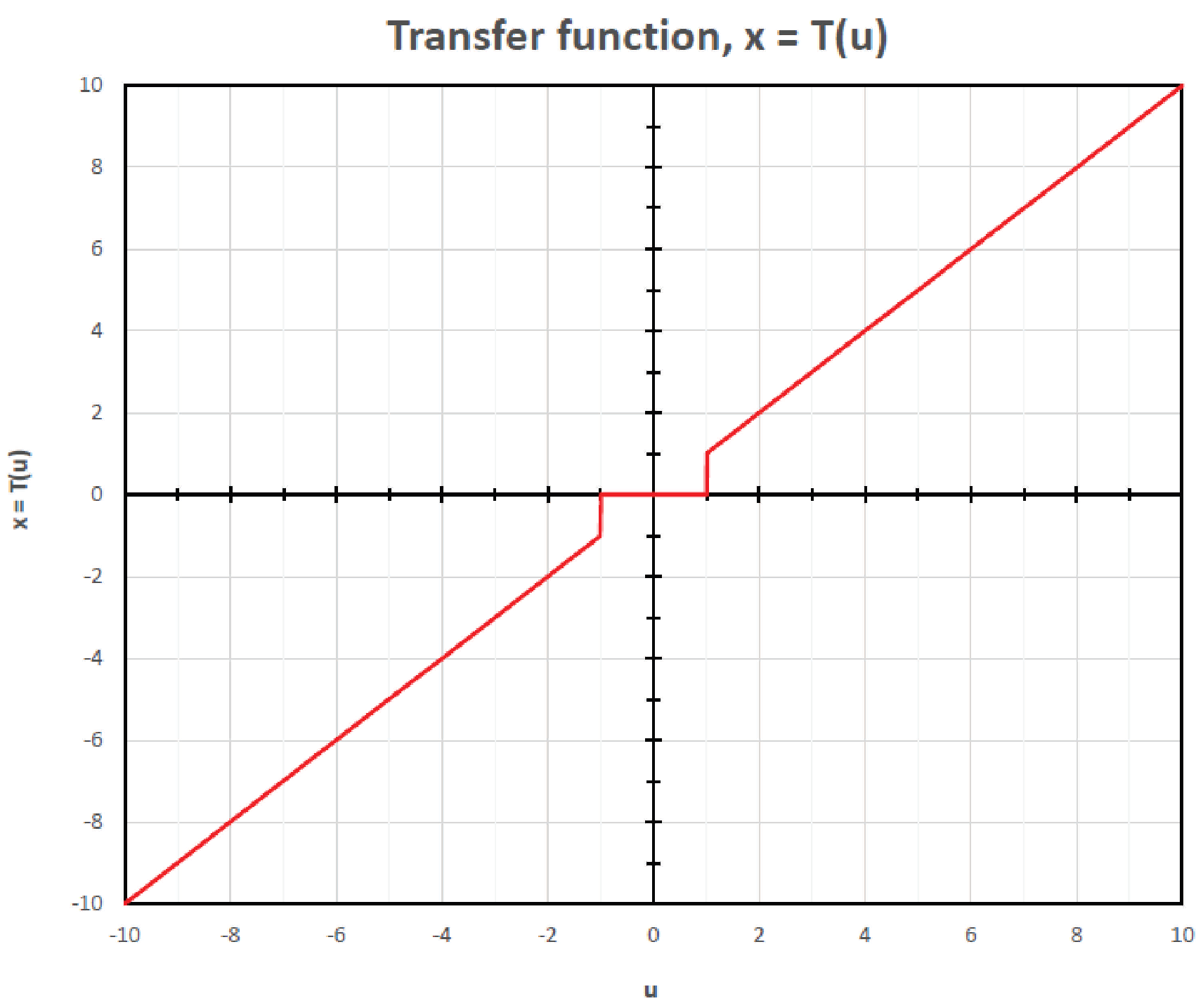
In Figure 3, we show the transfer function of our threshold function for V r e f = 1 . The transfer function is obtained from a circuit simulator. In the simulator, the open loop gain of OP-AMP1 is set to 10 8 and the open loop gain of OP-AMP2-to-OP-AMP4 is set to 10 5 . For the two MOSFETs, they are n-type with the following parameters: channel width = 100 μ m, channel length = 200 nm, transconductance = 118 μ A/V 2 , zero-bias threshold voltage = 430 mV and channel-length modulation = 60 mV 1 . From the figure, the transfer function quite matches our theoretical model with a large value of γ .

4.2. Circuit Structure

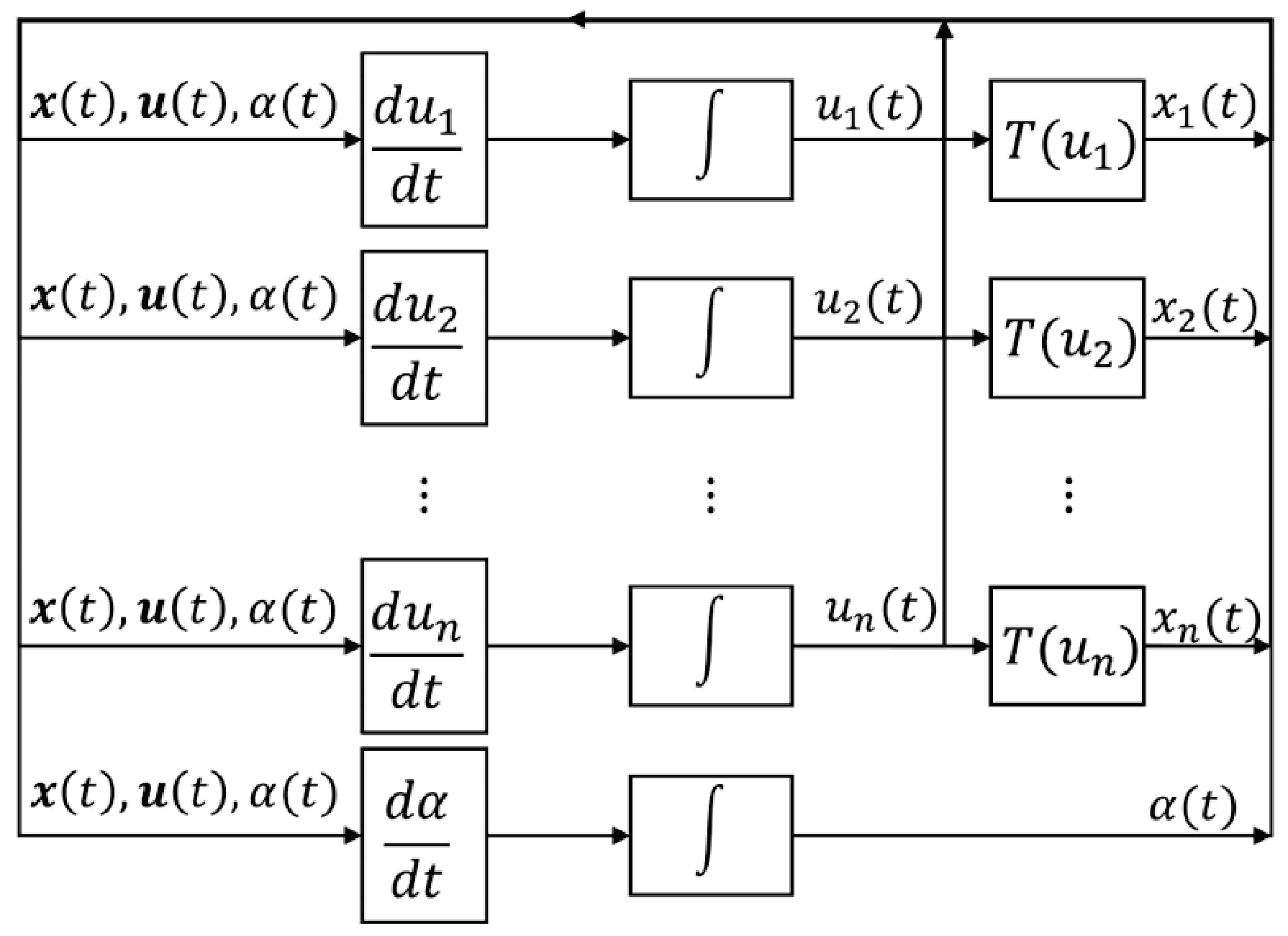
Figure 4 shows the analog realization of (21) in the block diagram level. In the realization, there are n blocks to compute d u i d t ’s. Inside each block, there are adders, multipliers, and square circuits. Additionally, there is a block to compute d α d t . The time derivatives d u i d t ’s and d α d t are then fed to the integrators to obtain internal variables u i ( t ) and α . In order to obtain the decision variables x i ( t ) ’s, the internal variables are fed to n thresholding elements (Figure 2), where V r e f = 1 / 2 .

4.3. Circuit Simulation

In this subsection, we use a small scale problem to verify our approach based on the Matlab Simulink platform. The problem details are:
  • n = 8 and m = 6 .
  • Measurement matrix:
    Φ = 1 8 1 1 1 1 1 1 1 1 1 1 1 1 1 1 1 1 1 1 1 1 1 1 1 1 1 1 1 1 1 1 1 1 1 1 1 1 1 1 1 1 1 1 1 1 1 1 1 1 .
  • Real sparse vector x = [ 2 , 0 , 0 , 0 , 0 , 0 , 2 , 0 ] T and noisy observation vector
    b = [ 0.0001 , 0.0038 , 1.4149 , 1.4145 , 1.4140 , 0.0035 ] T .
  • Noise tolerant parameter θ = 0.001 .
We build the Simulink file for our model, shown in Figure 4. We implement the thresholding function based on Figure 2. Other blocks are based on Simulink’s functional blocks. To verify our Simulink result, we also consider the discrete time simulation on (21). For digitization of (21), the discrete time simulation equations are
u ( t + Δ t ) = u ( t ) + Δ t d u d t
α ( t + Δ t ) = α ( t ) + Δ t d α d t .
where Δ t = 0.001 . Figure 5 shows the dynamics from the Simulink results and discrete time simulation. From the figure, the dynamics from the two approaches are nearly the same. The final outputs x are
Simulink : x = [ 1.9970 , 0 , 0 , 0 , 0 , 0 , 2.0037 , 0 ]
Discrete time : x = [ 1.9965 , 0 , 0 , 0 , 0 , 0 , 2.0032 , 0 ] .
Clearly, from Figure 5 and (23), both approaches produce the similar results.

5. Properties of the Dynamics

The first issue that we need to address is that equilibrium points of the LPNN-LPQC model should fulfill the KKT conditions of the LPQC problem, stated in (13). Otherwise, the LPNN-LPQC model cannot find out local/global minimums of the LPQC problem. Note that since the LPQC problem or the original 0 -norm CBPDN problem, stated in (2), are non-convex, few algorithms can ensure that their solutions are the global minimum.
The relationship between the equilibrium points of the LPNN-LPQC model and the KKT conditions are summarized in the following theorem.
Theorem 2. 
Given that { u * , α * } with α * 0 is an equilibrium point of the LPNN-LPQC model, this point corresponds to the KKT conditions of the LPQC problem. Note that x * = T ( u * ) .
Proof. 
From (21), when { u * , α * } is an equilibrium point, we
u * + x * + 2 α * 2 Φ T ( b Φ x * ) = 0 ,
2 α * ( b Φ x * 2 2 m θ 2 ) = 0 .
Clearly, (24a) is the same as (19a) with α * 2 = λ * . Additionally, when α * 0 , from (24b) becomes b Φ x * 2 2 m θ 2 = 0 which is the same (19b). The proof is completed. □
Theorem 2 tells us that equilibrium points of the LPNN-LPQC model corresponds to the KKT condition of the LPQC problem. Another concern is the stability of the equilibrium points of the LPNN-LPQC model. Theorem 3 presents the stability of the equilibrium points of the LPNN-LPQC model.
Theorem 3. 
Given a positive ϵ and for a sufficient large positive γ, if ( u * , α * ) with α 0 is an equilibrium point of the LPNN-LPQC model and for all i either | u i * | > 1 2 + 1 γ log γ ϵ or | u i * | < 1 2 1 γ log γ ϵ , then the equilibrium point is an asymptotically stable point.
Proof. 
The condition of either | u i | > 1 2 + 1 γ log γ ϵ or | u i | < 1 2 1 γ log γ ϵ is equivalent to for all i, | u i | [ 1 2 ζ , 1 2 + ζ ] , where ζ = 1 γ log γ ϵ . With the condition, we define two index sets, Γ u and Γ u c , given by
  • active set Γ u : If | u i | > 1 + ζ , then i Γ u .
  • inactive set Γ u c : If | u i | < 1 ζ , then i Γ u c .
Obviously, for a given ϵ and a sufficient large γ , ζ tends to zero and the value of ζ can be arbitrary small. Thus, the inactive neurons have nearly no effect on the dynamics, i.e., T ( u i ) tends to 0 for sufficient large γ (see Property 3).
For a given a , we define a Γ u as the vector composed of the elements of a indexed by Γ u and a Γ u c as the vector composed of the elements of a indexed by Γ u c . Similarly, given a matrix Φ , we define Φ Γ u as the matrix composed of the columns of Φ indexed by Γ u and Φ Γ u c as the matrix composed of the columns of Φ indexed by Γ u c .
Now, we consider the dynamics near u * and α * . We have two index sets Γ u * and Γ u * c As mentioned in the above, for inactive states x Γ u * c 0 for sufficient large γ . The dynamics given in (21) can be rewritten as:
d u Γ u * d t = u Γ u * + x Γ u * + 2 α 2 Φ Γ u * ( b Φ Γ u * x Γ u * ) ,
d α d t = 2 α ( b Φ Γ u * x Γ u * 2 2 m θ 2 ) ,
d u Γ u * c d t = u Γ u * c + 2 α 2 Φ Γ u * c b Φ Γ u * x Γ u * .
Furthermore, the linearization of (25) around the equilibrium point ( u * , α * ) is
d u Γ u * d t d α d t d u Γ u * c d t = H u Γ u * u Γ u * c * α α * u Γ u * c u Γ u * c * ,
where “ H ” is the Jacobian matrix at ( u * , α * ) and it is given by
H = [ d u ˙ Γ u * d u Γ u * d u ˙ Γ u * d α d u ˙ Γ u * d u Γ u * c d α ˙ d u Γ u * d α ˙ d α d α ˙ d u Γ u * c d u ˙ Γ u * c d u Γ u * d u ˙ Γ u * c d α d u ˙ Γ u * c d u Γ u * c ] ( u , α ) = ( u * , α * ) .
From the given condition, for active nodes, we have d x i / d u i 1 , and for inactive nodes d x i / d u i 0 . After deriving the sub-matrices in (27), we obtain
H = [ 2 α ¯ 2 Φ Γ ¯ Φ Γ ¯ 4 α ¯ Φ Γ ¯ ( b Φ Γ ¯ x ¯ Γ ¯ ) 4 α ¯ ( b Φ Γ ¯ x ¯ Γ ¯ ) Φ Γ ¯ 0 2 α ¯ 2 Φ Γ c ¯ Φ Γ ¯ 4 α ¯ Φ Γ c ¯ ( b Φ Γ ¯ x ¯ Γ ¯ ) I ] ,
where ∅ denotes a matrix of zero with appropriate size. Following the proof logic of Theorem 5 in [8], one can find that all eigenvalues of H are with positive real part. Therefore, according to the classical control theory, the corresponding equilibrium point ( u * , α * ) is asymptotically stable. The proof is completed. □

6. Experiment Results

6.1. Comparison Algorithms and Settings

This section compares our proposed LPNN-LPQC model with a number of digital numerical methods and analog neural methods. The comparison numerical methods are SPGL1 [30,50], MCP [35], AMP [37], 0 -ADMM [39,40], 0 -ZAP [38], NIHT [36], and ECME [41]. The comparison analog methods are IPNNSR [11] and PNN- 1 [13].
The seven numerical algorithms are described as follows. The SPGL1 [30,50] is a standard 1 -norm approach. The MCP [35] is based on the approximation of the 0 -norm function and its turning parameters are selected by cross validation. The NIHT [36], ECME [41], and AMP [37] are iterative algorithms, and they handle the 0 -norm term by the hard thresholding concept. The 0 -ADMM [39,40] uses the frameworks of ADMM and hard thresholding. The 0 ZAP [38] utilizes the idea of adaptive filter and projection. The two analog comparison models are IPNNSR [11] and PNN- 1 [13], and are developed based the projection concepts.
The setting of our experiment follows that of the experiment in [51]. The measurement matrix Φ is a random ± 1 / m matrix. The dimension n of the sparse signal x is 4096. A sparse signal contains k non-zero elements which locations are randomly chosen with uniform distribution. Their corresponding value are random ± 1 . In our experiment we set k = { 75 , 100 , 125 } .

6.2. Parameter Settings

To conduct the experiment, we need to select some parameters for the proposed method and comparison methods. In our proposed analog method, there are two tuning parameters which are γ and κ . To make the approximation p -norm close to the 0 norm, we should use a large γ . In our experiment, we set γ = 10 , 000 . Parameter κ is used to control the minimum value of the magnitudes of the decision variables x i . In our experiment, we set κ = 1 2 and Δ t = 0.0001 .
The SPGL1 package is used to solve
min x b Φ x 2 2 subject to x 1 k ,
where k is the number of non-zero elements in x . In the experiment, we set the maximum number of iterations to 100,000.
The MCP algorithm is used to solve
min x b Φ x 2 2 + P ( λ , γ ) ( x ) ,
where P ( λ , γ ) ( x ) is a penalty function to control the sparsity of the solution, and λ and γ are parameters in P ( λ , γ ) ( x ) . We set γ = 1.5 and use a linear search to obtain the best value of λ . We set the maximum number of iterations to 100,000.
The AMP, NIHT, and ECME algorithms are used to solve
min x b Φ x 2 2 subject to x 0 k ,
where k is the number of non-zero elements in x . We set the maximum number of iterations to 100,000.
The 0 -ADMM algorithm is used to solve
min x b Φ x 2 2 subject to x 0 k ,
where k is the number of non-zero elements in x . In 0 -ADMM, there is an augmented Lagrangian parameter ρ . It is set to 0.5 . The maximum number of iterations to 100,000.
The 0 -ZAP algorithm is used to solve
min x b Φ x 2 2 + γ x 0 ,
where γ is used to control the sparsity of the solution vector. We use a linear search to obtain the best value of γ . In addition, there are two parameter κ and α . In the experiment, κ = 0.001 and α = 2 . Additionally, the maximum number of iterations is 100,000.
The IPNNSR and PNN- 1 analog models are used to solve
min x x 1 subject to b = Φ x .
For IPNNSR, we set Δ t = 1 . For PNN- 1 , we set Δ t = 0.01 .

6.3. Convergence

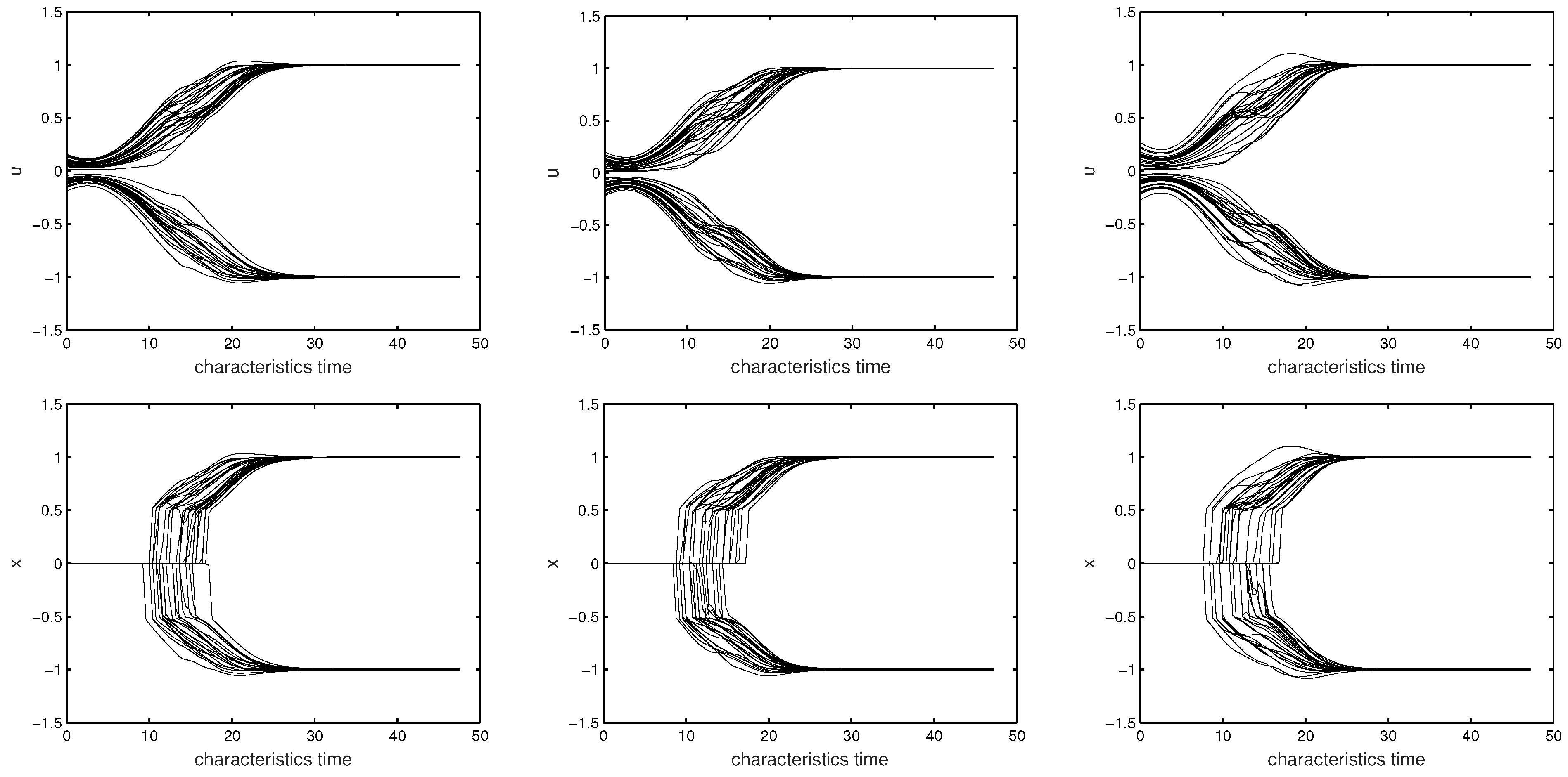
The proposed algorithm is an analog neural network. Hence, one important issue is the time to reach the equilibrium. Here, we conduct an experiment to empirically study the convergent time. Some typical dynamics are given in Figure 6. In the figure, the first row is the case of k = 75 and m = 500 , the second row is the case of k = 100 and m = 600 , and the third row is the case of k = 125 and m = 700 . Since there are 4096 elements in the decision variable vector x , the legibility of the figure will be very poor, if we plot all u i ( t ) ’s and x i ( t ) ’s in the figure. Therefore, we only plot the dynamics of the u i ( t ) ’s and x i ( t ) ’s whose original x i values are non-zero. From the figure, it can be seen that within 20–40 characteristic time units, the dynamics of our proposed analog neural network settle down.

6.4. Comparison with Other Algorithms

To further analyze the performance of our proposed method, we compare it with seven numerical algorithms and two analog models.
The observation vectors are generated by the following noisy model:
b = Φ x + e
where e is a zero mean Gaussian noise with standard deviation σ = { 0.001 , 0.005 , 0.01 } . The experiments repeat 100 times with different measurement matrix, initial states, and sparse signals. For each instance we declare that it is successful if
x 0 x ^ 2 x 0 2 tol ,
where x 0 denotes the true signal, x ^ is the recovered signal, and tol is the tolerant value. In our experiment, we set t o l = 0.01 .
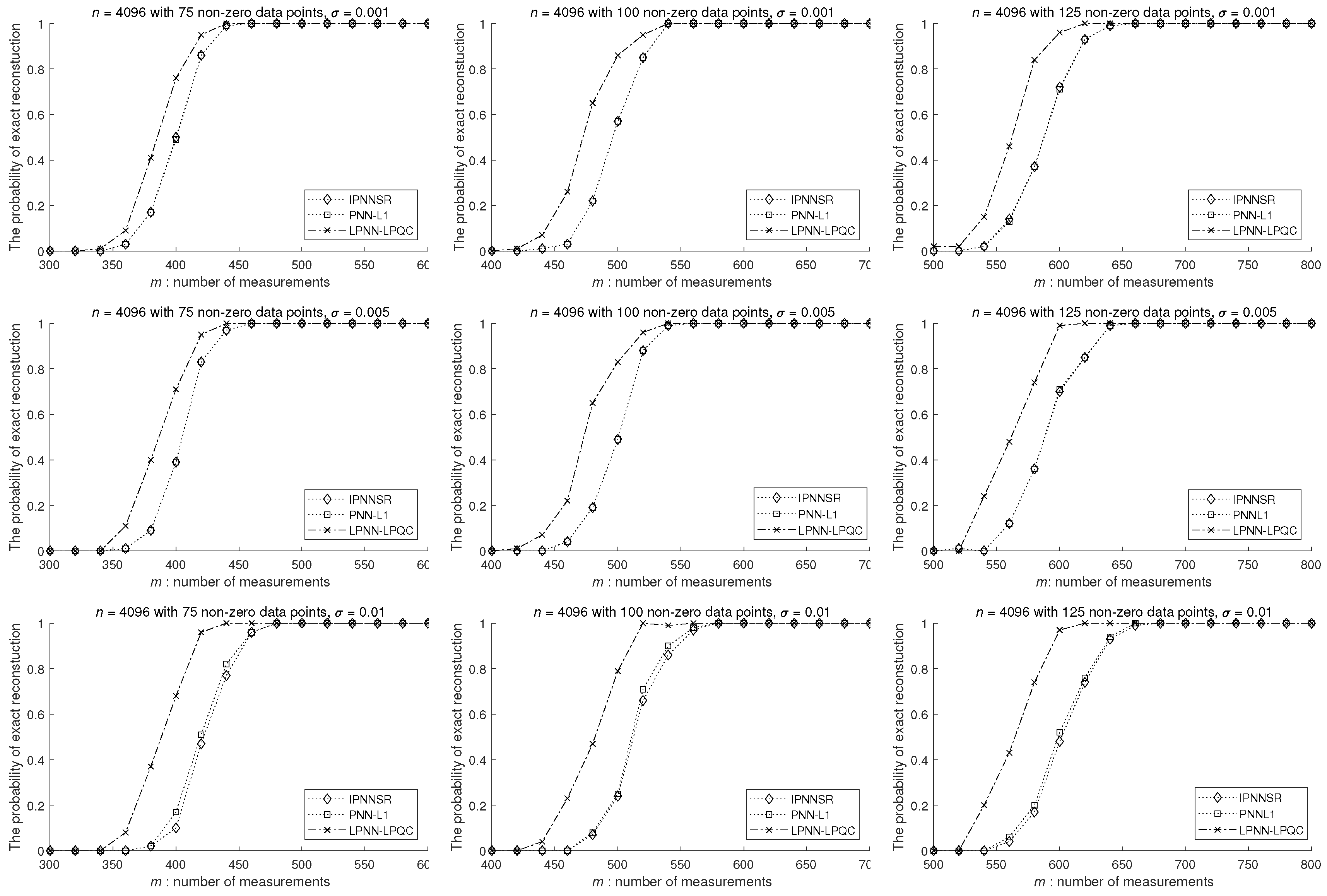
The successful rate results are shown in Figure 7. For all the algorithms, their performances are improved with the increasing numbers of measurements. From the figure, all 0 -norm and p -norm models are superior to the 1 models, including SPGL1, IPNNSR, and PNN- 1 . In addition, comparing with the seven numerical methods, our proposed method usually needs less measurements to obtain the same probability of exact reconstruction.
Comparing with the two analog models, IPNNSR and PNN- 1 , our LPNN-LPQC model is better. For example, with 125 non-zero elements and noise level equal to 0.01, the IPNNSR and PNN- 1 need around 650 measurement vectors, while our LPNN-LPQC needs around 575 to 600 measurement vectors only. The rationale of the improvement is that our model uses a 0 -norm approach, while IPNNSR and PNN- 1 are based on the 0 -norm.

6.5. Comparison with Other Analog Models

As the paper proposed an analog model, namely LPNN-LPQC, for sparse recovery, this subsection performs a deep discussion on the comparison among our proposed LPNN-LPQC, IPNNSR [11], and PNN- 1 [13]. We discuss three different aspects: probability of exact reconstruction and reconstruction error. In IPNNSR [11] and PNN- 1 [13], the circuit realization of thresholding operator and the projection operator were not addressed.

6.5.1. Successful Rate of Recall

Since Figure 7 shows the successful rates of all algorithms, it may not be easy to see the difference among the three analog models. In Figure 8, we only present the results of three analog models. From the figure, it can be seen that the performance of our LPNN-LPQC is better than that of IPNNSR and PNN- 1 . In particular, the performance improvement is significant when the number of non-zero elements is large and the noise level is high. For instance, with 125 non-zero elements and noise level = 0.01, the IPNNSR and PNN- 1 need around 650 measurements for high successful rates of recall, while our LPNN-LPQC needs around 575 to 600 measurements only.

6.5.2. MSE of Recall

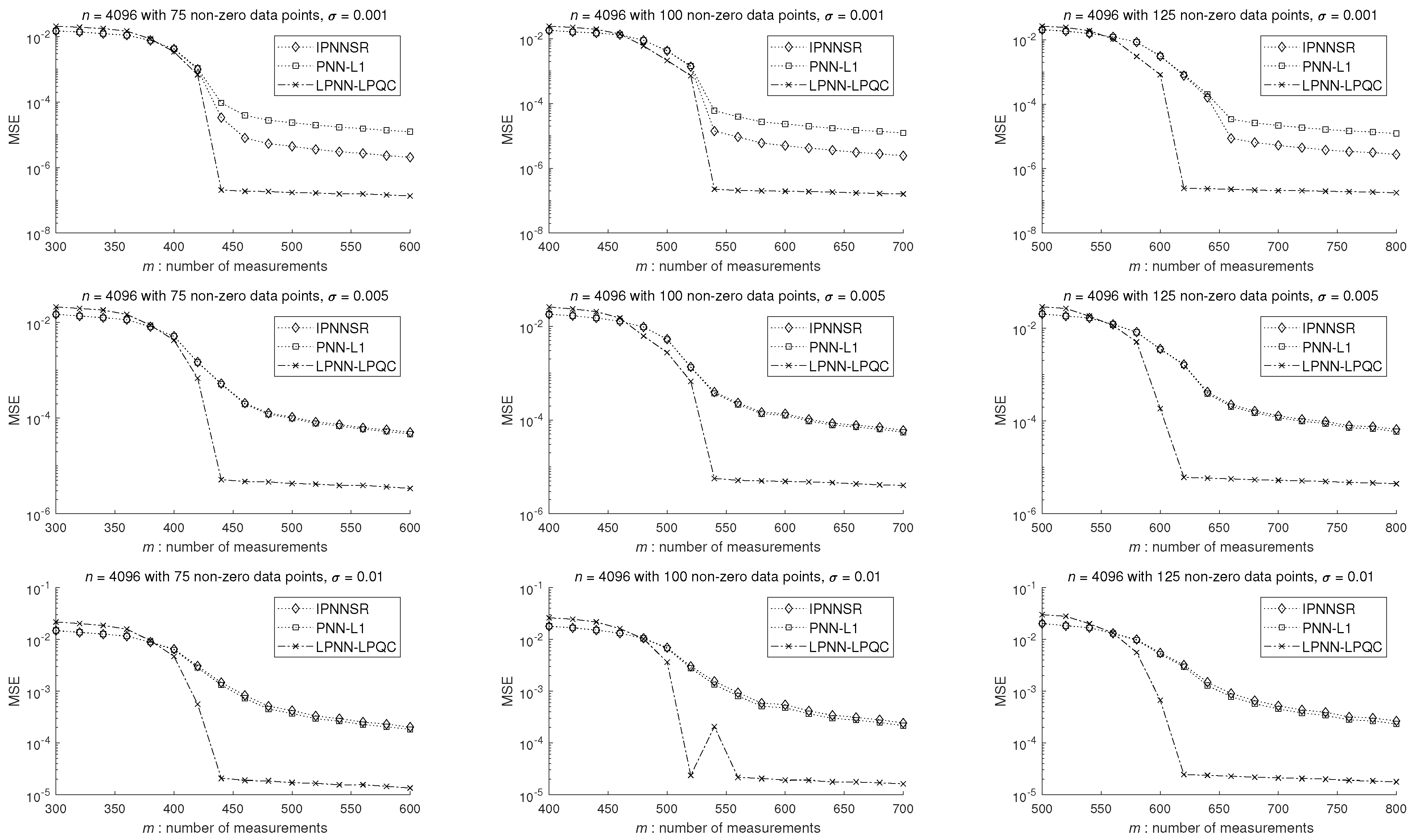
The successful rate results concern about whether the estimated x has the correct non-zero positions. Here, in Figure 9, we present the MSE versus the number of measurements used. From Figure 9, it can be seen that in terms of MSE, the performance of our LPNN-LPQC is much better than that of IPNNSR and PNN- 1 . In most cases, the MSE values of our proposed model are less than those of IPNNSR and PNN- 1 in one or two orders of magnitude. For example, for k = 75 , σ = 0.005 , and M = 450 , the MSE values of the IPNNSR and PNN- 1 are around 10 3 , while the MSE value of the proposed model is around 10 5 only.

7. Conclusions

This paper proposed a LPNN-LPQC method for sparse recovery under noise environment. The proposed algorithm is an analog neural network. We showed that the equilibrium points of the model satisfy the KKT conditions of the LPQC problem, and that the equilibrium points of the model are asymptotically stable. From the simulation results, we can see that the performance of the proposed algorithm is comparable to, even superior to many state-of-art 0 -norm or p -norm numerical methods. In addition, our proposed algorithm is superior to two analog models. We also presented the circuit realization for the thresholding element and performed circuit simulation for verifying our realization based on the MATLAB Simulink.
In our analysis, we assume that the realization of analog circuit does not have any time delay or synchronization problem. In fact, time delay and mis-synchronization may affect the stability of analog circuits [52,53]. Hence, one of future works is to investigate the behaviour of the proposed analog model with time delay or mis-synchronization.

Author Contributions

Conceptualization, H.W., R.F., C.-S.L. and A.G.C.; methodology, C.-S.L., H.W., R.F. and H.P.C.; software, H.W., R.F., H.P.C.; writing—original draft preparation, H.W.; writing—review and editing, C.-S.L.; supervision, C.-S.L. All authors have read and agreed to the published version of the manuscript.

Funding

This work was supported by the National Natural Science Foundation of China (Grant No. 62206178) and a research grant from City University of Hong Kong. Grant number 9678295.

Informed Consent Statement

Not applicable.

Data Availability Statement

Not applicable.

Conflicts of Interest

The authors declare no conflict of interest.

Abbreviations

The following abbreviations are used in this manuscript:
LPNNLagrange Programming Neural Network
LPNN-LPQCLPNN with p objective and Quadratic Constraint
CBPDNConstrained Basis Pursuit Denoise (CBPDN)
LCALocally Competitive Algorithm
KKTKarush Kuhn Tucker
MCPMinimax Concave Penalty
NIHTNormalized Iterative Hard Threshold
AMPApproximate Message Passing
0 - Z A P 0 -norm Zero Attraction Projection
0 - A D M M 0 -norm Alternating Direction Method of Multipliers
ECMEExpectation Conditional Maximization Either

Appendix A. Proof of Property 3

  • P3.a
Recall that f ( u ) = 1 1 + exp ( γ ( | u | 1 2 ) ) , and that f ( u ) is an even function. Clearly, T ( u ) = u f ( u ) is an odd function. First, since f ( u ) is an even function, the proof only presents the case of u 1 2 + 1 γ log 1 ϵ .
In the case of u 1 2 + 1 γ log 1 ϵ , f ( u ) is monotonic increasing. Hence
f ( u ) f ( 1 2 + 1 γ log 1 ϵ ) = 1 1 + exp ( log 1 ϵ ) = 1 1 + ϵ .
In addition, it is easy to show that f ( u ) is monotonic increasing, and that lim | u | f ( u ) = 1 . In conclusion, we have 1 1 + ϵ f ( u ) < 1 . P3.a is proved.
  • P3.b
Since f ( u ) is an even function, the proof only presents that the case of u 1 2 1 γ log 1 ϵ .
In the case of u 1 2 1 γ log 1 ϵ , f ( u ) is monotonic increasing. Hence, we have
f ( u ) f ( 1 2 1 γ log 1 ϵ ) = 1 1 + exp ( log 1 ϵ ) = ϵ 1 + ϵ .
Additionally, it is obvious that f ( u ) > 0 . Therefore, 0 < f ( u ) ϵ 1 + ϵ . P3.b is proved.
  • P3.c
For simplicity, let g ( u ) = exp ( γ ( | u | 1 2 ) ) . Thus, the derivative of T ( u ) can be rewritten as
d T ( u ) d u = 1 1 + g ( u ) + γ | u | g ( u ) ( 1 + g ( u ) ) 2
and the second derivative of T ( u ) is
d 2 T ( u ) d u 2 = 2 γ sign ( u ) g ( u ) ( 1 + g ( u ) ) 2 γ 2 u g ( u ) ( 1 + g ( u ) ) 2 + 2 γ 2 u g ( u ) 2 ( 1 + g ( u ) ) 3 .
Since T ( u ) is an odd function and d T ( u ) d u is an even function, we only present the proof for the case of u > 1 2 + 1 γ log γ ϵ . The proof consists of two parts. First, we show the monotonic property of d T ( u ) d u for u > 1 2 + 1 γ log γ ϵ . Second, the upper and lower bounds of d T ( u ) d u are established.
For the case of u > 1 2 + 1 γ log γ ϵ , we have 0 < g ( u ) < ϵ γ . The second derivative of T ( u ) in (A4) can be rewritten as:
d 2 T ( u ) d u 2 = g ( u ) · ( 2 γ γ 2 u ) ( 1 + g ( u ) ) + 2 γ 2 u g ( u ) ( 1 + g ( u ) ) 3 .
Since 0 < g ( u ) < ϵ / γ , we can deduce that
( 2 γ γ 2 u ) ( 1 + g ( u ) ) + 2 γ 2 u g ( u ) = 2 γ γ 2 u + ( 2 γ + γ 2 u ) g ( u ) < 2 γ γ 2 u + ( 2 γ + γ 2 u ) ϵ γ = 2 γ γ 2 u + 2 ϵ + 2 γ u ϵ < ( 2 γ + 4 ϵ ) γ u < 0 .
From (A5), (A6), g ( u ) > 0 , and ( 1 + g ( u ) ) 3 > 0 , we deduce that, if u > 1 2 + 1 γ log γ ϵ , then d 2 T ( u ) / d u 2 < 0 and d T ( u ) d u is monotonic decreasing. Thus, for u > 1 2 + 1 γ log γ ϵ , a lower bound on d T ( u ) d u is d T ( u ) d u | u . Since lim u g ( u ) = 0 and d T ( u ) d u | u = 1 , we have
d T ( u ) d u > 1 .
On the contrary, an upper bound in u > 1 2 + 1 γ log γ ϵ , is d T ( u ) d u | u = 1 2 + 1 γ log γ ϵ . The value of d T ( u ) d u | u = 1 2 + 1 γ log γ ϵ is
d T ( u ) d u | u = 1 2 + 1 γ log γ ϵ = 1 1 + ϵ γ + γ u ϵ γ ( 1 + ϵ γ ) 2 = γ 2 + γ ϵ + u ϵ γ 2 ( γ + ϵ ) 2 = ( γ + ϵ ) 2 + u ϵ γ 2 ϵ γ ϵ 2 ( γ + ϵ ) 2 = 1 + 1 2 γ 2 + γ log γ ϵ ϵ γ ( γ + ϵ ) 2 ϵ = 1 + 1 2 ( γ + ϵ ) 2 + ( log γ ϵ 1 ϵ ) γ ϵ 1 2 ϵ 2 ( γ + ϵ ) 2 ϵ < 1 + ϵ 2 + ( log γ ϵ 1 ϵ ) γ ( γ + ϵ ) 2 ϵ < 1 + 3 ϵ 2 .
From (A5) and (A6), and the fact that d T ( u ) d u is an even function, we can conclude that for a sufficiently large γ , if | u | > 1 2 + 1 γ log γ ϵ , then 1 < d T ( u ) d u < 1 + 3 2 ϵ . The proof of P3.c is completed.
  • P3.d
The proof consists of two parts. First, we show the monotonic properties of d T ( u ) d u for | u | < 1 2 1 γ log γ ϵ . Second, the upper and lower bounds of d T ( u ) d u are established. Since T ( u ) is an odd function and d T ( u ) d u is an even function, we only need to consider the region of u < 1 2 1 γ log γ ϵ .
For 0 < u < 1 2 1 γ log γ ϵ , sign ( u ) > 0 , g ( u ) is monotonic decreasing, and exp ( γ ) > g ( u ) > γ ϵ . In this region, the second derivative of T ( u ) is
d 2 T ( u ) d u 2 = 2 γ g ( u ) ( 1 + g ( u ) ) 2 γ 2 u g ( u ) ( 1 + g ( u ) ) 2 + 2 γ 2 u g ( u ) 2 ( 1 + g ( u ) ) 3 > γ 2 g ( u ) u ( 1 + g ( u ) ) 2 + 2 γ 2 u g ( u ) 2 ( 1 + g ( u ) ) 3 = ( g ( u ) 1 ) · γ 2 g ( u ) u ( 1 + g ( u ) ) 3 .
Obviously, in this region, γ 2 g ( u ) u ( 1 + g ( u ) ) 3 > 0 , and
g ( u ) 1 > γ ϵ 1 > 0 .
Hence, we can conclude that, for 0 < u < 1 2 1 γ log γ ϵ , d 2 T ( u ) / d u 2 > 0 and then d T ( u ) d u is monotonically increasing. For u < 1 2 1 γ log γ ϵ , the upper bound of d T ( u ) / d u exists when u = 1 2 1 γ log γ ϵ . The upper bound is
d T ( u ) d u | u = 1 2 1 γ log γ ϵ = 1 1 + γ ϵ + γ 2 | u | ϵ ( 1 + γ ϵ ) 2 = γ 2 | u | + ϵ + γ ( γ + ϵ ) 2 ϵ < 1 2 γ 2 + ϵ + γ ( γ + ϵ ) 2 ϵ = 1 2 ϵ + γ + ϵ + 2 γ ϵ 1 2 ϵ 2 ( γ + ϵ ) 2 ϵ < 3 2 ϵ .
In addition, a lower bound on d T ( u ) d u exists at u = 0 ,
d T ( u ) d u | u = 0 = 1 1 + exp ( γ ) > 0
To sum up, for a sufficiently large γ , if u < 1 2 1 γ log γ ϵ , then 0 < d T ( u ) d u < 3 2 ϵ . The proof of P3.d is completed.

Appendix B. Proof of Property 4

The continuity and differentiability of S ( x ) can be proved according to the following lemma [54].
Lemma A1. 
(Inverse function) Let ϕ be a strictly monotone continuous function on [ a , b ] , with ϕ differentiable at x 0 ( a , b ) and d ϕ d x | x = x 0 0 . Then ϕ 1 exists and is continuous and strictly monotone. Moreover, ϕ 1 is differentiable at y 0 = ϕ ( x 0 ) and
d ϕ 1 ( y ) d y | y = y 0 = 1 d ϕ d x | x = x 0 .
From (A3), one can easily verify that d T ( u ) d u > 0 , and that T ( u ) is a strictly monotone increasing continuous function. Based on Lemma A1, T 1 ( x ) exists. Additionally, it is continuous and differentiable at every point. Hence 1 2 S ( x ) = T 1 ( x ) x is a continuous and differentiable function. The proof is completed.

Appendix C. Proof of Property 5

  • Boundness: Now, we use the Taylor series of S ( x ) to estimate the values of S ( ± 1 2 ) . Since S ( x ) is an even function, the proof only presents the case of u > 1 2 + 1 γ log 1 ϵ .
First, we can use x = 1 4 to obtain the Taylor series expansion of 1 2 S ( x ) :
1 2 S ( x ) 1 2 S ( 1 4 ) + 1 2 S ( 1 4 ) ( x 1 4 ) + 1 2 1 2 S ( 1 4 ) ( x 1 4 ) 2 ,
where S ( 1 4 ) and S ( 1 4 ) are the first and second order derivatives of S ( x ) at x = 1 4 , respectively. Since 1 2 S ( x ) = u x = T 1 ( x ) x and T ( 1 2 ) = 1 4 , we obtain
1 2 S ( 1 4 ) = 1 2 1 4 = 1 4 .
Additionally, 1 2 S ( 1 4 ) = d T 1 ( x ) d x | x = 1 / 4 1 . As T ( 1 2 ) = 1 4 , from Lemma 2,
d T 1 ( x ) d x | x = 1 / 4 = 1 d T ( u ) d u | u = 1 2 .
Additionally, from (A3),
d T ( u ) d u | u = 1 2 = 2 + γ 4 .
From (A14)–(A17), for a small ϵ and a sufficient large γ ,
1 2 S ( x ) 1 2 S ( 1 4 ) + 1 4 ( x 1 4 ) + 1 2 ( 4 2 + γ 1 ) ( x 1 4 ) 2 1 2 S ( 1 2 ) + 1 4 ( x 1 4 ) 1 2 ( x 1 4 ) 2 .
Thus, we have
1 2 S ( 1 2 ) 1 2 S ( 1 4 ) + 1 32 , and 1 2 S ( 0 ) 1 2 S ( 1 4 ) 3 32 .
As 1 2 S ( 0 ) = 0 , we obtain 1 2 S ( 1 2 ) 1 8 . Similarly, it is also easy to obtain that 1 2 S ( 1 2 ) 1 8 .
Now we would like to know for u > 1 2 + 1 γ log 1 ϵ , i.e., x > T ( 1 2 + 1 γ log 1 ϵ ) , what the value of 1 2 S ( x ) is.
Let u 0 = 1 2 + 1 γ log 1 ϵ and x 0 = T ( u 0 ) . Since S ( x ) is an even function and is monotonic increasing (for x > 0 ), for x x 0 , we have
1 2 S ( x ) 1 2 S ( x 0 ) = x 0 x ( u χ ) d χ .
From P3, we have u ( 1 + ϵ ) x . Thus,
1 2 S ( x ) 1 2 S ( x 0 ) x 0 x ϵ χ d χ .
Thus, for a sufficient small ϵ , 1 2 S ( x ) 1 2 S ( x 0 ) 0 . In addition, for sufficient small ϵ and sufficient large γ , u 0 1 2 . As 1 2 S ( 1 2 ) 1 8 , we have 1 2 S ( x ) 1 8 for u 1 2 + 1 γ log 1 ϵ .
Sparsity: Since 1 2 S ( x ) is an even function, we only show the proof for 0 < x < T ( 1 2 1 γ log 1 ϵ ) , i.e., the case of 0 < u < 1 2 1 γ log 1 ϵ . Let u 0 = 1 2 1 γ log 1 ϵ and x 0 = T ( u 0 ) . For x > 0 , 1 2 S ( x ) is a monotonical increasing. Hence, we have 0 = 1 2 S ( 0 ) < 1 2 S ( x ) < 1 2 S ( x 0 ) . Therefore, we have
1 2 S ( x 0 ) 1 2 S ( 0 ) = 0 x 0 u χ d χ .
From P3.b, we can deduce that 0 < x 0 ϵ u 0 1 + ϵ . For a sufficient small ϵ , x 0 ϵ u 0 1 + ϵ 0 . Obviously, in this region u χ is bounded. Hence, we have 1 2 S ( x 0 ) 0 . As 0 = 1 2 S ( 0 ) < 1 2 S ( x ) < 1 2 S ( x 0 ) , we can say that 1 2 S ( x ) 0 for 0 x x 0 . In conclusion, 1 2 S ( x ) 0 if | x | < T ( 1 2 1 η log 1 ϵ ) . The proof is completed.

References

  1. Chua, L.; Lin, G.N. Nonlinear programming without computation. IEEE Trans. Circuits Syst. 1984, 31, 182–188. [Google Scholar] [CrossRef]
  2. Tank, D.; Hopfield, J. Simple ‘neural’ optimization networks: An A/D converter, signal decision circuit, and a linear programming circuit. IEEE Trans. Circuits Syst. 1986, 33, 533–541. [Google Scholar] [CrossRef] [Green Version]
  3. Xia, Y.; Leung, H.; Wang, J. A projection neural network and its application to constrained optimization problems. IEEE Trans. Circuits Syst. Fundam. Theory Appl. 2002, 49, 447–458. [Google Scholar]
  4. Xia, Y.; Wang, J. A general projection neural network for solving monotone variational inequalities and related optimization problems. IEEE Trans. Neural Netw. 2004, 15, 318–328. [Google Scholar] [CrossRef] [PubMed]
  5. Wang, H.; Lee, C.M.; Feng, R.; Leung, C.S. An analog neural network approach for the least absolute shrinkage and selection operator problem. Neural Comput. Appl. 2018, 29, 389–400. [Google Scholar] [CrossRef]
  6. Wang, Y.; Li, X.; Wang, J. A neurodynamic optimization approach to supervised feature selection via fractional programming. Neural Netw. 2021, 136, 194–206. [Google Scholar] [CrossRef]
  7. Bouzerdoum, A.; Pattison, T.R. Neural network for quadratic optimization with bound constraints. IEEE Trans. Neural Netw. 1993, 4, 293–304. [Google Scholar] [CrossRef]
  8. Feng, R.; Leung, C.S.; Constantinides, A.G.; Zeng, W.J. Lagrange Programming Neural Network for Nondifferentiable Optimization Problems in Sparse Approximation. IEEE Trans. Neural Netw. Learn. Syst. 2017, 28, 2395–2407. [Google Scholar] [CrossRef]
  9. Wang, H.; Feng, R.; Leung, A.C.S.; Tsang, K.F. Lagrange programming neural network approaches for robust time-of-arrival localization. Cogn. Comput. 2018, 10, 23–34. [Google Scholar] [CrossRef]
  10. Shi, Z.; Wang, H.; Leung, C.S.; So, H.C.; Member EURASIP. Robust MIMO radar target localization based on Lagrange programming neural network. Signal Process. 2020, 174, 107574. [Google Scholar] [CrossRef]
  11. Liu, Q.; Wang, J. L_{1}-minimization algorithms for sparse signal reconstruction based on a projection neural network. IEEE Trans. Neural Netw. Learn. Syst. 2015, 27, 698–707. [Google Scholar] [CrossRef] [PubMed]
  12. Yan, Z.; Le, X.; Wen, S.; Lu, J. A Continuous-Time Recurrent Neural Network for Sparse Signal Reconstruction Via 1 Minimization. In Proceedings of the 2018 Eighth International Conference on Information Science and Technology (ICIST), Cordoba, Granada, and Seville, Spain, 30 June–6 July 2018; pp. 43–49. [Google Scholar] [CrossRef]
  13. Wen, H.; Wang, H.; He, X. A Neurodynamic Algorithm for Sparse Signal Reconstruction with Finite-Time Convergence. Circuits Syst. Signal Process. 2020, 39, 6058–6072. [Google Scholar] [CrossRef]
  14. Donoho, D.; Huo, X. Uncertainty principles and ideal atomic decomposition. IEEE Trans. Inf. Theory 1999, 47, 2845–2862. [Google Scholar] [CrossRef] [Green Version]
  15. Donoho, D.L.; Elad, M. Optimally sparse representation in general (nonorthogonal) dictionaries via l1 minimization. Proc. Natl. Acad. Sci. USA 2003, 100, 2197–2202. [Google Scholar] [CrossRef] [PubMed] [Green Version]
  16. Chartrand, R. Exact reconstruction of sparse signals via nonconvex minimization. IEEE Signal Process. Lett. 2007, 14, 707–710. [Google Scholar] [CrossRef]
  17. Blumensath, T.; Davies, M.E. Iterative thresholding for sparse approximations. J. Fourier Anal. Appl. 2008, 14, 629–654. [Google Scholar] [CrossRef] [Green Version]
  18. Jin, D.; Yang, G.; Li, Z.; Liu, H. Sparse recovery algorithm for compressed sensing using smoothed 0-norm and randomized coordinate descent. Mathematics 2019, 7, 834. [Google Scholar] [CrossRef] [Green Version]
  19. Stanković, L.; Sejdić, E.; Stanković, S.; Daković, M.; Orović, I. A tutorial on sparse signal reconstruction and its applications in signal processing. Circuits Syst. Signal Process. 2019, 38, 1206–1263. [Google Scholar] [CrossRef]
  20. Stanković, I.; Ioana, C.; Daković, M. On the reconstruction of nonsparse time-frequency signals with sparsity constraint from a reduced set of samples. Signal Process. 2018, 142, 480–484. [Google Scholar] [CrossRef]
  21. Dai, C.; Che, H.; Leung, M.F. A neurodynamic optimization approach for L1 minimization with application to compressed image reconstruction. Int. J. Artif. Intell. Tools 2021, 30, 2140007. [Google Scholar] [CrossRef]
  22. Bioucas-Dias, J.M.; Figueiredo, M.A. A new TwIST: Two-step iterative shrinkage/thresholding algorithms for image restoration. IEEE Trans. Image Process. 2007, 16, 2992–3004. [Google Scholar] [CrossRef] [PubMed] [Green Version]
  23. Kong, X.; Zhao, Y.; Xue, J.; Chan, J.C.W.; Kong, S.G. Global and local tensor sparse approximation models for hyperspectral image destriping. Remote Sens. 2020, 12, 704. [Google Scholar] [CrossRef] [Green Version]
  24. Costanzo, S.; Rocha, Á.; Migliore, M.D. Compressed sensing: Applications in radar and communications. Sci. World J. 2016, 2016, 5407415. [Google Scholar] [CrossRef] [PubMed] [Green Version]
  25. Li, S.; Zhao, G.; Zhang, W.; Qiu, Q.; Sun, H. ISAR imaging by two-dimensional convex optimization-based compressive sensing. IEEE Sens. J. 2016, 16, 7088–7093. [Google Scholar] [CrossRef]
  26. Craven, D.; McGinley, B.; Kilmartin, L.; Glavin, M.; Jones, E. Compressed sensing for bioelectric signals: A review. IEEE J. Biomed. Health Inform. 2014, 19, 529–540. [Google Scholar] [CrossRef]
  27. Chen, S.S.; Donoho, D.L.; Saunders, M.A. Atomic decomposition by basis pursuit. SIAM Rev. 2001, 43, 129–159. [Google Scholar] [CrossRef] [Green Version]
  28. Osborne, M.R.; Presnell, B.; Turlach, B.A. A new approach to variable selection in least squares problems. IMA J. Numer. Anal. 2000, 20, 389–403. [Google Scholar] [CrossRef] [Green Version]
  29. Candes, E.; Romberg, J. l1-Magic. 2017. Available online: https://candes.su.domains/software/l1magic/downloads/l1magic.pdf (accessed on 1 December 2022).
  30. van den Berg, E.; Friedlander, M.P. SPGL1: A Solver for Sparse Least Squares. 2007. Available online: https://friedlander.io/spgl1/ (accessed on 1 December 2022).
  31. Rozell, C.J.; Johnson, D.H.; Baraniuk, R.G.; Olshausen, B.A. Sparse coding via thresholding and local competition in neural circuits. Neural Comput. 2008, 20, 2526–2563. [Google Scholar] [CrossRef]
  32. Engan, K.; Rao, B.D.; Kreutz-Delgado, K. Regularized FOCUSS for subset selection in noise. In Proceedings of the NORSIG 2000, Kolmarden, Sweden, 13–15 June 2000; pp. 247–250. [Google Scholar]
  33. Rao, B.D.; Kreutz-Delgado, K. An affine scaling methodology for best basis selection. IEEE Trans. Signal Process. 1999, 47, 187–200. [Google Scholar] [CrossRef] [Green Version]
  34. Zhang, C.H. Nearly unbiased variable selection under minimax concave penalty. Ann. Stat. 2010, 38, 894–942. [Google Scholar] [CrossRef]
  35. Breheny, P.; Huang, J. Coordinate descent algorithms for nonconvex penalized regression, with applications to biological feature selection. Ann. Appl. Stat. 2011, 5, 232. [Google Scholar] [CrossRef] [PubMed] [Green Version]
  36. Blumensath, T.; Davies, M.E. Normalized iterative hard thresholding: Guaranteed stability and performance. IEEE J. Sel. Top. Signal Process. 2010, 4, 298–309. [Google Scholar] [CrossRef] [Green Version]
  37. Donoho, D.L.; Maleki, A.; Montanari, A. Message-passing algorithms for compressed sensing. Proc. Natl. Acad. Sci. USA 2009, 106, 18914–18919. [Google Scholar] [CrossRef] [PubMed] [Green Version]
  38. Jin, J.; Gu, Y.; Mei, S. A stochastic gradient approach on compressive sensing signal reconstruction based on adaptive filtering framework. IEEE J. Sel. Top. Signal Process. 2010, 4, 409–420. [Google Scholar] [CrossRef] [Green Version]
  39. Boyd, S.; Parikh, N.; Chu, E.; Peleato, B.; Eckstein, J. Distributed optimization and statistical learning via the alternating direction method of multipliers. Found. Trends Mach. Learn. 2011, 3, 1–122. [Google Scholar] [CrossRef]
  40. Song, C.; Xia, S.T. Alternating direction algorithms for ∖ell_0 regularization in compressed sensing. arXiv 2016, arXiv:1604.04424. [Google Scholar]
  41. Qiu, K.; Dogandzic, A. ECME thresholding methods for sparse signal reconstruction. arXiv 2010, arXiv:1004.4880. [Google Scholar]
  42. Zhang, S.; Constantinidies, A.G. Lagrange Programming Neural Networks. IEEE Trans. Circuits Syst. II 1992, 39, 441–452. [Google Scholar] [CrossRef]
  43. Shi, Z.; Wang, H.; Leung, C.S.; So, H.C.; Liang, J.; Tsang, K.F.; Constantinides, A.G. Robust ellipse fitting based on Lagrange programming neural network and locally competitive algorithm. Neurocomputing 2020, 399, 399–413. [Google Scholar] [CrossRef]
  44. Balavoine, A.; Rozell, C.; Romberg, J. Global convergence of the locally competitive algorithm. In Proceedings of the IEEE Signal Processing Education Workshop (DSP/SPE) 2011, Sedona, AZ, USA, 4–7 January 2011; pp. 431–436. [Google Scholar]
  45. Pandey, O. Operational Amplifier (Op-Amp). In Electronics Engineering; Springer: Berlin/Heidelberg, Germany, 2022; pp. 233–270. [Google Scholar]
  46. Bult, K.; Wallinga, H. A CMOS four-quadrant analog multiplier. IEEE J. Solid-State Circuits 1986, 21, 430–435. [Google Scholar] [CrossRef] [Green Version]
  47. Chen, C.; Li, Z. A low-power CMOS analog multiplier. IEEE Trans. Circuits Syst. II Express Briefs 2006, 53, 100–104. [Google Scholar] [CrossRef]
  48. Filanovsky, I.; Baltes, H. Simple CMOS analog square-rooting and squaring circuits. IEEE Trans. Circuits Syst. I Fundam. Theory Appl. 1992, 39, 312–315. [Google Scholar] [CrossRef]
  49. Sakul, C. A new CMOS squaring circuit using voltage/current input. In Proceedings of the 23rd International Technical Conference on Circuits/Systems, Computers and Communications ITC-CSCC, Phuket, Thailand, 5–8 July 2008; pp. 525–528. [Google Scholar]
  50. van den Berg, E.; Friedlander, M.P. Probing the Pareto frontier for basis pursuit solutions. SIAM J. Sci. Comput. 2008, 31, 890–912. [Google Scholar] [CrossRef] [Green Version]
  51. Ji, S.; Xue, Y.; Carin, L. Bayesian compressive sensing. IEEE Trans. Signal Process. 2008, 56, 2346–2356. [Google Scholar] [CrossRef]
  52. Vadivel, R.; Hammachukiattikul, P.; Zhu, Q.; Gunasekaran, N. Event-triggered synchronization for stochastic delayed neural networks: Passivity and passification case. Asian J. Control 2022. [Google Scholar] [CrossRef]
  53. Chanthorn, P.; Rajchakit, G.; Humphries, U.; Kaewmesri, P.; Sriraman, R.; Lim, C.P. A delay-dividing approach to robust stability of uncertain stochastic complex-valued hopfield delayed neural networks. Symmetry 2020, 12, 683. [Google Scholar] [CrossRef]
  54. Spruck, J. Strictly Monotone Functions and the Inverse Function Theorem. Lecture Notes in MATH–405. Available online: https://math.jhu.edu/~js/math405/405.monotone.pdf (accessed on 24 November 2021).
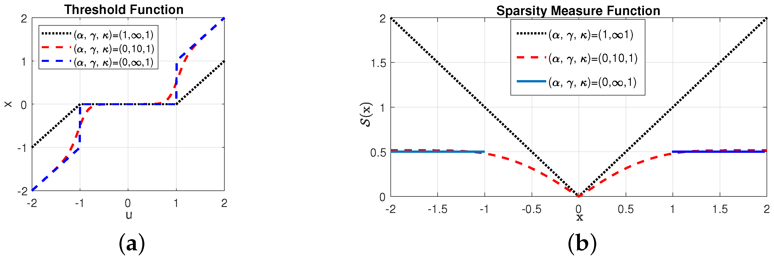
Figure 1. Threshold function and sparsity measure function. (a) The shape of T α , γ , κ ( u i ) under various settings. (b) Sparsity measure function. For α = 0 , γ and κ = 1 , the value of x cannot be in the range of ( 0 , 1 ) based on the property of the ideal thresholding function T 0 , , 1 ( u ) .
Mathematics 10 04801 g001
Figure 2. (a) Circuit for the thresholding function T ( x ) . (b) Equivalent circuit of the thresholding function T ( x ) when the magnitude of input is greater than V r e f . (c) Equivalent circuit of the thresholding function T ( x ) when the magnitude of input is less than or equal to V r e f .
Mathematics 10 04801 g002
Figure 3. Thresholding function T ( x ) obtained from the circuit simulation of Figure 2 with V r e f = 1 .
Mathematics 10 04801 g003
Figure 4. Analog realization of (21) in the block diagram level.
Mathematics 10 04801 g004
Figure 5. Dynamics obtained from Simulink and discrete time simulation.
Mathematics 10 04801 g005
Figure 6. Typical dynamics of u and x for the LPNN-LPQC model, where n = 4096 . The first column: k = 75 , m = 500 . The second column: k = 100 , m = 600 . The third column, k = 125 , m = 700 . In all sub-figures, we only show the dynamics of the u i ’s and x i ’s whose original x i values are non-zero, because there are 4096 curves in each sub-figure when we show all the dynamics for u i ’s and x i ’s.
Mathematics 10 04801 g006
Figure 7. Simulation results of different algorithms, where n = 4096 . For the first column, k = 75 . For the second column, k = 100 . For the third column, k = 125 . The three rows are based on three different noise levels. The experiments are repeated 100 times using different settings.
Mathematics 10 04801 g007
Figure 8. Comparison with other analog models on probability of reconstruction, where n = 4096 . For the first column, k = 75 . For the second column, k = 100 . For the third column, k = 125 . The three rows are based on three different noise levels. The experiments are repeated 100 times using different settings.
Mathematics 10 04801 g008
Figure 9. Comparison with other analog models on MSE, where n = 4096 . For the first column, k = 75 . For the second column, k = 100 . For the third column, k = 125 . The three rows are based on three different noise levels. The experiments are repeated 100 times using different settings.
Mathematics 10 04801 g009
Publisher’s Note: MDPI stays neutral with regard to jurisdictional claims in published maps and institutional affiliations.