Advanced Algorithms in Automatic Generation Control of Hydroelectric Power Plants

Abstract

The problem of load distribution between hydraulic units at hydropower plants is a difficult task due to the nonlinearity of hydro turbine characteristics and individual peculiarities of the generation units, in which operating conditions are often different. It is necessary to apply the most up-to-date optimization methods that take into account the nonlinearity of the turbine characteristics. The methods must also consider strict constraints on the operation conditions of the power equipment when searching for the extremum of the objective function specified in the form of equalities and inequalities. When solving the aforementioned optimization problem, the constraints on computing capacities of the digital automatic generation control systems that must operate in real-time mode were taken into account. To solve the optimization task, the interior point method was analyzed and the method of Lagrange multipliers was modified so that it could minimize turbine discharge and active energy losses in the windings of the power generators and unit power transformers. The article presents the simulation results of the developed optimization algorithms and the results of the field tests of the automatic generation control system executing the proposed algorithms. All of the tests showed a fairly high efficiency of the proposed optimization methods in real operation conditions.

1. Introduction

Hydroelectric power plants (HPPs) gained great importance today. Not only these types of power plants are environmentally friendly and generate cheap electrical energy, but also are powerful tools for controlling the state of the electric power systems. The share of the electric energy produced by solar and wind power plants known by their stochastic nature constantly grows and so does the need for the fast and qualitative control of the power systems having a significant share of renewable energy sources [1,2,3,4].

However, being a flexible source of electric power, HPPs do not always provide high-quality control of the power system parameters [5,6,7]. The solution could be the application of wide-area measurement systems (WAMS), which allows the detection of active power fluctuations in bulk power systems, resulting from incorrect operation of automatic generation controllers and speed governors [8].

Automatic generation control (AGC) performs centralized governing of active and reactive power generation considering all hydropower generation units as a single entity. This approach simplifies the process of frequency, power, and voltage control for the HPPs having such systems [9]. Functionally, the AGC consists of two essential subsystems: the group active power governor and the group reactive power and voltage regulation system [10]. The speed controllers execute the commands of the AGC ensuring that every single power generation unit will produce the required value of active power and rotate at the desired speed [11].

Among other reasons, the misoperation of the aforementioned digital control systems can be caused by their incorrect configuration and the application of inappropriate algorithms and control methods [12]. When performing the configuration of the AGC and calculating its settings many complicated parameters should be taken into account, such as nonlinear dynamic characteristics of the prime mover and guide vane servo drives, rotor shaft torque, etc. [13]. When performing group control, the problem of distributing reactive power between HPP power generation units is extremely important, but the majority of the existing methods do not completely meet the quality requirements [14]. In today’s practice, when performing group active power control, the following criteria and constraints are not fully taken into account: transition time through the zones of undesirable operation and the state of the trash rack. Improper consideration of the aforementioned constraints may lead to the misoperation of the digital control systems of the HPPs.

According to [15], the generating units’ control system determines the optimal number of working hydraulic units and their loading conditions, including the type of operation mode—as synchronous generators or synchronous compensators. The proposed algorithm considers the operation constraints of the power generation equipment and the requirements of the grid operator [16,17,18].

The problem of the creation of the HPP generator control systems (which include speed governors, AGC, and system for selecting the optimal number of the operated units) is also considered in [10,19,20,21,22,23].

IAlterman, D.Z. was at the root of the creation of the AGC systems for hydraulic units. He introduced the intelligent control method of parallel operating hydraulic units by installing individual magnetic correctors into their speed governors. All these hardware were then combined into an active power correction device—the prototype of the modern AGCs [19].

The problem of optimal active power distribution and hydraulic unit commitment is considered in [24,25,26]. At the same time, the above studies do not consider the cases of optimal load distribution if an HPP has different-type hydraulic units. Moreover, the head losses in the water-conveyance system are usually ignored (including the head losses in the trash rack), which may result in considerable distortion of the solution results. The authors of the paper suggest the approach, taking into account the aforementioned issues [15].

The issues of improving the reactive power distribution between the HPP power generation units when performing group control are considered in detail in [27]. The primary criterion for the reactive power distribution is the minimization of the active losses (Joule losses) in the stator windings of the power generator and the unit transformer windings.

At present, the wide application of digital control systems makes it possible to take into account the non-linear characteristics of HPP power generation units and all the issues mentioned above, which will improve the quality of power system control. For instance, when performing active power distribution, the advanced computational capabilities of the control system give the opportunity to realize innovative and high-performance algorithms for searching the extremum of non-linear functions representing total water discharge of the considered HPP. This makes it possible to take into account the individual nonlinear turbine discharge characteristics, thereby achieving the maximum HPP efficiency.

A separate issue that arises when performing optimal load distribution between the HPP power generation units is the need to meet the individual hydraulic units’ constraints related to the increased vibration levels. The mentioned constraints are given in the form of inequalities, which should be taken into account when searching for the extremum of the objective function.

In order to deal with the power losses in the transformers and power generator stator windings when distributing reactive power, the Lagrange multipliers method may be used directly in the digital AGC at each program cycle. That means that the group controller will be able to find the optimal power distribution characterized by minimal energy losses. Due to the growth of the computation capabilities, it also became possible to directly calculate the individual constraints on the output reactive power of HPP units taking into account the steady-state stability criterion using the nonlinear functions suggested by the authors in the present study.

The remainder of the article is organized as follows. Section 2 and Section 3 present the results of the studies. In Section 4, the paper is concluded with discussions and highlights for future work.

2. Materials and Methods

2.1. Optimal Active Power Distribution between the HPP Units

For the HPPs having the same type of power generation equipment, it is fair to assume that the energy efficiency of the HPP hydraulic units is also the same. Hence, when the load is distributed between the power generation units in equal shares, the condition of equality of their efficiency factors is fulfilled:

$$\begin{gathered} P_{U1}=\dots =P_{Ui}=\dots =P_{Un}\Rightarrow {\eta }_{U1}=\dots ={\eta }_{Ui}=\dots ={\eta }_{Un}\Rightarrow Q_{U1}=\dots =Q_{Ui}=\dots =Q_{Un}\Rightarrow \\ {Q}_{HPP}={\displaystyle \sum _i^n{Q}_{Ui}\Rightarrow \min ;} \end{gathered}$$

(1)

where P_Un is the active power setpoint of the nth unit (i.e., the value of the active power to be generated by the unit according to AGC command), MW; η_Un is the efficiency factor of the nth unit, p.u.; Q_Un is the turbine water discharge of the nth unit, m³/s; Q_HPP is total water discharge for the considered HPP, m³/s.

Figure 1 shows the relation between the HPP units’ efficiency at different water heads and the unit’s active power output.

When optimizing the active power distribution between the HPP units, we need to determine the minimum possible HPP water discharge (given the fixed power output). Thus, the optimization goal can be written as follows [28]:

$$Q_{HPP}\left(P_{U1},P_{U2},\dots ,P_{Un}\right)={\displaystyle \sum _{i=1}^n{Q}_{Ui}\left(P_{Ui}\right)}\Rightarrow \min .$$

(2)

Turbine water discharge, m³/s, for the ith power generation unit is calculated as follows:

$$Q_{Ui}=\frac{P_{Ui}}{g\cdot {\eta }_{Ui}\cdot H_{net.i}},$$

(3)

where P_Ui is the active power setpoint of the ith unit, MW; g is the gravity acceleration, m/s²; η_Ui is the efficiency factor of the ith unit, p.u.; H_net.i is the net head of the ith unit, m.

As can be seen from (3), water discharge depends on the active power P_Ui, efficiency factor, and the net head of the ith unit. As for the net head, it depends on the water discharge (4) [29] and the efficiency factor as the function of the output power and the water head (5):

$$H_{net.i}=H_{gr}-k_{\Delta Hi}\cdot Q_{Ui}^2,$$

(4)

$${\eta }_{Ui}=f_{\eta i}\left(H_{net.i},P_{Ui}\right),$$

(5)

where H_gr is the gross head, m; k_ΔHi is the constant pressure loss factor (the factor can be taken constantly as long as the state of the trash rack remains the same), s²/m⁵.

Finally, turbine water discharge can be determined by solving the following system of nonlinear equations:

$$\{\begin{array}{l}{Q}_{Ui}=\frac{P_{Ui}}{g\cdot {\eta }_{Ui}\cdot H_{Ui}},\\ H_{net.i}=f_{Hi}\left(Q_{Ui}\right),\\ {\eta }_{Ui}=f_{\eta i}\left(H_{net.i},P_{Ui}\right).\end{array}$$

(6)

when solving the set of Equation (6), the following constraints must be taken into account:

• the sum of the active power output of all the power generation units should be equal to the HPPs active power setpoint, i.e., the value of the active power to be generated by the HPP according to the load schedule (P_S), MW:

  $$P_S={\displaystyle \sum _{i=1}^n{P}_{Ui}};$$

  (7)
• the active power output of each unit must stay within the individual constraints:

  $$P_{Ui}^{\min }\le P_{Ui}\le P_{Ui}^{\max }.$$

  (8)

In the paper [15] it was shown that the objective function is a multiextremal one (Figure 2). Hence, we need to apply global extremum search methods. Moreover, it should be noted that empirically obtained turbine characteristics are not always continuously differentiable functions, since during the field tests the number of measured points is limited. The approximation of the measured points with a smooth function will lead to considerable distortions of the experimental data, hence the empirical turbine characteristics are usually preserved in the original form, having several points of break [18].

Since the analytical expression for the function η_Un = f(H_net.i, P_Ui) cannot be determined, numerical methods suitable for searching the global extremum with account for the inequality (8) and Equation (7) are to be investigated.

Due to the mathematical nature of the problem under consideration, the efficiency of the suggested algorithm for searching the optimal active power distribution (one that takes into consideration the state of the trash rack) is compared with the standard genetic algorithm, and the algorithm based on the interior point techniques [30].

In the general case, there are two classes of methods to solve the optimization problems of technical systems: the use of precise optimization methods (interior point method, simplex method, branch and bound method, etc.) or approximate metaheuristic methods (population-based algorithms, simulated annealing, etc.). A priori selection of the most suitable algorithm is difficult since the solution methods are of a different nature. In the first case, it is the application of deterministic mathematical algorithms, and in the latter case, it is the application of heuristics and randomization. Therefore, in practice, it makes sense to use at least one method from each class.

In the presented study, both approaches are applied: the interior point method, described in detail in [30,31,32], the effectiveness of which in optimization problems of the energy sector is demonstrated in [33,34,35]; and the genetic algorithm as one of the most popular metaheuristic optimization approaches proved to be efficient in solving optimization problems in the electric power industry [36,37]. Genetic algorithms are distinguished by their great flexibility and the opportunity to apply genetic algorithms to various optimization problems without changing the algorithm itself—only by specifying the way the solution is encoded in the form of a genotype. At the same time, genetic algorithms make it possible to quickly find an optimal or sufficiently close to the optimal solution. However, due to their stochastic nature, they are less reliable and predictable than deterministic approaches such as the interior point method.

Genetic optimization algorithms reproduce the mechanisms of natural selection and genetic inheritance, which are the fundamental features of the evolution theory [35,36]. According to the principle of natural selection, the fittest individuals are more likely to produce offspring, that is, individuals having the highest value of fitness function will survive. Reaching the highest value of the fitness function is the optimization goal. In this work, a classical evolutionary algorithm is used, the step-by-step procedure of which is presented below.

Step 1. Algorithm initialization:

• determine the objective (fitness) function (2) taking into account (6);
• set the constraints (7) and (8);
• assign the number of population to 0 (t = 0).

Step 2. Initial population:

• randomly create chromosomes, representing the total power output (P_S) distribution between the HPP power generation units, taking into account (7) and (8);
• calculate the value of the fitness function for each of the chromosomes F(ch_i) taking into account the system of Equation (6).

While the termination criterion is not satisfied do:

Step 3. Parent selection:

• select the parents using the “roulette-wheel” method:

The whole population is presented in the form of a circle divided by the sectors. The area of each segment A_seg is proportional to the fitness function of an individual divided by the sum of the fitness function values of all the individuals:

$$A_{segm}=\frac{F(c{h}_i^{\ast })}{{\displaystyle \sum F(c{h}_i^{\ast })}}\cdot 100\%.$$

(9)

Step 4. Chromosome modification:

• Randomly form the parent pairs from the population P(t) and apply crossover and mutation operators;

Step 5. New population:

• Replace the old population with the newly generated population;
• Assign the number of population to t = t + 1;

end while;

Return the best solution F(ch_i)_best.

The interior point method developed by I. Dikin in 1967 [31] allows for solving convex optimization problems with constraints (including nonlinear ones or ones in the form of inequalities) by means of a sequence of approximations. Assume it is required to find the minimum of the function f(x) (2), observing the constraints h(x) (6), (7), and g(x) (8), as a function of the active power output for each hydraulic unit (P_Ui):

$$\underset{x}{\min }f(x),with:h(x)=0,g(x)\le 0.$$

(10)

The initial problem (10) can be approximated for all μ as follows:

$$\underset{x}{\min }{f}_{\mu }(x,s)=\min f(x)-\mu {\displaystyle \sum _i\ln (s_i)},with:h(x)=0,g(x)+s=0.$$

(11)

In (11), the number of dependent variables s_i is equal to the number of inequalities in the system g(x). The values of s_i must also be positive for the values of ln(s_i) to exist. When decreasing μ to zero, the desired minimum f_μ approaches the minimum of the original function f. The logarithmic summand is a barrier function [33], and the search for the minimum is reduced to solving a sequence of approximated expressions with constraints in the form of equalities, which is much simpler than the original representation (10) with inequalities. At the direct step, the algorithm solves the Karush-Kuhn-Tucker conditions using the Newton method:

$${\epsilon }_1=\{\begin{array}{l}{\nabla }_{x}L(x,\lambda )=0,\\ {\lambda }_{g,i}{g}_i(x)=0,\forall i,\\ g(x)\le 0,\\ h(x)=0,\\ {\lambda }_{g,i}\ge 0,\end{array}$$

(12)

where ${\nabla }_{x}L(x,\lambda )$ is the Lagrangian gradient of the objective function; λ_g,i are the Lagrange multipliers. Write H for Hessian of the Lagrangian of the function f_μ:

$$H={\nabla }^{2}f(x)+{\displaystyle \sum _i{\lambda }_i}{\nabla }^2{g}_i(x)+{\displaystyle \sum _j{\lambda }_j}{\nabla }^2{h}_j(x).$$

(13)

Then the direct step iteration with respect to $\Delta x,$ $\Delta s$ is defined as follows:

$$\left[\begin{array}{cccc}H& 0& J_h^T& J_g^T\\ 0& S\mathsf{\Lambda }& 0& -S\\ J_h& 0& I& 0\\ J_g& -S& 0& I\end{array}\right]\left[\begin{array}{c}\Delta x\\ \Delta s\\ -\Delta y\\ -\Delta \lambda \end{array}\right]=-\left[\begin{array}{c}\nabla f-J_h^{T}y-J_g^T\lambda \\ S\lambda -\mu e\\ h\\ g+s\end{array}\right],$$

(14)

where J_g is the Jacobian of the conditional function g(x); J_h is the Jacobian of the conditional function h(x); S is a diagonal matrix of s; λ is a vector of Lagrange multipliers associated with g(x); Λ is a diagonal matrix of λ; y is a vector of Lagrange multipliers associated with h(x); e is a unitary vector with the number of dimensions equal to g(x).

Expression (14) is obtained from the system (12) by linearizing the Lagrangian function. Solving (14) with respect to Δx, Δs requires an LDL-decomposition of the matrix, as well as determining the Hessian (13) by which it is determined whether it is required to use the conjugate gradient method instead of the direct step [38].

According to [10], the condition of the HPP optimal power distribution is the equality of the incremental water discharges b_i for each power generation unit:

$$b_1=b_2=b_i=\dots =b_n,$$

(15)

where b_i is the incremental water discharge of the ith unit, i = 1…n, m³/(s·MW).

Given the fact that in the optimal state condition (15) it is convenient to use reverse dependencies P_i(b_i), then the value of b corresponding to the optimal conditions can be obtained by solving the following equation:

$${\displaystyle \sum _{i=1}^n{P}_i\left(b\right)=P_s},$$

(16)

where n is the number of hydraulic units, pcs.; P_s is the active power output setpoint for the HPP, MW; b is the incremental water discharge, corresponding to the HPP optimal power distribution, m³/(s·MW). The active power output for each hydraulic unit in the optimal conditions will be equal to P_oi = P_i(b_o), where b_o is the root of the Equation (16). However, for some power generation units, the obtained values of P_oi may be unacceptable since no constraints were taken into consideration when solving the Equation (16).

In case an unacceptable value of P_ok was obtained for the generator k, the output power P_ok should be set to the limiting value and then the optimal load distribution P_s—P_ok for the rest of the generators should be recalculated. Thus, depending on the certain conditions from one to (n – 1) nonlinear Equation (16) is to be solved.

In order to avoid the situation of recalculation of the optimal load distribution, a novel approach is suggested. The number of calculations in the proposed approach is considerably lower than in the iterative one. Figure 3 shows the flowchart of the algorithm for the calculation of the optimal power distribution based on the proposed approach.

In block 1, the power output to be distributed P_d is taken to be equal to the power output setpoint for the HPP P_s. The flags indicating that ith generating unit will take part in the power distribution procedure E_i are set to unity.

In block 2, the net head H_net,i is calculated from the gross head H_gr. When calculating the H_net,i, the current values of the turbine discharges Q_Ui and the steady-state values of the constant pressure-loss factors k_ΔHi are determined for each power generation unit. Additionally, the incremental water discharge value b_i (H_net,i, P_i) is updated.

In block 3, the Brent-Dekker method [39] is used to solve the following equation:

$${\displaystyle \sum _{i=1}^n{E}_i{P}_i\left(b\right)=P_d},$$

(17)

which is similar to (16) but takes into account the output powers of only those power generation units for which the participation flag E_i is equal to 1. As a result, the equation root b_o is determined.

In block 4, the flag for the need of recalculation C is reset to 0, and then cycle 5 is performed, in which the hydraulic units from 1 to n are handled. If the ith unit participates in the power distribution, i.e., E_i = 1 (condition 6), then the output power P_oi corresponding to the optimal conditions is determined for it in block 7. If the value of P_oi turns out to be unacceptable (condition 8), then block 9 is executed, in which the value P_{max i} is stored in P_oi, the flag for the need of recalculation C is set to 1 and the active power output to be distributed is reduced by P_oi.

After loop 5 is completed, condition 10 is checked, which will indicate the need for recalculation. If the flag C is equal to 1 (due to the power output of one of the generation units appearing out of the constraints) and there are still units participating in the distribution procedure (not all of them have reached the constraints on the power output), then the transition to the 2nd block occurs. Otherwise, the calculation terminates.

The flowchart in Figure 3 considers only the restrictions on the maximum power output of the hydraulic units—the right side of the expression (8). If necessary, restrictions on the minimum power can be introduced into the algorithm in a similar way—the left side of the expression (8).

2.2. Optimal Reactive Power Distribution between HPP Units

The following data is required to cope with the task of distributing the reactive power: the active power output of the power generation units, the reactive power setpoint (node voltage) for the HPP, and the reactive power load factors for each unit, as well as the parameters of the power generators and the transformers constituting the power generation units. The following constraints must be considered when calculating individual reactive power setpoints for each generation unit [40]:

• Maximum rotor current limitation (to avoid rotor winding overheating);
• Minimum rotor current limitation (to avoid the reversal of the polarity of the field);
• Constraint on the stator end windings heating;
• Constraint on the stator current (output apparent power);
• Constraint on the steady-state stability.

The first two constraints are usually implemented in the hardware and software systems for automated excitation control, and constraint 3 is not applicable to all types of generators, so the last two constraints are discussed in detail further in the article. For hydraulic units, the constraints listed above are often presented in the form of P-Q diagrams. However, the application of the P-Q diagrams introduces considerable difficulties associated with a number of approximations made when plotting the diagrams: the graphs are plotted for only one set of parameters (particularly, stability limit is shown for a certain voltage level); the margins are introduced to account for inaccuracies in the power generator rated parameters [41]. Therefore, the authors suggest a novel analytical expression for calculating the reactive power constraints in terms of the steady-state stability of a salient-pole generator. The derivation of the formula is presented below (18). Steady-state stability is the ability of the power system to transmit power to the receiving end without loss of synchronism in the presence of small and gradual variations or changes in the operation state. The numerical evaluation of this attribute is the steady-state stability margin k_z [40]:

$$k_Z=\frac{P_m-P_T}{P_T},$$

(18)

where P_m is the maximum power transfer, MW; P_T is the power generated by the turbine, MW. This is a regulated feature, so the values of k_z must not be less than 20% in a normal state of operation of the power system. To take into account the constraint on the steady-state stability when distributing the reactive power, it is necessary to derive a formula that allows for the calculation of the minimum permissible reactive load of the generator. The active power-angle diagram of a salient pole synchronous machine is described as follows:

$$P=\frac{E_{q}U}{x_{d\mathsf{\Sigma }}}\cdot \sin \delta +\left(\frac{1}{x_{q\mathsf{\Sigma }}}-\frac{1}{x_{d\mathsf{\Sigma }}}\right)\frac{U^2}{2}\cdot \sin 2\delta ,$$

(19)

where E_q is the electromagnetic force (EMF) of the generator, kV; U is the voltage level at the receiving end (HPP switchgear voltage), kV; δ is the load angle, deg.; $x_{d\mathsf{\Sigma }}$ is the total direct-axis transfer reactance, Ohm; $x_{q\mathsf{\Sigma }}$ is the total quadrant axis transfer reactance, Ohm. A reactive power-angle diagram of a salient pole synchronous machine is given by the following expression:

$$Q=\frac{E_{q}U}{x_{d\mathsf{\Sigma }}}\cdot \cos \delta +\left(\frac{1}{x_{q\mathsf{\Sigma }}}-\frac{1}{x_{d\mathsf{\Sigma }}}\right)\frac{U^2}{2}\cdot \cos 2\delta -\left(\frac{1}{x_{q\mathsf{\Sigma }}}+\frac{1}{x_{d\mathsf{\Sigma }}}\right)\frac{U^2}{2},$$

(20)

The following notations are introduced for the expression (19):

$$\begin{gathered} P_{m1}=\frac{E_{q}U}{x_{d\mathsf{\Sigma }}}, \\ {P}_{m2}=\left(\frac{1}{x_{q\mathsf{\Sigma }}}-\frac{1}{x_{d\mathsf{\Sigma }}}\right)\frac{U^2}{2}. \end{gathered}$$

(21)

Then (19) can be written as follows:

$$P=P_{m1}\cdot \sin \delta +P_{m2}\cdot \sin 2\delta .$$

(22)

Having found the maximum value of (22) by finding its derivative with respect to δ and setting it to zero and having completed the series of trigonometric conversions, the final expression is substituted into the (18):

$$\begin{array}{l}{P}_{m1}\cdot \sqrt{1-{\left[-\frac{P_{m1}}{8P_{m2}}+\sqrt{{\left(\frac{P_{m1}}{8P_{m2}}\right)}^2+0.5}\right]}^2}-P_T(k_Z+1)\\ +2P_{m2}\cdot \sqrt{1-{\left[-\frac{P_{m1}}{8P_{m2}}+\sqrt{{\left(\frac{P_{m1}}{8P_{m2}}\right)}^2+0.5}\right]}^2}\cdot \left[-\frac{P_{m1}}{8P_{m2}}+\sqrt{{\left(\frac{P_{m1}}{8P_{m2}}\right)}^2+0.5}\right]=0\end{array}$$

(23)

The obtained expression (23) is a non-linear function of one variable E_q. The solution of (23) is the value of E_{q min} corresponding to the specified value of the steady-state stability margin (18) and the current value of the turbine power P_T. The current value of the load angle δ can be obtained from (22). When substituting the found values into the (20), the sought-for value of the minimum reactive output power Q_min is determined corresponding to the limit of the steady-state stability:

$$Q_{\min }=\frac{E_{q\min }U}{x_{d\mathsf{\Sigma }}}\cdot \cos \delta +\left(\frac{1}{x_{q\mathsf{\Sigma }}}-\frac{1}{x_{d\mathsf{\Sigma }}}\right)\frac{U^2}{2}\cdot \cos 2\delta -\left(\frac{1}{x_{q\mathsf{\Sigma }}}+\frac{1}{x_{d\mathsf{\Sigma }}}\right)\frac{U^2}{2}.$$

(24)

when distributing reactive power between the power generators, the requirement to minimize the active power losses (Joule losses) in the generator stator windings and the unit transformer windings should be carefully addressed. The total active power losses $\Delta P_{\mathsf{\Sigma }}$ for a unit-type power plant having n units are calculated as follows:

$$\Delta P_{\mathsf{\Sigma }}={\displaystyle \sum _{i=1}^n\Delta P_i}={\displaystyle \sum _{i=1}^n\frac{(P_i^2+Q_i^2)}{U^2}{R}_i},$$

(25)

where ΔP_i corresponds to the active power losses of the ith unit, MW; R_i is the total active resistance of the ith unit, Ohm; P_i is the active power output of the ith unit, MW; and Q_i is the reactive power output of the ith unit, MVAr. If $C={\displaystyle \sum _{i=1}^n\frac{P_i^2}{U^2}{R}_i},$, then the expression (25) can be written as follows:

$$\Delta P_{\mathsf{\Sigma }}=C+{\displaystyle \sum _{i=1}^n\frac{Q_i^2}{U^2}{R}_i},$$

(26)

where the value of C is a constant for the given distribution of the active power whereas the rest of the expression varies. The condition for the optimal power distribution (i.e., the minimum of the sum of the multiple variables) is the equality of their partial derivative. For the expression (26) it is defined as follows:

$$\frac{\partial \Delta P_i}{\partial Q_i}=\frac{2Q_i}{U^2}{R}_i.$$

(27)

From (27) the criterion for minimizing the active losses caused by the reactive component of the apparent current for the specified values of the active power output of the n generating units is obtained:

$$Q_1=Q_2=\dots =Q_n$$

(28)

where Q_i is the reactive power values of the ith generator. Furthermore, the expression (28) is the criterion of the uniform distribution of reactive loads between the group of generators.

The currently used methods for reactive load distribution are presented in

Table 1. Reactive power distribution methods.

Distribution Method	The Criterion of Power Distribution	Account for Steady-State Stability	Active Losses Minimization Criterion
Proportional distribution	Qi = kPTi, where PTi is the active output power of the ith turbine, and k is the adopted distribution factor.	+/−	−
Equality of stator currents (equality of apparent powers)	I1 = I2 = … = In, where Ij is the stator currents of the jth generator	−	$I_1=I_2=\dots =I_n$
Uniform distribution	$Q_1=Q_2=\dots =Q_n$	−	Equation (27)
Uniform distribution with constraints on steady-state stability	$Q_1=Q_2=\dots =Q_n$	Equations (22)–(24)	Equation (27)

.

From Table 1 it can be seen that none of the distribution methods fully takes into account the steady-state stability constraint. Even when applying the proportional power distribution, the generators will have different steady-state margins:

$$k_{Zi}=\frac{\begin{array}{l}\frac{k{P}_{Ti}+\left(\frac{1}{x_{q\mathsf{\Sigma }i}}+\frac{1}{x_{d\mathsf{\Sigma }i}}\right)\frac{U^2}{2}-\left(\frac{1}{x_{q\mathsf{\Sigma }i}}-\frac{1}{x_{d\mathsf{\Sigma }i}}\right)\frac{U^2}{2}\cos 2{\delta }_i}{\cos {\delta }_i}\sin {\delta }_{mi}+\left(\frac{1}{x_{q\mathsf{\Sigma }i}}-\frac{1}{x_{d\mathsf{\Sigma }i}}\right)\frac{U^2}{2}\sin 2{\delta }_{mi}-P_{Ti}\\ \end{array}}{P_{Ti}}$$

(29)

By analyzing (29), it becomes clear that for the several units generating different active power values P_Ti steady-state stability margins will be different. The problem persists if we apply distribution methods based on the equality of the stator currents. The unit generating the highest value of active power in the group at the same time generates the lowest value of reactive power, which reduces its steady-state stability margin [42]. From Figure 4 it can be seen that unit 2 has the lower value of the stability margin because it is overloaded by the active power output and its reactive power output is low since all the two units generate equal apparent power.

The second criterion (minimization of the active losses) is fully observed only when uniform power distribution is applied because only then equality (28) is fulfilled given that the active power setpoints are not equal (which is a common case often associated with the situation when hydraulic units operate in different zones or when different types of the runners are used). It should be noted that the distribution of reactive power according to the equality of the stator currents has become the most widespread, which is not entirely correct according to the criterion of minimizing the active power losses. Therefore, the authors of the article, using the least common uniform method of reactive power distribution as a guide, propose an algorithm that fully takes into account the two above-mentioned criteria—the uniform power distribution with a steady-state stability constraint.

3. Results and Discussion

3.1. Active Power Distribution Algorithms Comparison

To assess the effect of using the optimal power distribution between the power generation units, the case of active power distribution between the three different types of Kaplan turbines (two turbines PL-661-VB-800, and one turbine PL30/3295-V-800) of the Novosibirsk HPP is considered. The incremental water discharge plotted versus the turbine power curves is presented in Figure 5. The figure also shows the solution of the Equation (17) with the corresponding individual setpoints P_Ui for the units of the above case. In addition, a comparison was made in terms of the speed and optimality of the proposed algorithm, the results of which are summarized in

Table 2. Power Distribution Algorithm Comparison Results.

Algorithm	P1, MW	P2, MW	P3, MW	tcalc, s	QHPP, m3/s	dQHPP, %
Uniform distribution	54	54	54	0.000002	1434.7	0
Equality of incremental water discharge	45.5	45.5	71	0.07	1400	−2.42
Genetic algorithm	44.22	42.78	75	2.218	1380.81	−3.74
Internal point algorithm	43.5	43.5	75	0.711	1380.54	−3.77
The proposed one	45.21	45.21	71.58	0.078	1385.20	−3.47

. As it was expected, the uniform power distribution does not take into account the individual discharge characteristics and yields more than 3% greater total discharge dQ_HPP compared to the other methods considered in the article. However, it does not require complex calculations (calculation time t_calc ≈ 0.002 ms).

The least result in terms of the calculation time (t_calc = 2.218 s) was demonstrated by the genetic algorithm. Judging by the obtained result it is unacceptable to use this algorithm in digital AGCs because this system operates with a response time of a maximum of 500 ms. It should be noted that when the load is distributed between more than three units the calculation time will be even greater.

The internal point method is characterized by the minimum total water discharge. However, Table 2 shows that one of the units (namely PL30/3295-V-800) has obtained a setpoint equal to the maximum allowable value according to (8) (the same happened when the genetic algorithm was applied), and the calculation considerably more time compared to the proposed algorithm, which is of crucial importance for providing generation control (even for the case of three hydraulic units).

Thus, the proposed algorithm (one that is based on the equality of incremental water discharges and considers the trash rack state) has optimal speed, and minimum losses and meets the constraints (7), (8).

3.2. Reactive Power Distribution Algorithms Comparison

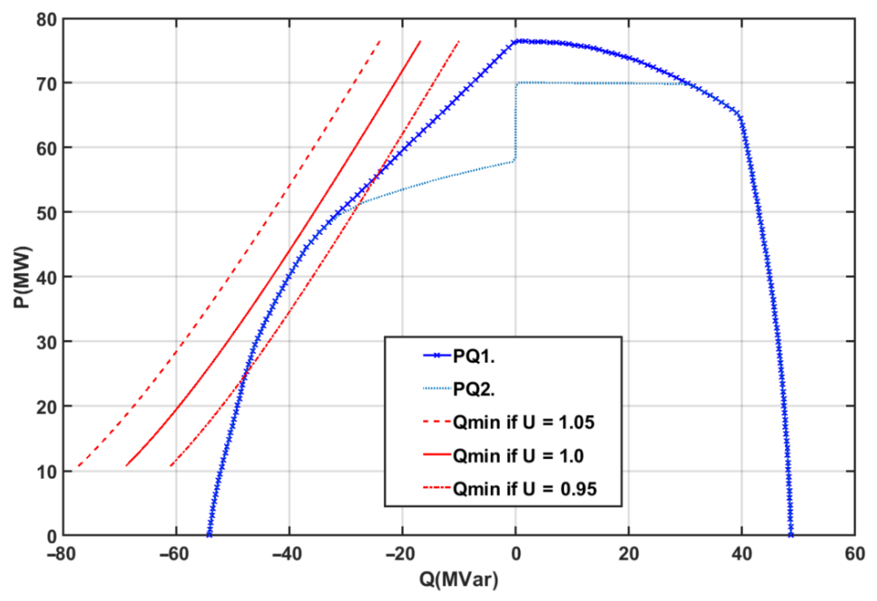
The Equations (22)–(24) form a system that can be analytically solved in real-time mode and thus determine the minimum value of reactive power for each power generation unit ensuring the steady-state stability (the input data: transfer direct-axis reactance $x_{d\mathsf{\Sigma }}$, HPP switchgear voltage level, turbine active power P_T, and the desired value of stability margin k_z).

Figure 6 shows P-Q diagrams of the renovated and non-renovated hydraulic units of the Novosibirsk HPP. It also depicts the minimum reactive power limits calculated using the expressions (22)–(24) under the conditions of parallel operation for the voltage range of 1.05–0.95 of the rated value. It is worth noting that for the rated voltage, the limitation curve lies to the left of the used P-Q diagrams. However, when the voltage on the high voltage busbars drops down to 0.95 of its rated value, the constraints according to the (22)–(24) should be used. In addition, the use of expressions (22)–(24) makes it possible to take into account different values of the steady-state stability margins and obtain a limiting line for the steady-state stability condition not only for a sole generator but taking into account the unit transformers. Furthermore, in the absence of the nameplate P-Q characteristics, the system of Equations (22)–(24) will allow designers and researchers to take into account the properties of salient-pole hydrogenators when carrying out power system studies using specialized software.

To test the proposed algorithms the authors performed simulations and assessed the correctness of the algorithms’ operation when power generation units were not uniformly loaded and were operated under conditions when some of the units had constraints on the apparent power and steady-state stability. The following data were analyzed during the tests:

• Active power P_i;
• Reactive load limit Q_min i;
• Given reactive power Q_i;
• Apparent power S_i.

After the uniform distribution algorithm was integrated into the digital AGC system of Novosibirsk HPP, the operation of the system was tested.

When individual control of unit No. 2 is implemented, the total reactive load is distributed equally between the units (Figure 7). In Figure 8, unit 2 has a lower value of the output reactive power. Additionally, automated field control cannot allow increasing the apparent power which can be seen by the warning indicator. The total value of the reactive load is distributed uniformly between the remaining units. In the case of reactive power consumption (Figure 9), unit 2 operates with the constraints on steady-state stability (24), and the rest of the units are uniformly loaded.

Based on the data obtained, it can be concluded that in the considered cases of the HPP operation, the uniform distribution algorithm operates without errors.

Table 3. Total active power losses observed at different values of Q_sum: Q_sum = 200 MVAr (dP_sum1) and Q_sum = −300 MVAr (dP_sum2).

dPsum	Proportional	Equality of Stator Current	Uniform
dPsum1, kW	2255.3	2255.6	2199.9
dPsum2, kW	3596.2	3511. 4	3511.4

presents the results of the calculations of the active losses occurring in the power plant electrical circuits.

When distributing the total reactive power of Q_sum = 200 MVar, the least active losses (dP_sum1) can be reached when using the uniform distribution, since it takes into account the criterion of active power loss minimization. In this case, the difference in active power losses for 5 hydroelectric units of the same type installed at Novosibirsk HPP is about 2.5%. In the case when the total reactive power setpoint is Q_sum = −300 MVar, both proposed distribution algorithms correspond to the same total active energy losses, since all the units operate with the steady-state stability constraints, which means that reactive power is distributed non-uniformly.

Based on the data obtained, it can be concluded that the uniform distribution algorithm is the optimal one due to its following advantages over the power distribution by equality of the stator currents:

• Less active power losses;
• The simplicity of the power distribution logic and calculations of constraints on apparent power and steady-state stability.

4. Conclusions

In the article, the issues of improving the automatic active power generation control of hydroelectric power plants are studied. The group active power control implies centralized control of the power generators as a single unit, which simplifies the participation of the HPP in the system-wide frequency and active power regulation. The process of group control is an extremely important part of the HPP control system as it regulates its main operating parameters: total active output power (within the daily dispatch schedule, etc.), and reactive power output. It also controls bus voltage levels and executes the tasks of automated load-frequency control. The article presents:

• The algorithm of active power distribution considers the individual control range of each of the hydraulic units and the head losses in the track rack. The algorithm also minimizes the total water discharge.
• The algorithm of reactive power distribution optimally minimizes the active power losses in the stator windings and the circuits of the unit transformers. The algorithm considers constraints on the apparent power, field current, and steady-state stability.
• An analytical expression is obtained for determining the minimum reactive power of a salient-pole generator that ensures its steady-state stability for the given value of the safety margin and the current values of the active power and voltage.
• The above algorithms and techniques are implemented in the digital AGC of the two hydropower plants.

References

1. Cutululis, N.A.; Farahmand, H.; Jaehnert, S.; Detlefsen, N.; Byriel, I.P.; Sørensen, P.E. Hydropower flexibility and transmission expansion to support integration of offshore wind. In Offshore Wind Farms: Technologies, Design and Operation, 1st ed.; Ng, C., Ran, L., Eds.; Woodhead Publishing: Sawston, UK, 2016; pp. 495–523. [Google Scholar]
2. Farahmand, H.; Jaehnert, S.; Aigner, T.; Huertes-Hernando, D. Nordic hydropower flexibility and transmission expansion to support integration of North European wind power. Wind Energy 2015, 18, 1075–1103. [Google Scholar] [CrossRef]
3. Matrenin, P.; Safaraliev, M.; Dmitriev, S.; Kokin, S.; Eshchanov, B.; Rusina, A. Adaptive ensemble models for medium-term forecasting of water inflow when planning electricity generation under climate change. Energy Rep. 2022, 8, 439–447. [Google Scholar] [CrossRef]
4. Khalyasmaa, A.; Eroshenko, S.; Bramm, A.; Tran, D.C.; Chakravarthi, T.P.; Hariprakash, R. Strategic planning of renewable energy sources implementation following the country-wide goals of energy sector development. In Proceedings of the International Conference on Smart Technologies in Computing, Electrical and Electronics, Bengaluru, India, 9–10 October 2020; pp. 433–438. [Google Scholar]
5. Mo, W.K.; Chen, Y.P.; Chen, H.Y.; Liu, Y.; Zhang, Y.; Hou, J.; Gao, Q.; Li, C. Analysis and Measures of Ultralow-Frequency Oscillations in a Large-Scale Hydropower Transmission System. IEEE J. Emerg. Sel. Top. Power Electron. 2018, 6, 1077–1085. [Google Scholar] [CrossRef]
6. Pico, H.V.; McCalley, J.D.; Angel, A.; Leon, R.; Castrillon, N.J. Analysis of very low frequency oscillations in hydro-dominant power systems using multi-unit modeling. IEEE Trans. Power Syst. 2012, 27, 1906–1915. [Google Scholar] [CrossRef]
7. Khalyasmaa, A.; Eroshenko, S.; Arestova, A.; Mitrofanov, S.; Rusina, A.; Kolesnikov, A. Integrating GIS technologies in hydro power plant cascade simulation model. E3S Web Conf. 2020, 191, 02006. [Google Scholar] [CrossRef]
8. Liu, Q.; Chen, G.; Liu, B.; Zhang, Y.; Liu, C.; Zeng, Z.; Fan, C.; Han, X. Emergency Control Strategy of Ultra-low Frequency Oscillations Based on WAMS. In Proceedings of the IEEE Innovative Smart Grid Technologies—Asia (ISGT Asia), Chengdu, China, 21–24 May 2019; pp. 296–301. [Google Scholar]
9. Nanda, J.; Kaul, B.L. Automatic generation control of an interconnected power system in Electrical Engineers. Proc. Inst. Electr. Eng. 1978, 125, 385–390. [Google Scholar] [CrossRef]
10. Kusic, G.L.; Sutterfield, J.A.; Caprez, A.R.; Haneline, J.; Bergman, B. Automatic generation control for hydro systems. IEEE Trans. Energy Convers. 1988, 3, 33–39. [Google Scholar] [CrossRef] [PubMed]
11. Kazantsev, Y.V.; Glazyrin, G.V.; Shayuk, S.M.; Tanfilyeva, D.; Tanfilyev, O.; Fyodorova, V. Hydro unit active power controller minimizing water hammer effect. In Proceedings of the IEEE Ural Smart Energy Conference (USEC), Ekaterinburg, Russia, 13–15 November 2020. [Google Scholar]
12. IEC 61362:2012; Guide to Specification of Hydraulic Turbine Governing Systems. 2012; p. 62. Available online: https://standards.iteh.ai/catalog/standards/iec/aa52f8df-d6ea-41dc-ac8c-1c03078ef02e/iec-61362-2012 (accessed on 12 September 2022).
13. Glazyrin, G.V.; Kazantsev, Y.V. Optimal control law for minimization of active power overshoot due to water hammer effect in a hydro unit. In Proceedings of the IEEE 11 International Forum on Strategic Technology (IFOST), Novosibirsk, Russia, 1–3 June 2016; pp. 329–333. [Google Scholar]
14. Campaner, R.; Chiandone, M.; Arcidiacono, V.; Milano, F.; Sulligoi, G. Automatic Voltage Control of a Cluster of Hydro Power Plants to Operate as a Virtual Power Plant. In Proceedings of the International Conference on Environment and Electrical Engineering (EEEIC), Rome, Italy, 10–13 June 2015. [Google Scholar]
15. Urin, V.D. Hydroelectric Plants Autoopearators Design Experience; Energoizdat: Moscow, Russia, 1969. [Google Scholar]
16. Manov, N.A.; Chukreev, Y.Y. Prototype of an expert system for dispatch adviser software in the regional power system. In New Information Technologies for Power System Dispatching; Ural Branch of the Russian Academy of Sciences: Ekaterinburg, Russia, 2002; pp. 43–59. [Google Scholar]
17. Mitrofanov, S.; Svetlichnaya, A.; Arestova, A.; Rusina, A. Development of a Software Module of Intra-Plant Optimization for Short-Term Forecasting of Hydropower Plant Operating Conditions. In Proceedings of the IEEE Ural-Siberian Smart Energy Conference (USSEC), Novosibirsk, Russia, 13–15 November 2021. [Google Scholar]
18. Gaidukov, J.; Glazyrin, G.; Glazyrin, V.; Eroshenko, S. Control algorithms and optimization method of the hydroelectric power plant’s microprocessing joint power control. In Proceedings of the 2020 Ural Smart Energy Conference, Ekaterinburg, Russia, 13–15 November 2020; p. 9281275. [Google Scholar]
19. Alterman, D.Z. Hydroelectric Plants Autocontrol Systems with Active Power Correction; Energoizdat: Moscow, Russia, 1959. [Google Scholar]
20. Kiselev, G.S. The experience of serial microcontroller application to hydro unit automation. Energetik 1998, 4, 37–45. [Google Scholar]
21. Muraviev, O.A.; Berlin, V.V. The experience of setup up of group control of active power of Kureiskaya hydroelectric plant. Proc. MSSU 2001, 1, 107–114. [Google Scholar]
22. Garcia, D.J.; Loreto, J.L. Automatic generation control of the caruachi hydro-electric power plant. In Proceedings of the IEEE Transmission and Distribution Conference and Exposition, Caracas, Venezuela, 15–18 August 2006. [Google Scholar]
23. Lansberry, J.E.; Wozniak, L. Adaptive hydrogenerator governor tuning with a genetic algorithm. IEEE Trans. Energy Convers. 1994, 9, 179–183. [Google Scholar] [CrossRef]
24. Rusina, A.G.; Sovban, E.A.; Khujasaidov, J.K.; Filippova, T.A. Tasks of optimal performance of hydroelectric in power system. In Proceedings of the 11th International Forum on Strategic Technology (IFOST), Novosibirsk, Russia, 1–3 June 2016. [Google Scholar]
25. Liu, S.L.; Song, Y.X.; Hao, P.L. The Fuzzy Comprehensive Evaluation of Hydropower Plant Production and Operating Conditions Based on the BP Neural Network Improved. Appl. Mech. Mater. 2011, 71–78, 4170–4173. [Google Scholar]
26. Liu, B.; Liao, S.; Cheng, C.; Wu, X. Multi-Core Parallel Genetic Algorithm for the Long-Term Optimal Operation of Large-Scale Hydropower Systems. In Proceedings of the World Environmental and Water Resources Congress, West Palm Beach, FL, USA, 22–26 May 2016; pp. 220–230. [Google Scholar]
27. Robert, Q.; Planque, J.L. Robust Digital Automatic Reactive Power Regulator for Hydro Power Plants. In Proceedings of the 2007 International Conference on Clean Electrical Power, Capri, Italy, 21–23 May 2007; pp. 175–179. [Google Scholar]
28. Arce, A.; Ohishi, T.; Soares, S. Optimal Dispatch of Generating Units of the Itaipú Hydroelectric Plant. IEEE Trans. Power Syst. 2002, 17, 154–158. [Google Scholar] [CrossRef]
29. Sheble, G.B.; Fahd, G.N. Unit Commitment Literature Synopsis. IEEE Trans. Power Syst. 1994, 9, 128–135. [Google Scholar] [CrossRef]
30. Byrd, R.H.; Gilbert, J.C.; Nocedal, J. A Trust Region Method Based on Interior Point Techniques for Nonlinear Programming. Math. Program. 2000, 89, 149–185. [Google Scholar] [CrossRef] [Green Version]
31. Byrd, R.H.; Hribar, M.E.; Nocedal, J. An Interior Point Algorithm for Large-Scale Nonlinear Programming. SIAM J. Optim. 1999, 9, 877–900. [Google Scholar] [CrossRef]
32. Waltz, R.A.; Morales, J.L.; Nocedal, J.; Orban, D. An interior algorithm for nonlinear optimization that combines line search and trust region steps. Math. Program. 2006, 107, 391–408. [Google Scholar] [CrossRef]
33. Zhao, X.; Yang, Y.; Wei, H. An interior point method based on continuous Newton’s method for optimal power flow. In Proceedings of the IEEE PES Innovative Smart Grid Technologies, Tianjin, China, 21–24 May 2012. [Google Scholar]
34. Jie, Z.; Shengchun, L.; Yao, R.; Liang, D.; Zhanshan, Y.; Yongfei, M. Reactive power optimization for AVC system based on decoupled interior point method. In Proceedings of the 2022 14th International Conference on Measuring Technology and Mechatronics Automation (ICMTMA), Changsha, China, 15–16 January 2022; pp. 131–133. [Google Scholar]
35. Wang, Y.; Jiang, Q. Reactive power optimizatin of distribution network based on primal-dual interior point method and simplified branch and bound method. In Proceedings of the 2014 IEEE PES T&D Conference and Exposition, Chicago, IL, USA, 14–17 April 2014. [Google Scholar]
36. Rojas, D.G.; Lezama, J.L.; Villa, W. Metaheuristic Techniques Applied to the Optimal Reactive Power Dispatch: A Review. IEEE Lat. Am. Trans. 2016, 14, 2253–2263. [Google Scholar] [CrossRef]
37. Saka, B.; Aibinu, A.M.; Mohammed, Y.S.; Olatunji, D.E. Voltage Stability of the Power System using Genetic Algorithm: A Review. In Proceedings of the 2021 1st International Conference on Multidisciplinary Engineering and Applied Science (ICMEAS), Abuja, Nigeria, 15–16 July 2021. [Google Scholar]
38. Steihaug, T. The Conjugate Gradient Method and Trust Regions in Large Scale Optimization. SIAM J. Numer. Anal. 1983, 20, 626–637. [Google Scholar] [CrossRef] [Green Version]
39. Brent, R. Algorithms for Minimization Without Derivatives; Prentice-Hall: Hoboken, NJ, USA, 1973. [Google Scholar]
40. Kundur, P. Power System Stability and Control; McGraw-Hill: New York, NY, USA, 1994. [Google Scholar]
41. Jackson, J.Y. Interpretation and Use of Generator Reactive Capability Diagrams. IEEE Trans. Ind. Gen. Appl. 1971, IGA-7, 729–732. [Google Scholar] [CrossRef]
42. El-Kady, M.A.; Bell, B.D.; Carvalho, V.F.; Burchett, R.C.; Happ, H.H.; Vierath, D.R. Assessment of Real-Time Optimal Voltage Control. IEEE Trans. Power Syst. 1986, PWRS-1, 98–107. [Google Scholar] [CrossRef]
Figure 1. HPP units’ efficiency at different water heads.
Mathematics 10 04809 g001
Figure 2. Water discharge for the HPP having 3 hydraulic units and a power output setpoint of 90 MW (PU3 is calculated using Equation (7) for the given load schedule PS).
Mathematics 10 04809 g002
Figure 3. The flowchart of the algorithm for optimal power distribution on the criterion of equality of incremental turbine discharges with consideration of head losses in a trash rack.
Mathematics 10 04809 g003
Figure 4. Power-angle curves for salient pole synchronous machines.
Mathematics 10 04809 g004
Figure 5. Incremental water discharge versus turbine power graphs for hydraulic units of Novosibirsk HPP and the solution of the Equation (17).
Mathematics 10 04809 g005
Figure 6. P-Q capability diagram of Novosibirsk HPP hydroelectric generator.
Mathematics 10 04809 g006
Figure 7. The main window of the digital AGC system: unit 2 individual control is active.
Mathematics 10 04809 g007
Figure 8. The main window of the digital AGC system: unit 2 has constraints on apparent power.
Mathematics 10 04809 g008
Figure 9. The main window of the digital AGC system: unit 2 has constraints on steady-state stability.
Mathematics 10 04809 g009