In this section, we present a way to modify the seed model to move or remove faulty relationships and add missing relationships to the model. Here, the meaning of moving an erroneous relationship is to attach the relationship to a node in the graph. We propose two approaches to remove or move potentially incorrect relationships. First, we use machine learning techniques to distinguish some ambiguous relationships based on the data source. Then, some incorrect substructures of cm can be detected through matching model fragments in a knowledge graph. After removing or moving incorrect relationships, we add potentially missing substructures of cm by using a modified frequent subgraph mining algorithm. As a result, a high-quality semantic model is obtained.
4.2.1. Move Incorrect Relationships
One entity may be linked to multiple other entities by various relationships. For example, the entity
E52_Time-Span can be linked with
E12_Production,
E8_Acquisition,
E67_Birth, and
E69_Death by relationship
P4_has_time-span in the gold semantic models of the
museum-crm dataset. We define such an entity as an ambiguous entity and the attributes it labeled as ambiguous attributes. In the candidate model generated by the Steiner Tree algorithm, some elements may be wrong because of multiple possible relationships. For example, as
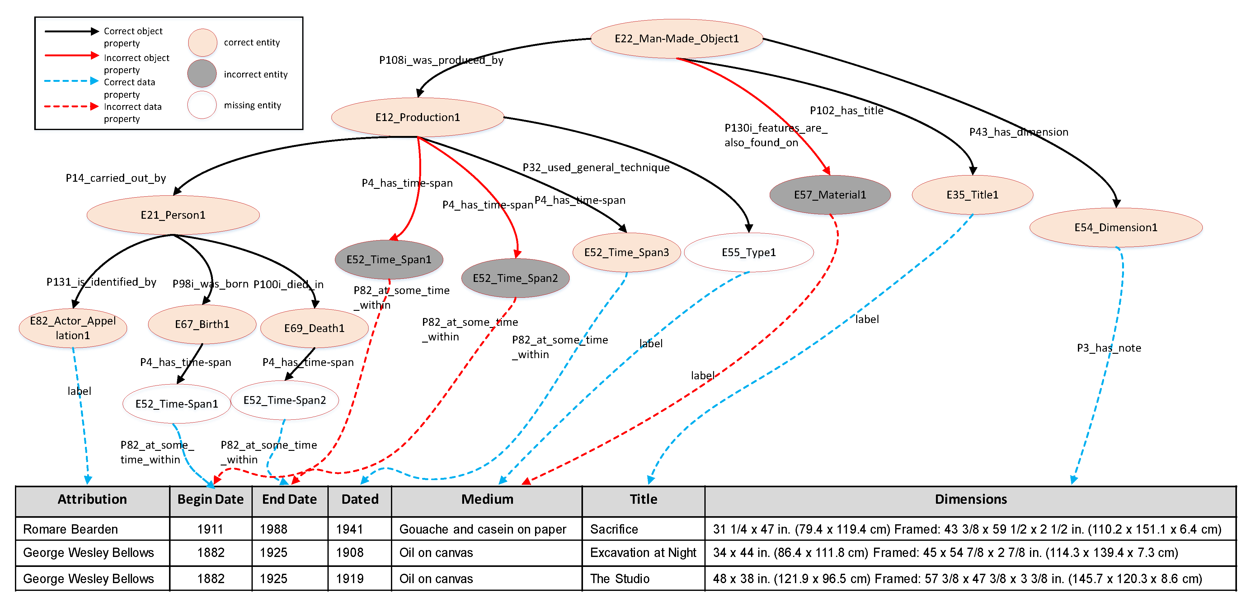
Figure 3 shows, the relationships
P4_has_time-span from the entity
E12_Production to
E52_Time-Span2 and
E52_Time-Span3 are incorrect. In fact, these entities should be linked with
E67_Birth and
E69_Death by relationship
P4_has_time-span respectively. In this section, we put forward a machine learning method to move such ambiguous relationships. We treat the problem of distinguishing ambiguous relationships as a multi-category classification problem. Similarity metrics are used as features of the learning matched function to determine whether different ambiguous attributes have the same relationship and thereby infer the correct links.
Our method of removing incorrect relationships is summarized in the following: (1) For training data sources, we gather all ambiguous attributes (their corresponding ambiguous relationships are known), extract several features and train a decision tree model [
27]; (2) For a new data source, we find all the ambiguous attributes and use the trained decision tree model to determine the correct linking position; and (3) We move the relationships according to the predicted result.
We used the following candidate features, including attribute name similarity, value similarity, distribution similarity, and histogram similarity to a decision tree model. Besides these, we also use an external
knowledge base to generate additional features. We briefly describe these similarities in the following: (1) Attribute Name Similarity: Usually, there is a
title for each column of a structural tabular data source such as a Web table or spreadsheet. We treat these headings as attribute names and use them to compare the similarities between attribute names and entity names. The similarity may infer the correct relationship to which the entity is linked. For example, if an attribute is named
birthDate, its labeled entity should be
E52_Time-Span link with entity
E67_Birth rather than entity
E69_Death. (2) Value Similarity: Value similarity is the most commonly used similarity measure, which has been used in various matching systems. Since the same semantic types usually contain similar values, value similarity plays a significant role in recognizing attributes labeled by the identical semantic types. In our method, two different value similarity metrics are applied, i.e., Jaccard similarity [
28] and TF-IDF cosine similarity [
28] for computing the value similarity of textual data. (3) Distribution Similarity: For numeric data, value similarity is always ineffective to distinguish semantic types because they always have the similar value range. However, their distribution of values may be different because they have different potential meanings. Therefore, we use statistical hypothesis testing as one of the similarity measures to analyze the distribution of values in attributes. We also used the Kolmogorov–Smirnov test (KS test) [
29] as one of the similarity metrics. (4) Histogram Similarity: Histogram similarity calculates value histograms in textual attributes and compares their histograms. The statistical hypothesis test for the histograms is the Mann–Whitney test (MW test) [
29]. In our method, the MW test is used for computing the histogram similarity, considering it calculates the distribution distance based on medians. (5) External Knowledge Base: To improve the accuracy of our approach further, we used an external knowledge base as a candidate feature. In the cultural heritage community, the Getty Union List of Artist Names (ULAN)
https://www.getty.edu/research/tools/vocabularies/ulan (14 December 2022) is an authoritative reference dataset containing over 650,000 names of over 160,000 artists. For the museum datasets, some ambiguous attributes can be distinguished by retrieving the information from ULAN. For example, we can validate the information of biography of artists by comparing the information with an attribute labeled by
E52_Time-Span with ULAN to determine if the information with
E52_Time-Span really represents the birth date of artists.
Our approach to distinguishing ambiguous attributes is stated in detail as follows. Given an ambiguous entity, where the number of possible links is
, we randomly select
k attributes {
,
, ...,
} from the training attributes as reference attributes. The reference attributes should contain all possible relationships. For other training attributes {
,
,
, ...
}, we compute multidimensional feature vectors
by comparing against all reference attributes and searching the external knowledge base. During training, we label each
as a number
j (ranging from 1 to
k), where
j means the
possible relationships. Given a new ambiguous attribute
, we compute the feature
and use the learned tree model to label
as a number ranging from 1 to
k. Unlike [
22], for each attribute, we compute only one feature vector by comparing it with all the reference attributes. If the label of
is
m, it means that
is linked by the
possible relationships. If the predicted result is not consistent with the relationship in the seed model, we move the relationship according to the predicted result.
For the seed model of CB, as
Figure 3 shows, the corresponding relationships of ambiguous attributes
Begin Date, and
Death Date are (
E12_Production,
P4_has_time-span,
E52_Time-Span). These are wrong predictions by the Steiner Tree algorithm.
Figure 4 shows the changes after moving the ambiguous relationships. Through our method, the correct relationships of these attributes can be predicted, and the incorrect relationships are moved into the correct linking position, i.e., (
E67_Birth,
P4_has_time-span ,
E52_Time-Span1) for
Begin Date and (
E69_Death,
P4_has_time-span,
E52_Time-Span2) for
End Date.
4.2.3. Add Missing Substructures
In the seed model, some relationships may be missing. To enhance the integrity of the seed model, we need to add extra substructures. Note that there must exist data types in the data source that the added substructures can match. For instance, as shown in
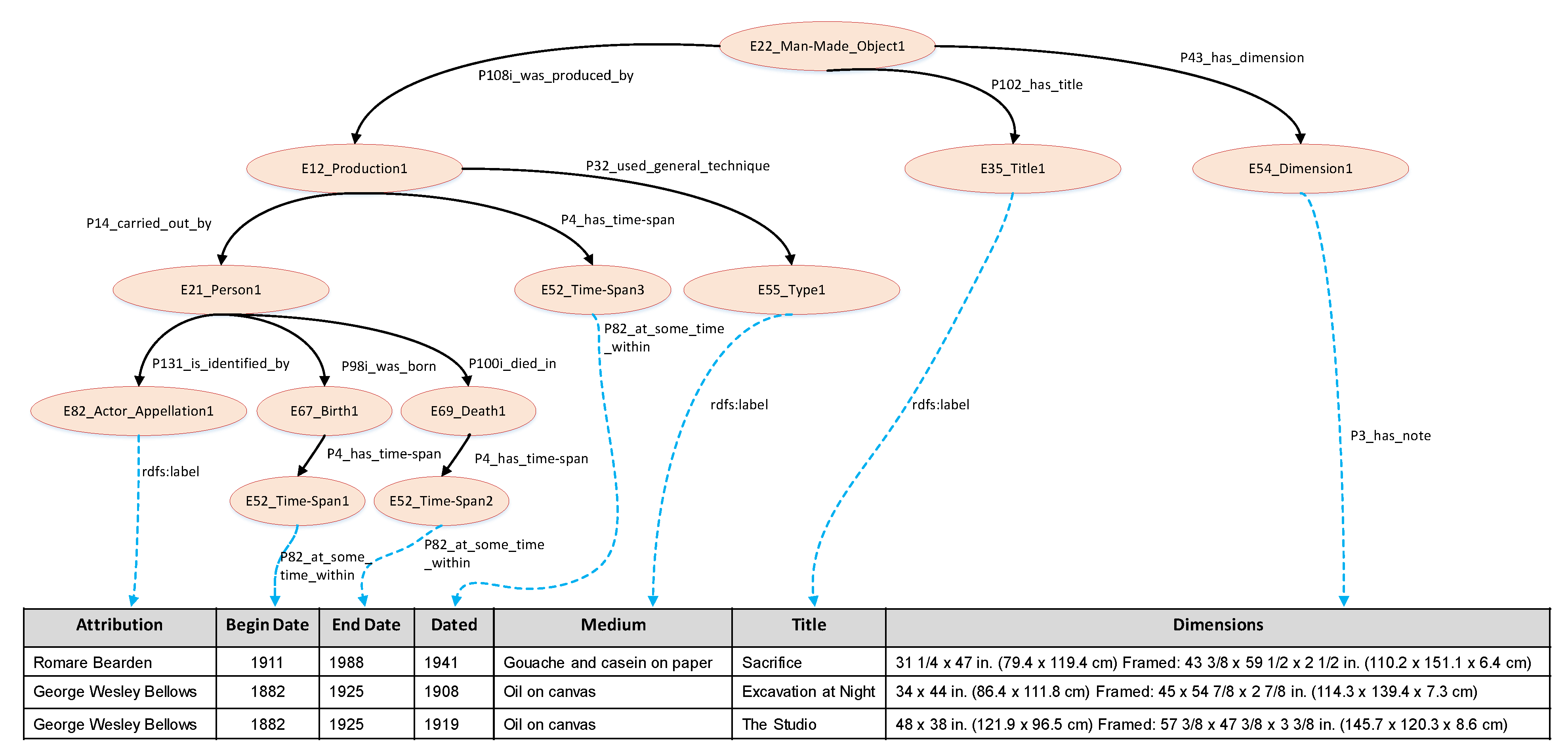
Figure 1, if some attributes in the data are date or time matching
E67_Birth1, it may be reasonable to amend the model and choose entity
E52_Time-Span1 to match these attributes.
Each column of the new data source may correspond to several candidate semantic types, and every semantic type has an ascribed confidence score computed during the initial semantic labeling step. However, the semantic type with the highest confidence score may not capture the correct semantics of the source attribute. For example, the correct semantic type of column Medium of data source CB is E55_Type, while its first learned semantic type is E57_Material. Accordingly, we consider multiple candidate semantic types for each column of the source when semantic models are constructed.
Considering multiple semantic types may make our method less efficient in constructing a semantic model of a source. Hence, we apply several
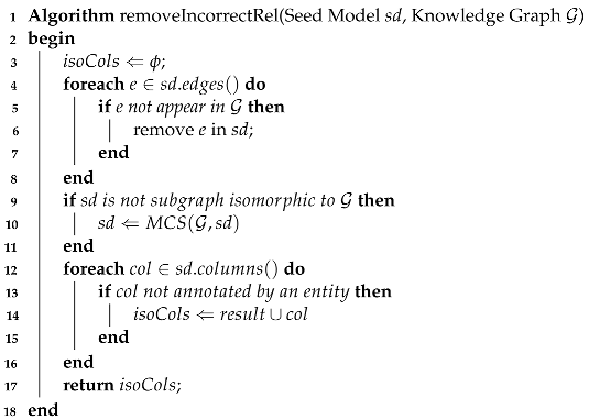
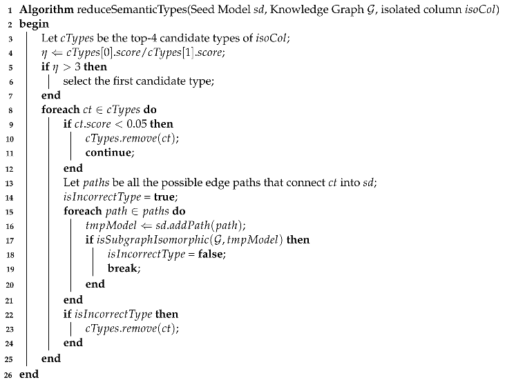
heuristics to increase the effectiveness of our method in our algorithm. Algorithm 2 is used to check and reduce candidate semantic types of an isolated column based on their confidence score and a knowledge graph. First, we denote
as the ratio between the confidence score of the first ranked candidate type and the second candidate type (Line 4). However,
might not be preset high enough to avoid the consideration of too many candidate semantic types. We empirically set three as the threshold value of
based on the experimental results in
Table 1. If
is larger than three, we only select the first candidate type as the final candidate type (Lines 5–8). Second, we remove all the candidate types whose confidence scores are lower than 0.05 of a column (Lines 10–13). Finally, some candidate semantic types with high confidence scores can be quickly excluded by searching within the knowledge graph using the subgraph matching technique. For the candidate semantic type
with a relatively high confidence score (larger than 0.05), we attempted to search all the paths
in
that connect
into candidate model
after removing a presumed incorrect edge. If no such graph connecting a path in
into
is subgraph-isomorphic to the knowledge graph, we remove this candidate type (Lines 14–25). A VF2 algorithm [
31] is used for checking subgraph isomorphism. This process aims to find the entities in
that do not co-occur with other substructures in the knowledge graph. If such entities are considered as candidate semantic types, the frequent subgraph mining algorithm may return none of the resulting models while costing much time. After running Algorithm 2, some candidate types are removed, which prunes large portions of the search space.
| Algorithm 2: Algorithm of reducing candidate semantic types for an isolated column. |
![Mathematics 10 04778 i002 Mathematics 10 04778 i002]() |
In the seed model of CB, for the isolated column Medium, the confidence scores of the last two candidate semantic types are lower than 0.05, so we filter them out in candidate types. For the incorrect type E57_Material of attribute Medium, there is only one possible relationship connecting it into , i.e., (E22_Man-Made_Object, P45_consists_of, E57_Material). However, if we try to add this relationship in , we find the intermediate model is not subgraph-isomorphic to . So the candidate semantic type E57_Material might be incorrect, and we can eliminate it from consideration. After reducing the candidate semantic types, there is only one candidate semantic type i.e., E55_Type1 for the column Medium.
Algorithm
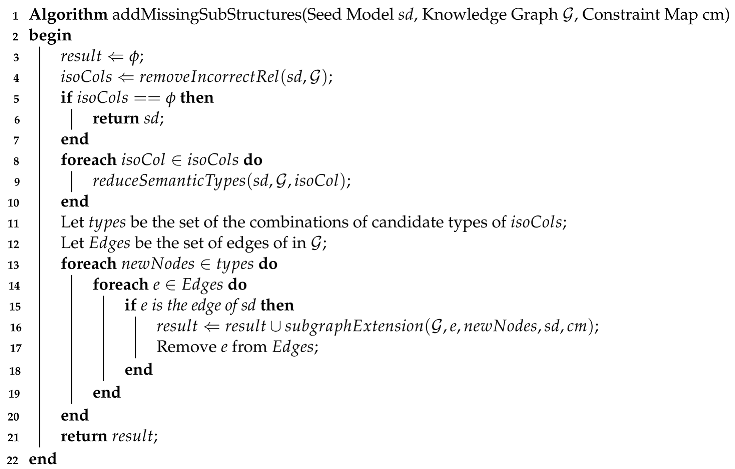
addMissingSubStructures (Algorithm 3) is proposed to search and add deleted substructures of imperfect seed semantic model
sd. First, we use Algorithm 1 to remove incorrect substructures and obtain
of
(Line 4). If the attribute set
is empty, the algorithm returns
as the result (Lines 5–7). In this case, none of the incorrect relationships is detected by Algorithm 1. The seed model might be the correct model. Then, we iterate over the set
, and for each attribute
, we use Algorithm 2 to reduce its candidate semantic types (Lines 8–10). After these steps, we enumerate all the possible combinations of candidate semantic types of
and run the modified frequent subgraph mining algorithm (Lines 13–21). Unlike the traditional algorithm, we abandon the parameter frequency threshold
for the uncertainty of the frequency threshold of the correct model. Without the limitation on frequency, the efficiency of frequent subgraph mining algorithms may decrease. Accordingly, we propose a set of pruning strategies for speeding up our algorithm. These pruning strategies will be introduced below. The output of Algorithm 3 is the set
, which stores all frequent subgraphs as complementary semantic models.
| Algorithm 3: Algorithm for repairing the seed model. |
![Mathematics 10 04778 i003 Mathematics 10 04778 i003]() |
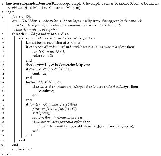
As the sub-function of Algorithm 3, Algorithm
subgraphExtension (Algorithm 4) is used to search and add missing substructures from a specific imperfect semantic model
. The inputs of Algorithm 4 are a seed model
sd, a knowledge graph
, an incomplete semantic model
, a constraint map cm, and the candidate semantic types
that the seed model may link with. The
grow-and-store strategy is adopted in the algorithm
subgraphExtension for recursively mining the top-
frequent subgraphs of
. In the meantime, Algorithm 3 can ensure the coverage between the seed model
sd and all of the candidate semantic types
of source attributes in the mined top-
frequent substructures. Here, our
heuristic is that if the frequency of an amended semantic model is higher than a certain threshold in the knowledge graph, it indicates that the model could be correct. Further, the higher the frequency of an amended model in the knowledge graph, the more likely it is to be a reasonable semantic model. The output of the algorithm
subGraphExtension is the top-
semantic models with complemented missing substructures.
| Algorithm 4: Algorithm of subgraph extension. |
![Mathematics 10 04778 i004 Mathematics 10 04778 i004]() |
The inputs of Algorithm 4 are illustrated as below.
Semantic Labels is a candidate combination of candidate semantic types of the source attributes that does not occur in the seed model of a new data source.
Constraint Map is a HashMap which constraints the maximum count of entities for each semantic type that may appear in a correct model. Generally,
Constraint Map is prescribed through domain expertise. For instance, as
Figure 1 shows, in the semantic model of the CB, the
Constraint Map limits the count of entities for the semantic types
E52_Time-Span, and
E35_Title must be less than three and one, respectively. The intermediate variable
is a sorted integer list used to record the top-
frequencies of all subgraphs throughout the algorithm process.
For each relationship e in knowledge graph and a semantic type n in the incomplete model , first Algorithm 4 validated if e can be linked with the semantic type n and whether e is a valid edge in the knowledge graph (Line 6). For instance, assume that entities E22_Man-Made_Object1 and E35_Title1 and a relationship P102_has_title occur in an initial subgraph. Suppose n is semantic type E22_Man-Made_Object1 in S and e is object property P43_has_dimension. Since contains the triple (E22_Man-Made_Object1, P43_has_dimension, E54_Dimension1), it implies that P43_has_dimension is effective and can be used to link with E22_Man-Made-Object1. Let be the extension of with e (Line 7). During the run of Algorithm 4, when all the nodes and links in the seed model and candidate semantic types are covered in , the is the most possibly plausible semantic model which correctly captures the semantics of the data source. Next, is merged into the set , and the algorithm ceases and returns (Lines 8–11). The set is used to store the top- semantic models as the output of the algorithm subGraphExtension. As Algorithm 3 demonstrates, the set represents one possible combination of all candidate semantic types of , may be erroneous to annotate semantic types for . Algorithm 4 may return none, which indicates that there are some incorrect candidate types in the .
We apply some pruning strategies to improve the efficiency of the algorithm. In order to prevent the recurrence of a given entity type in the model, one of the pruning strategies we employ is to leverage Constraint Map to limit the searching space. We check each entity in Constraint Map cm. If there is an entity type that appears in exceeding times, the further search for current is ceased (Lines 13–15). The Function count() is used to calculate the number of appearances of in the intermediate subgraph .
We reduce the search space by leveraging the structure of . We iterate over the edge of , and if there is an edge e whose source node and target node exist in but e does not exist in , we stop searching (Lines 16–20). For example, in the seed model of CB, entity E22_Man-Made_Object and entity E12_Production are connected by relationship P108i_was_produced_by. For an intermediate substructure containing these entities, if there is no link between the two entities, can not be extended to the model which contains the relationship P108i_was_produced_by. It is vain to further search substructure . In practice, a large amount of search space can be reduced by using this pruning strategy. For the seed model of CB, the running time is about 15 s, while without this optimization, the respective running time is about 5 min.
Next, we use a Minimum Image-based Metric based on a subgraph matching algorithm [
32] (Line 21) in the function
to calculate the frequencies of
occurring in
G. All the substructure
in which the frequency is lower than the minimum frequency of
will be discarded. The intuition behind this pruning strategy is that the correct semantic model may be a subgraph with higher frequency in the knowledge graph. During the process of search, only the top-
frequent subgraphs are retained as candidate semantic models in the frequency-based pruning strategy.
In Algorithm 4, during the whole search, top- frequencies of all subgraphs are stored in an integer list (line 22) in which the length is . Here, merges the frequency of () (Line 22) if the frequency of is higher than the minimum value of the current . Then, Algorithm 4 sorts (Line 23) and removes the minimum value in the sorted (Line 24).
Thereafter, for removing duplicate models, Algorithm 4 checks if
has been searched in the previous procedure. We exploit the
canonical code method proposed in [
14] to detect the duplicate models (Line 25). The algorithm
subgraphExtension is recursively executed (Line 26) for further search if the substructure
has not been generated before.
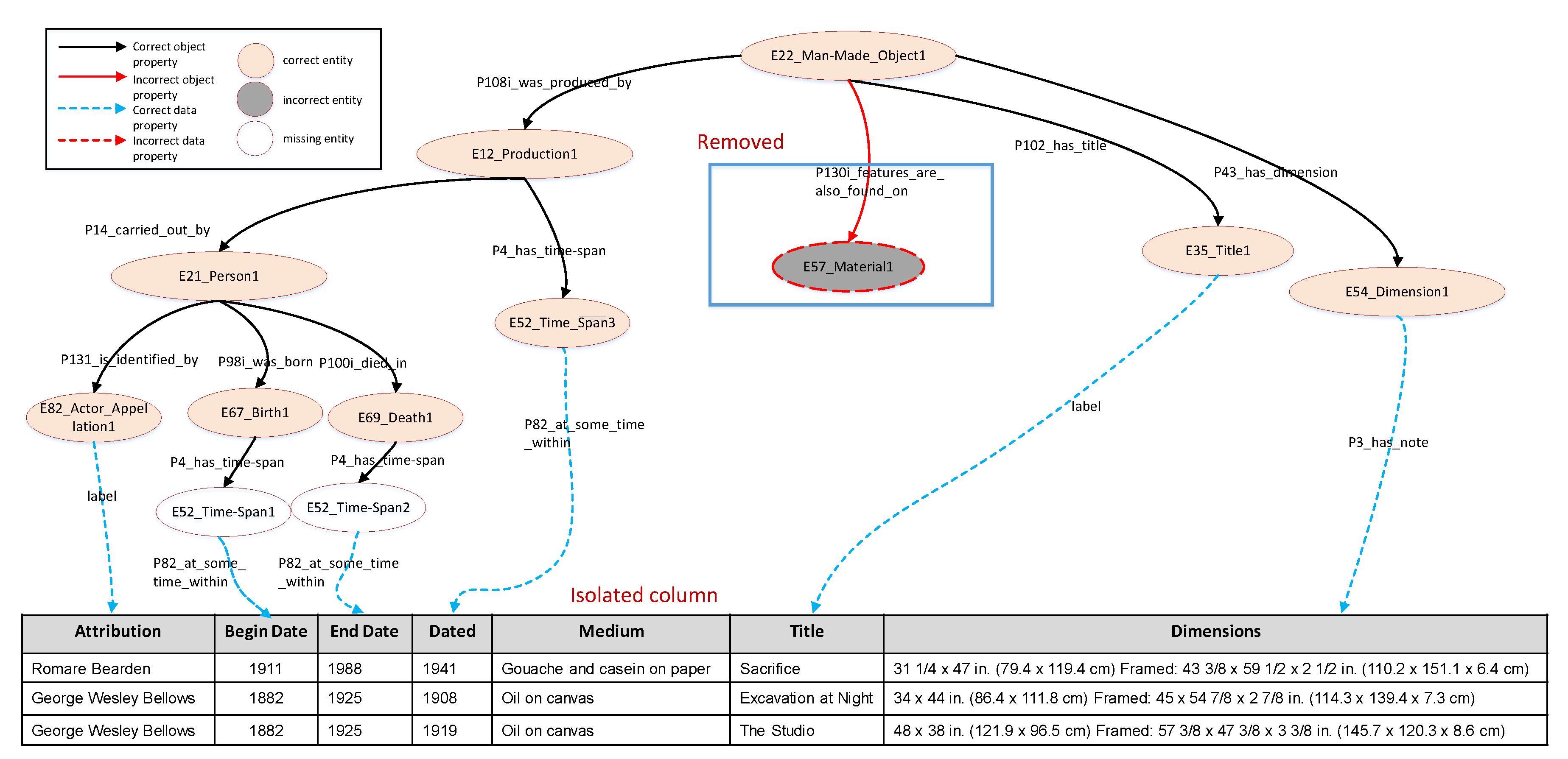
The incomplete model of CB before adding missing substructures is shown in
Figure 5 (wrong entity
E57_Material1 and its relationship were removed). After reducing the candidate semantic types,
E55_Type1 is the only candidate type for isolated column
Medium. Through the process of our modified subgraph mining algorithm, the missing relations (
E12_Productioin1,
P32_used_general_technique,
E55_Type1) can be linked into the incomplete model, and the gold standard model (
Figure 1) can be output as a frequent subgraph. Hence, the seed model of CB is amended into a correct semantic model.
