Abstract
Volumetric images have a three-dimensional (3D) view, in which viewers can examine their characteristics from any angle. The more accurate the digital representation of volumetric images, the more precise and valuable the assessment of what these images represent. The representation of volumetric images is a significant area of study in pattern recognition and computer vision. Recently, volumetric image analysis using orthogonal moments with fractional order has opened up a new study pathway, which has led scholars to discover many real-life applications through investigating efficient algorithms to represent the features of 3D images. In this study, a new set of 3D shifted fractional-order Gegenbauer moments (FrGMs) for volumetric image representation is proposed. First, a mathematical description of the shifted Gegenbauer moments for 3D images is presented. Second, a fast, highly accurate method for calculating the fractional-order shifted Gegenbauer moments of 3D images is introduced. Finally, the efficiency of the proposed FrGMs is evaluated through various suitable experiments and compared with existing methods in terms of the reconstruction of 3D images, the invariability property, sensitivity to noise, and computation time. The experimental results clearly show that FrGMs outperform existing related algorithms.
Keywords:
fractional-order orthogonal moments; shifted Gegenbauer polynomials; fast and accurate computation; 3D image representation MSC:
68U10; 68U05
1. Introduction
Due to their ability to describe an image’s content, the moments of an image are considered the most useful transformations of image processing. Image moments are effective invariant features that have been widely exploited in various image processing applications in recent years [1,2,3].
Teague [4] proposed the use of orthogonal moments (OMs) in a continuous domain to describe an image with no need for information redundancy or noise resistance due to the orthogonality property. As demonstrated by Papakostas [5] and Flusser et al. [6], OMs also have the property of representing two-dimensional (2D)/three-dimensional (3D) images with minimal information redundancy, which is useful in a variety of applications.
There has been tremendous advancement in 3D model acquisition technology, and 3D images are gaining popularity, as the description and representation of 3D features and 3D image/object reconstruction are essential for various scientific fields. With the advancement of technology, science, and industry, 3D images are becoming increasingly useful in medical imaging, bioengineering, reverse engineering, computer-aided design, and industrial production [7,8,9]. Three-dimensional laser scanners play an essential role in reverse engineering. Laser-based sensors are fast, non-contact, and therefore commonly used to digitize objects [10]. For example, in medical imaging, using computed tomography (CT) or magnetic resonance imaging (MRI) scanners, a regular volumetric grid with a volume element/voxel is represented by a single value obtained by sampling the immediate area surrounding the voxel.
Alternatively, a 3D dataset can be represented as a group of 2D slice images [11]. In computer vision, the orthogonal transforms and functions used in constructing OMs are important image descriptors for extracting essential features from 2D/3D images. Research on moments and moment invariants has grown increasingly in 3D image analysis, with numerous applications. Based on the algebraic properties of Krawtchouk polynomials, Benouini et al. [12] introduced direct Krawtchouk moment invariants, an efficient set of moment invariants for 3D recognition. Kumar [13] used 3D geometric moments to extract features and applied them to hyperspectral image classification. Karmouni et al. [14] introduced a fast reconstruction of a 3D image by combining discrete Charlier moments and cuboids. Based on CT and MRI measurement and the analysis of the femoral condyle torsion angle, Yang et al. [15] built a joint model of a 3D digital knee.
Karmouni et al. [16] proposed a 3D image classification method based on a quick computation of 3D Meixner invariant moments using a 3D image cuboid representation, which could greatly reduce the time required in the computation process.
Tahiri et al. [17] introduced a novel set of hybrid polynomials and their related moments with the goal of using them to localize, compress, and reconstruct large 2D/3D images. Sayyouri et al. [18] presented an accurate and fast calculation algorithm for generalized fractional-order Laguerre OMs computed in the Cartesian coordinate. These moments were also applicable to the invariant recognition or reconstruction of 2D/3D images. Hosny [19] introduced fast and exact methods for calculating 3D Legendre moments, in which scale and translation invariance are constructed directly using exact 3D central Legendre moments. These moments are used in the reconstruction and description of large 3D images/objects.
Karmouni et al. [20] proposed an efficient and fast approach for calculating the 3D discrete orthogonal invariant moments of Meixner, Krawtchouk, Tchebichef, Hahn, and Charlier of 3D images applicable to 3D image classification. Sit et al. [21] created a new set of local descriptors called 3D Krawtchouk descriptors for identifying and comparing the local protein regions of 3D voxelization-oriented surfaces. Jahid et al. [22] proposed a new efficient and fast algorithm for computing orthogonal Meixner moments on discrete 3D images based on a new 3D image representation using cuboids with the same gray levels, called image cuboid representation. Yamni et al. [23] introduced a new rapid and accurate approach for computing Meixner moments for 2D/3D image classification. These moments have the potential to be useful feature descriptors for 2D/3D object recognition.
Rivera-Lopez et al. [24] introduced a fast and efficient method for computing 3D Tchebichef moments for higher orders by combining advantage parallelization with the Kronecker tensor product. These 3D Tchebichef moments for higher orders are vital tools for the analysis and characterization of 3D objects. By introducing image moments as an input layer in deep neural networks (DNNs), Lakhili et al. [25] proposed a new model based on 3D discrete OMs and DNNs to improve the classification accuracy of 3D objects. Yamni et al. [26] proposed an accurate and fast method for computing 3D Charlier moment invariants for 3D image classification.
A new set of separable discrete moments, Tchebichef–Tchebichef–Krawtchouk moments and Tchebichef–Krawtchouk–Krawtchouk moments, was introduced by Batioua et al. [27] for 3D image analysis. Zouhir et al. [28] introduced a new model for 3D shape classification named 3D Hahn moments neural networks (3DHMNNs) to decrease the computational complexity and improve the classification accuracy of 3D pattern recognition process.
In these studies, the OMs were defined for integer order, in which the corresponding order of the OMs was an integer. Recently, scientists [29,30,31,32] have proven that OMs with fractional orders outperform their corresponding moments of integer orders. Therefore, researchers are interested in fractional-order OMs. Several applications of fractional-order OMs have recently been discovered through research, such as image analysis, pattern recognition, copy–move image forgery, image reconstruction, watermarking of biomedical signals and images, plant disease recognition, color face recognition, robust and zero-watermarking of digital images, and color image encryption [33,34,35,36,37,38,39,40,41,42,43,44,45,46,47,48].
Most published works on continuous fractional-order OMs have been shown to represent 2D images. However, constructing fractional-order OMs for 3D image analysis has received little attention. El Ogri et al. [49] defined generalized fractional-order Laguerre functions and introduced new sets of 3D fractional-order generalized Laguerre moments (FrGLMs). El Ogri et al. [50] introduced fractional-order orthogonal Legendre moments (FrOLMs) and applied them in the description and recognition of 3D objects.
A successful description of scanned 3D medical data requires accurate 3D descriptors. Traditional 3D descriptors suffer from two kinds of errors: geometric and numerical. Geometric errors are the result of image mapping in which the scanned data and the basic functions of the descriptors are defined in different coordinates. Numerical errors result from inaccurate computation or approximation of the image descriptors. These errors significantly reduce the ability of descriptors to represent 3D images.
This study presented a new set of shifted fractional-order Gegenbauer moments (FrGMs) defined in the Cartesian domain and directly utilized without any mapping to represent 3D images. The proposed descriptors completely removed geometric errors and minimized numerical errors.
This study makes the following contributions:
- We defined a new set of 3D shifted fractional-order Gegenbauer moments (3D FrGMs).
- Image mapping was not required, as both standard 3D images and the 3D shifted Gegenbauer moments were defined on a unit cube .
- As indicated in point 2, we completely removed the source of the geometric errors.
- A highly accurate computational method was used to compute the 3D FrGMs, minimizing numerical errors.
The rest of this paper is organized as follows. The second section presents a brief description of the FrGMs for 2D images. The third section discusses the proposed 3D FrGMs for 3D images and shows the accurate and fast computation of the FrGMs for 3D images. The fourth section presents the experimental results. The fifth section provides the conclusion.
2. Overview of 2D FrGMs
This section provides an overview of the mathematical description of the shifted Gegenbauer functions and FrGMs of 2D images.
2.1. Fractional-Orders Gegenbauer Functions
The explicit form of fractional-order Gegenbauer functions , of degree as [51]:
where the coefficient matrix, , defined as [52,53]
follows the following recurrence relation:
with and
is satisfied with the orthogonality on the square as shown in Figure 1, where
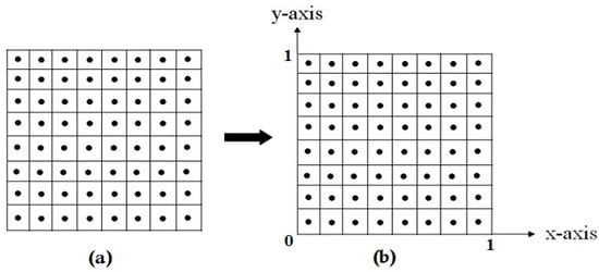
Figure 1.
(a) Discrete input image; (b) Discrete shifted Gegenbauer function.
With
The mathematical symbols, and denote the normalization constant and the fractional weight function, respectively.
2.2. 2D Shifted Fractional-Order Gegenbauer Moments
The shifted FrGMs of the order of a 2D image, of size are defined as follows:
where and are the indices of non-negative integers.
The 2D image function in is reconstructed using FrGMs as follows:
with high Max values, the reconstructed and original images, and , respectively, are nearly identical.
3. Proposed 3D FrGMs
This section introduces the proposed 3D FrGMs and the accurate and fast computation processes they use.
3.1. Definition of 3D FrGMs
For a 3D digital image with size , the 3D FrGMs of the order with are defined continuously on the cube in terms of the fractional-order Gegenbauer functions as follows:
where and .
Using the orthogonality of the fractional-order Gegenbauer functions, the 3D image function can be expressed in terms of the fractional-order shifted Gegenbauer functions on the cube :
The 3D image function in Equation (9) is approximately represented as follows:
For the intensity function of digital image f (, , ) of size , Equation (8) can be approximated as follows:
where the points (, , ) are defined as
With , and , , & .
3.2. Accurate Computation of 3D FrGMs
The approximation of the triple integration in Equation (8) resulted in numerical errors. The numerical errors grew in proportion to the order of the moments. As a result, numerical instabilities can occur when the orders reach a cretin value. Moreover, these moments are inaccurate and very time consuming. This section presents an accurate and fast method for computing 3D FrGMs. In this method, the 3D FrGMs are computed using an accurate integration method, the Gaussian quadrature method [54]. The 3D FrGMs in Equation (8) can be represented as follows:
where
Equation (14) can be expressed separately as follows:
where
For simplicity,
Using Equations (19)–(21) in Equations (16)–(18) yields the following:
where , , and .
The exact evaluation of and is impossible. As a result, an accurate Gaussian numerical integration approach is used to evaluate the kenels , and , expressed as follows:
where c, , , and denote the numerical integration order, sampling points, weights, and locations of these points, respectively.
Implementing Equation (25) into Equation (22) yields the following:
Similarly:
The Gamma and factorial functions require computationally expensive processes in Equation (15). Recurrence relations can be used to avoid these time-consuming processes. Equation (5) defines a normalization constant computed recursively as follows:
To recursively compute and , we use the recurrence relation in Equation (3) in Equations (26)–(28). Significant time savings can be achieved when Equation (15) is expressed in an inseparable form as follows:
where
And
4. Experimental Results
This section presents the experimental results for evaluating the performance and effectiveness of the proposed 3D FrGMs in the reconstruction, invariability property, noise resistance, and computation time. This section is organized into four subsections. In the first subsection, we test the performance of the 3D FrGMs to reconstruct 3D images and compare them with existing methods [31,32,43,49,50]. The invariability property of the 3D FrGMs is presented in the second subsection and compared with existing methods [31,32,43,49,50]. The noise resistance of the proposed 3D FrGMs is presented in the third subsection and compared with [26,27,38,43,44]. The last subsection compares the computation time of the proposed 3D FrGMs with the existing methods [31,32,43,49,50].
4.1. 3D Image Reconstruction
An important process in several image processing applications is 3D image/object reconstruction using FrGMs. This process is commonly used to assess the numerical stability and accuracy of OMs. A well-known quantitative metric called normalized image reconstruction error (NIRE) is used for measuring the reconstruction error as a function of the original image and the reconstructed one . The NIRE for a 3D image/object is expressed as follows:
where and represent the intensity function of the original 3D image and the intensity function of the reconstructed 3D image, respectively.
Lower NIRE values ensure accuracy, while NIRE values equal to 0 are ideal. However, these values are impossible because the reconstructed 3D image is not completely identical to the original one. Practically, with a minimum NIRE value, 3D images can be successfully and accurately reconstructed using OMs, while in practice, accurate methods approach zero. Numerical stability implies that the moments’ orders increase, while the NIRE values decrease.
To reconstruct the 3D images, we use different order moments from low to high to address the stability and accuracy of the proposed FrGMs and the compared methods. In the case of low order, all methods are used to reconstruct the 3D image, but the reconstructed image is initially not close to the original one. Therefore, a high order is gradually used to improve the quality reconstruction of 3D images, especially in accurate methods.
In the following experiment, we select “ants” as a 3D image of size 128 × 128 × 128. Voxels form the well-known Princeton Shape Benchmark (PSB) [55], as shown in Figure 2.
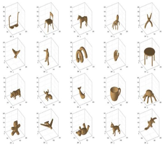
Figure 2.
Samples of 3D images from the PSB.
Another criterion that can be used for calculating the reconstruction error is the peak signal-to-noise ratio (PSNR). For good results, the PSNR must increase with increasing moment order.
where and represent the intensity function of the original 3D image and the intensity function of the reconstructed 3D image, respectively.
The new moments with fractional order (FrGMs) and the existing methods (FrOFMMs [31], FrCMs [32], FrZMs [43], FrGLMs [49], and FrOLMs [50] were used in reconstructing the 3D image “ants” with the following moment order: . For a fair comparison, the fractional parameter, α = 1.2, was used as in [50]. Moreover, we used the same object test as in [50]. Figure 3 depicts the computed values of the NIRE for the reconstructed 3D image “ants”, with the following selected moment order: .
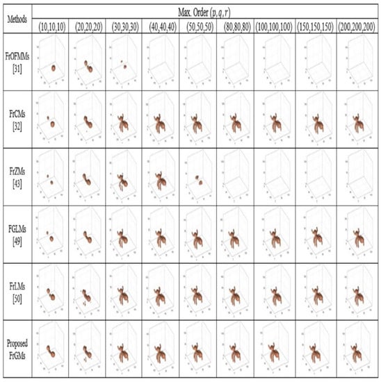
Figure 3.
The reconstructed 3D image “ant” uses the proposed FrGMs and existing methods [31,32,43,49,50].
Figure 3 and Figure 4 demonstrate how the FrOFMMs [31] and FrZMs [43] fail to reconstruct the 3D image “ant” with high quality. Figure 4 shows the reconstructed images with various 3D OMs in fractional order.

Figure 4.
The FrGMs’ NIRE values and the compared methods [31,32,43,49,50].
At higher orders, the proposed FrGMs outperformed the FrOFMMs [31] and FrZMs [43] in terms of image reconstruction visual effect while show similar ability to reconstruct 3D image with the recent orthogonal moments with fractional-order [32,49,50], FrCMs [32], FrGLMs [49] and FrOLMs [50]. Moreover, the proposed FrGMs moments best resemble the original 3D image, increasing moment order. The obtained results prove the proposed method’s stability and accuracy.
At higher orders, the proposed FrGMs outperformed the FrOFMMs [31] and FrZMs [43] in terms of the visual effect in image reconstruction while showing a similar ability to reconstruct a 3D image with the recent fractional-order OMs [32,49,50], FrCMs [32], FrGLMs [49], and FrOLMs [50]. We reconstructed the 3D images at higher orders (200, 200, and 200) for the proposed method and the existing methods [31,32,43,49,50]. We visually observed that the proposed and the existing methods in [32,49,50] are very close at higher orders, as these methods used an accurate computation technique to compute the fractional 3D moments. Conversely, the FrOFMMs [31] and FrZMs [43] had the worst performance in reconstructing the 3D images, with the order of >20 and >40, respectively, because the fractional orthogonal polynomial used in the computation of FrOFMMs and FrZMs contained factorial and power terms. These factorial and power calculations cause numerical instabilities in the procedure, and it takes an incredible amount of time to compute FrOFMMs and FrZMs, especially when the moment’s order is high. These errors affect their reconstruction (i.e., the NIRE value is divergent). Moreover, the computation of FrOFMMs and FrZMs is based on conventional direct computation, which produces two types of errors, namely geometrical and numerical. The proposed FrGMs best resemble the original 3D image, increasing the moment order. The proposed method is slightly better than those proposed in [32,49,50]. The obtained results prove the proposed method’s stability and accuracy.
4.2. Invariability
Geometric transformations—RST—are important properties for pattern recognition and computer vision applications. To test the ability invariants of the 3D moment in var-ious image transformations, the invariance to geometric transformations is quantitatively evaluated as follows:
where denotes the independent moments’ total number and and refer to the amplitude values of the used moments for the original and transformed 3D object/image, respectively. A small mean square error leads to good invariance. In this experiment, the “cups” test image, which has a size of 128 × 128 × 128 voxels (Figure 2), was chosen from the PSB database [55] to assess the proposed FrGMs’ RST invariance.
To assess the proposed FrGMs’ rotation invariance, we rotate the test image at rotation angles of 0°, 10°, 20°, …, 90°. As the invariability test is commonly used in pattern recognition applications and in watermarking the moment order in a low order, we use the moment order that is equal to 20 and calculate the proposed FrGMs, FrOFMMs [31], FrCMs [32], FrZMs [43], FrGLMs [49], and FrOLMs [50] for the transformed and original images. The results of the MSE are plotted and depicted in Figure 5.
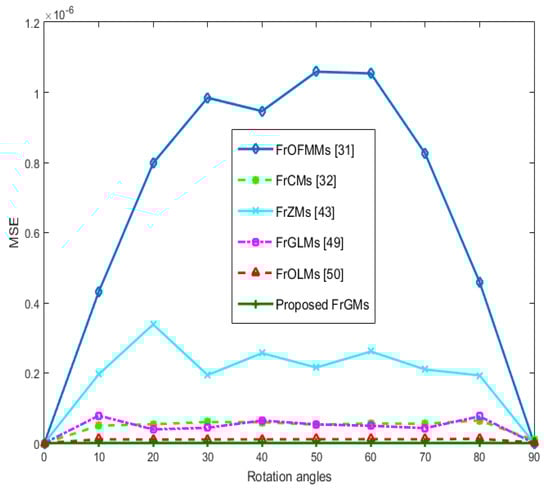
Figure 5.
Rotation MSE values using FrGMs and existing methods [31,32,43,49,50].
As shown in Figure 5, the existing methods—FrOFMMs [31], FrCMs [32], FrZMs [43], FrGLMs [49], and FrOLMs [50]—have different values of MSE greater than the corresponding values of the proposed FrGMs. The obtained results ensure that the proposed FrGMs have the lowest MSE values and achieve the best rotation invariance.
To assess the proposed FrGMs’ scaling invariance, we scale the test image using different factors, such as 0.25, 0.5, 0.75, …, and 2.0. We use a moment order that is equal to 20 and calculate the proposed FrGMs, FrOFMMs [31], FrCMs [32], FrZMs [43], FrGLMs [49], and FrOLMs [50] for the input and scaled tests for 3D object/images. The computed values using FrOFMMs [31] and FrZMs [43] give extremely poor performance. Figure 6 shows the computed MSE values for the scaled images. The obtained results ensure that the proposed FrGMs have the lowest MSE values and achieve the best scaling invariance.
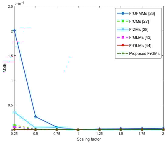
Figure 6.
Scaling values of the MSE of FrGMs and the existing methods [26,27,38,43,44].
Finally, to assess the proposed FrGMs’ translation invariance, the test image “cups” is translated at various values from (−10, −10, −10) to (10, 10, 10), with steps (2, 2, 2). We use a moment order equal to 20 and calculate the proposed FrGMs, FrOFMMs [26], FrCMs [31], FrZMs [43], FrGLMs [49], and FrOLMs [50] for the input and translated test 3D object/images. The computed values using FrOFMMs [31] and FrZMs [43] give extremely poor performance. Figure 7 shows the computed MSE values for the translated images. Again, the obtained results ensure that the proposed FrGMs have the lowest MSE values and achieve the best translation invariance. These experiments demonstrate that the FrGMs are superior to the existing methods [31,32,43,49,50], proving highly accurate RST geometric transformation invariances.
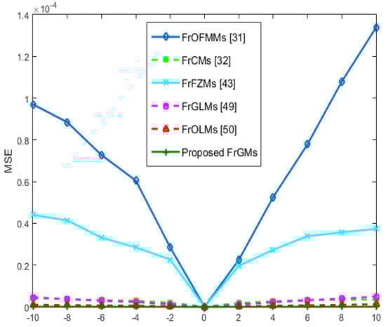
Figure 7.
The translated MSE values of FrGMs and the existing methods [31,32,43,49,50].
4.3. Noise Invariance
We performed three experiments to assess the resistance ability of FrGMs to different kinds of noises: speckles, white Gaussian, and “salt and pepper.” First, we contaminate the image “cups” [54] using various densities of “salt and pepper” noise at 0%, 0.25%, ………, and 5%. Second, we distort the image “cups” using Gaussian noise with zero mean and standard deviation values of 0, 0.05, …, and 0.5. Finally, we contaminate the image “cups” using speckle noise at 0, 0.05, …, and 1. Figure 8 shows the noisy images. We compute MSE values for the noisy image “cups” using FrGMs, FrOFMMs [31], FrCMs [32], FrZMs [43], FrGLMs [49], and FrOLMs [50]. Figure 9a–c depicts the results of the MSE values for “salt and peppers,” white Gaussian, and speckle noise, respectively. These experiments ensure the superiority of FrGMs to existing methods [31,32,43,49,50], proving that the proposed FrGMs have high resistance against different kinds of noise.
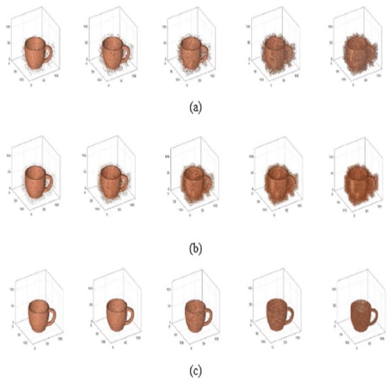
Figure 8.
Noisy 3D image: (a) “Salt and pepper“, (b) Gaussian, (c) Speckle.
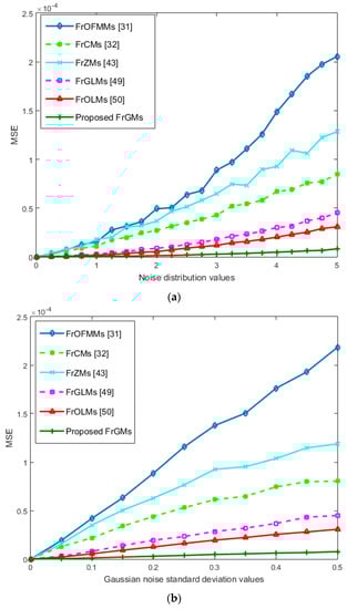
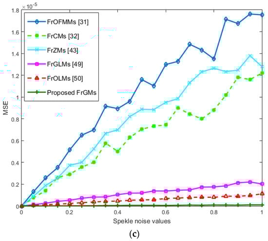
Figure 9.
MSE values of the noisy 3D image of “cups” [55] for the proposed FrGMs and the existing methods [31,32,43,49,50]: (a) “Salt and peppers”, (b) White Gaussian, (c) Speckle.
4.4. Computational Time
Efficient computation of the descriptors of the 3D image is essential in different applications. An obvious metric, execution time, evaluates any computational algorithm’s efficiency. In this subsection, the main objective is evaluating the speed of computation of the proposed FrGMs, compared with FrOFMMs [31], FrCMs [32], FrZMs [43], FrGLMs [49] and FrOLMs [50]. The well-known PSB [54] with two different sizes, 128 × 128 × 128 and 256 × 256 × 256 voxels, respectively, are utilized in the conducted experiments where the proposed FrGMs and the fractional-order OMs [31,32,43,49,50] are computed with specific orders from (0,0,0) to (16,16,16). We repeat the computing process of proposed FrGMs and the OMs of fractional orders [31,32,43,49,50] 10 times. Then, the average elapsed CPU times are plotted and displayed in Figure 10. Figure 10 clearly demonstrate the proposed FrSGMs are much faster than the fractional-order OMs [31,32,43,49,50].
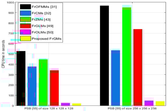
Figure 10.
The average CPU times of the proposed FrGMs and the existing methods [31,32,43,49,50].
To support the above discussion, we compute the overall computational complexity of the proposed FrGMs. We consider the different papermakers in the computations as the moments’ order , the size of the input 3D image, and the radial and angular kernels. For a 3D digital image with size , the overall computational complexity of the FrGMs is O(FrGMs) = O (calculation of the radial kernel in the x direction) + O (calculation of the radial kernel in the y direction) + O (calculation of the radial kernel in the z direction) + O (the product of radial kernels and the 3D image function in Cartesian). Therefore, . If we take , the computation complexity is , and the proposed exhibit is .
Based on all the numerical experiments, we can conclude that the proposed algorithm achieved the best performance in reconstructing 3D images with the lowest NIRE values and computation time compared with the existing algorithms. The proposed algorithm has advantages over existing algorithms [31,32,43,49,50] due to the new descriptor, which has remarkable characteristics that represent the accurate features of 3D images and the fast, effective, and accurate computation method of FrGMs.
5. Conclusions
Fractional-order OMs have remarkable characteristics that represent 2D and 3D im-ages. Most existing studies have focused on 2D images. In our lives, many applications are based on the representation of 3D images, and these applications require an accurate and fast method to extract the features of 3D images. Thus, the main objective of this paper was to present novel 3D-object/image-descriptor-shifted FrGMs. These new descriptors were defined and computed in the Cartesian domain on the cube. Computing these new descriptors did not require image mapping, which avoided interpolation and geometric errors produced by computing the fractional-order OMs. A very fast, accurate computational method was used to compute the new descriptors, avoiding integration error and removing high-order numerical instability. Several numerical experiments were performed to investigate the efficacy of the proposed shifted FrGMs in 3D image reconstruction capabilities, invariance to RST, noise resistance, and computation time. In general, the proposed FrGMs perform better than the compared methods. In the future, we can extend this work to design a suitable algorithm to deal with biological 3D problems, such as protein docking. Using the fast Fourier transform, we can design a memory-efficient algorithm for computing FrGMs. We can also focus on real-life applications, such as 3D medical images, 3D facial recognition, 3D object retrieval, and 3D stereoscopic images. In addition, we will accelerate the computation of 3D FrGMs and its in-variability to deal with many 3D images in different applications.
Author Contributions
Methodology, M.M.D.; Software, D.S.K. and M.M.D.; Resources, A.A.A.; Writing—original draft, M.M.D.; Writing—review & editing, D.S.K., A.A.A. and K.M.H.; Supervision, K.M.H.; Funding acquisition, D.S.K. and A.A.A. All authors have read and agreed to the published version of the manuscript.
Funding
This research was funded by Princess Nourah bint Abdulrahman University Researchers Supporting Project number (PNURSP2022R308), Princess Nourah bint Abdulrahman University, Riyadh, Saudi Arabia.
Institutional Review Board Statement
Not applicable.
Informed Consent Statement
Not applicable.
Data Availability Statement
The data used to support the findings of this study are available from the corresponding author upon request.
Acknowledgments
Princess Nourah bint Abdulrahman University Researchers Supporting Project number (PNURSP2022R308), Princess Nourah bint Abdulrahman University, Riyadh, Saudi Arabia.
Conflicts of Interest
The authors declare no conflict of interest.
References
- Wang, C.; Wang, X.; Xia, Z.; Ma, B.; Shi, Y.Q. Image description with polar harmonic Fourier moments. IEEE Trans. Circuits Syst. Video Technol. 2019, 30, 4440–4452. [Google Scholar] [CrossRef]
- Hosny, K.M.; Darwish, M.M.; Aboelenen, T. Novel fractional-order polar harmonic transforms for gray-scale and color image analysis. J. Frankl. Inst. 2020, 357, 2533–2560. [Google Scholar] [CrossRef]
- Xia, Z.; Wang, X.; Zhou, W.; Li, R.; Wang, C.; Zhang, C. Color medical image lossless watermarking using chaotic system and accurate quaternion polar harmonic transforms. Signal Process 2019, 157, 108–118. [Google Scholar] [CrossRef]
- Teague, M.R. Image analysis via the general theory of moments. J. Opt. Soc. Am. 1980, 70, 920–930. [Google Scholar] [CrossRef]
- Papakostas, G. Over 50 Years of Image Moments and Moment Invariants. Moments Moment Invariants-Theory Appl. 2014, 1, 3–32. [Google Scholar]
- Flusser, J.; Suk, T.; Zitova, B. 2D and 3D Image Analysis by Moments; John Wiley & Sons: Hoboken, NJ, USA, 2016; ISBN 9781119039372. [Google Scholar]
- Yue, C. A study on the correlation between pre-translation preparation with 3D virtual reality technology and the cognitive load of consecutive interpreting. Foreign Lang. Teach. 2021, 42, 93–97. [Google Scholar]
- Qi, S.; Ning, X.; Yang, G.; Zhang, L.; Long, P.; Cai, W.; Li, W. Review of Multi-view 3D Object Recognition Methods Based on Deep Learning. Displays 2021, 69, 102053. [Google Scholar] [CrossRef]
- Angelopoulou, A.; Psarrou, A.; Garcia-Rodriguez, J.; Orts-Escolano, S.; Azorin-Lopez, J.; Revett, K. 3D reconstruction of medical images from slices automatically landmarked with growing neural models. Neurocomputing 2015, 150, 16–25. [Google Scholar] [CrossRef]
- Manor, A.; Fischer, A. Reverse Engineering of 3D Models Based on Image Processing and 3D Scanning Techniques. In International Workshop on Geometric Modelling; Kimura, F., Ed.; Springer: Boston, MA, USA, 2001. [Google Scholar] [CrossRef][Green Version]
- Lohmann, G. Volumetric Image Analysis; John Wiley & Sons: Hoboken, NJ, USA, 1998; ISBN 9780471967859. [Google Scholar]
- Benouini, R.; Batioua, I.; Zenkouar, K.; Najah, S.; Qjidaa, H. Efficient 3D object classification by using direct Krawtchouk moment invariants. Multimed. Tools Appl. 2018, 77, 27517–27542. [Google Scholar] [CrossRef]
- Kumar, B. Hyperspectral image classification using three-dimensional geometric moments. IET Image Process 2020, 14, 2175–2186. [Google Scholar] [CrossRef]
- Karmouni, H.; Jahid, T.; Sayyouri, M.; El Alami, R.; Qjidaa, H. Fast 3D image reconstruction by cuboids and 3D Charlier’s moments. J. Real-Time Image Process 2020, 17, 949–965. [Google Scholar] [CrossRef]
- Yang, F.; Ding, M.; Zhang, X. Non-rigid multi-modal 3D medical image registration based on foveated modality independent neighborhood descriptor. Sensors 2019, 19, 4675. [Google Scholar] [CrossRef] [PubMed]
- Karmouni, H.; Yamni, M.; Daoui, A.; Sayyouri, M.; Qjidaa, H. Fast computation of 3D Meixner’s invariant moments using 3D image cuboid representation for 3D image classification. Multimed. Tools Appl. 2020, 79, 29121–29144. [Google Scholar] [CrossRef]
- Tahiri, M.A.; Karmouni, H.; Sayyouri, M.; Qjidaa, H. 2D and 3D image localization, compression, and reconstruction using new hybrid moments. Multidimens. Syst. Signal Process 2022, 33, 1–38. [Google Scholar] [CrossRef]
- Sayyouri, M.; Karmouni, H.; Hmimid, A.; Azzayani, A.; Qjidaa, H. A fast and accurate computation of 2D and 3D generalized Laguerre moments for images analysis. Multimed. Tools Appl. 2021, 80, 7887–7910. [Google Scholar] [CrossRef]
- Hosny, K.M. Fast and low-complexity method for exact computation of 3D Legendre moments. Pattern Recognit. Lett. 2011, 32, 1305–1314. [Google Scholar] [CrossRef]
- Karmouni, H.; Yamni, M.; El Ogri, O.; Daoui, A.; Sayyouri, M.; Qjidaa, H.; Tahiri, A.; Maaroufi, M.; Alami, B. Fast computation of 3D discrete invariant moments based on 3D cuboid for 3D image classification. Circuits Syst. Signal Process 2021, 40, 3782–3812. [Google Scholar] [CrossRef]
- Sit, A.; Shin, W.H.; Kihara, D. Three-dimensional Krawtchouk descriptors for protein local surface shape comparison. Pattern Recognit. 2019, 93, 534–545. [Google Scholar] [CrossRef]
- Jahid, T.; Karmouni, H.; Sayyouri, M.; Hmimid, A.; Qjidaa, H. Fast algorithm of 3D discrete image orthogonal moments computation based on 3D cuboid. J. Math. Imaging Vis. 2019, 61, 534–554. [Google Scholar] [CrossRef]
- Yamni, M.; Daoui, A.; Karmouni, H.; Sayyouri, M.; Qjidaa, H. Accurate 2D, and 3D images classification using translation and scale invariants of Meixner moments. Multimed. Tools Appl. 2021, 80, 26683–26712. [Google Scholar] [CrossRef]
- Rivera-Lopez, J.S.; Camacho-Bello, C.; Vargas-Vargas, H.; Escamilla-Noriega, A. Fast computation of 3D Tchebichef moments for higher orders. J. Real-Time Image Process. 2022, 19, 15–27. [Google Scholar] [CrossRef]
- Lakhili, Z.; El Alami, A.; Mesbah, A.; Berrahou, A.; Qjidaa, H. Robust classification of 3D objects using discrete orthogonal moments and deep neural networks. Multimed Tools Appl. 2020, 79, 18883–18907. [Google Scholar] [CrossRef]
- Yamni, M.; Daoui, A.; Karmouni, H.; Sayyouri, M.; Qjidaa, H.; Maaroufi, M.; Alami, B. Fast and Accurate Computation of 3D Charlier Moment Invariants for 3D Image Classification. Circuits Syst. Signal Process 2021, 40, 6193–6223. [Google Scholar] [CrossRef]
- Batioua, I.; Benouini, R.; Zenkouar, K.; Zahi, A. 3D image analysis by separable discrete orthogonal moments based on Krawtchouk and Tchebichef polynomials. Pattern Recognit. 2017, 71, 264–277 4. [Google Scholar] [CrossRef]
- Lakhili, Z.; El Alami, A.; Mesbah, A.; Berrahou, A.; Qjidaa, H. Rigid and non-rigid 3D shape classification based on 3D Hahn moments neural networks model. Multimed. Tools Appl. 2022, 1–24. [Google Scholar] [CrossRef]
- Xiao, B.; Li, L.; Li, Y.; Li, W.; Wang, G. Image analysis by fractional-order orthogonal moments. Inf. Sci. 2017, 382, 135–149. [Google Scholar] [CrossRef]
- Hosny, K.M.; Darwish, M.M.; Aboelenen, T. New Fractional-order Legendre-Fourier moments for pattern recognition applications. Pattern Recognit. 2020, 103, 1–19. [Google Scholar] [CrossRef]
- Zhang, H.; Li, Z.; Liu, Y. Fractional orthogonal Fourier-Mellin moments for pattern recognition. In Chinese Conference on Pattern Recognition; Springer: Singapore, 2016; pp. 766–778. [Google Scholar]
- Benouini, R.; Batioua, I.; Zenkouar, K.; Zahi, A.; Najah, S.; Qjidaa, H. Fractional-order orthogonal Chebyshev moments and moment invariants for image representation and pattern recognition. Pattern Recognit. 2019, 86, 332–343. [Google Scholar] [CrossRef]
- Wang, C.; Gao, H.; Yang, M.; Li, J.; Ma, B.; Hao, Q. Invariant image representation using novel fractional-order polar harmonic Fourier moments. Sensors 2021, 21, 1544. [Google Scholar] [CrossRef]
- Tao, F.; Qian, W. Image hash authentication algorithm for orthogonal moments of fractional-order chaotic scrambling coupling hyper-complex number. Measurement 2019, 134, 866–873. [Google Scholar] [CrossRef]
- Yang, B.; Shi, X.; Chen, X. Image Analysis by Fractional-Order Gaussian-Hermite Moments. IEEE Trans. Image Process. 2022, 31, 2488–2502. [Google Scholar] [CrossRef] [PubMed]
- Chen, B.; Yu, M.; Su, Q.; Shim, H.J.; Shi, Y.Q. Fractional quaternion Zernike moments for robust color image copy-move forgery detection. IEEE Access 2018, 6, 56637–56646. [Google Scholar] [CrossRef]
- Hosny, K.M.; Darwish, M.M.; Aboelenen, T. Novel Fractional-Order Generic Jacobi-Fourier Moments for Image Analysis. Signal Process. 2020, 172, 107545. [Google Scholar] [CrossRef]
- He, B.; Liu, J.; Yang, T.; Xiao, B.; Peng, Y. Quaternion fractional-order color orthogonal moment-based image representation and recognition. EURASIP J. Image Video Process 2021, 1, 1–35. [Google Scholar] [CrossRef]
- Daoui, A.; Yamni, M.; Karmouni, H.; Sayyouri, M.; Qjidaa, H. Biomedical signals reconstruction and zero-watermarking using separable fractional order Charlier–Krawtchouk transformation and sine cosine algorithm. Signal Process 2021, 180, 107854. [Google Scholar] [CrossRef]
- Xiao, B.; Luo, J.; Bi, X.; Li, W.; Chen, B. Fractional discrete Tchebyshev moments and their applications in image encryption and watermarking. Inf. Sci. 2020, 516, 545–559. [Google Scholar] [CrossRef]
- Hosny, K.M.; Abd Elaziz, M.; Darwish, M.M. Color face recognition using novel fractional-order multi-channel exponent moments. Neural Comput. Appl. 2021, 33, 5419–5435. [Google Scholar] [CrossRef]
- Wang, C.; Hao, Q.; Ma, B.; Wu, X.; Li, J.; Xia, Z.; Gao, H. Octonion continuous orthogonal moments and their applications in color stereoscopic image reconstruction and zero-watermarking. Eng. Appl. Artif. Intell. 2021, 106, 104450. [Google Scholar] [CrossRef]
- Kaur, P.; Pannu, H.S.; Malhi, A.K. Plant disease recognition using fractional-order Zernike moments and SVM classifier. Neural Comput. Appl. 2019, 31, 8749–8768. [Google Scholar] [CrossRef]
- Hosny, K.M.; Darwish, M.M.; Fouda, M.M. Robust color images watermarking using new fractional-order exponent moments. IEEE Access 2021, 9, 47425–47435. [Google Scholar] [CrossRef]
- Duan, C.F.; Zhou, J.; Gong, L.H.; Wu, J.Y.; Zhou, N.R. New color image encryption scheme based on multi-parameter fractional discrete Tchebyshev moments and nonlinear fractal permutation method. Opt. Lasers Eng. 2022, 150, 106881. [Google Scholar] [CrossRef]
- Wang, C.; Ma, B.; Xia, Z.; Li, J.; Li, Q.; Shi, Y.Q. Stereoscopic image description with trinion fractional-order continuous orthogonal moments. IEEE Trans. Circuits Syst. Video Technol. 2021, 32, 1998–2012. [Google Scholar] [CrossRef]
- Benouini, R.; Batioua, I.; Zenkouar, K.; Najah, S. Fractional-order generalized Laguerre moments and moment invariants for grey-scale image analysis. IET Image Process. 2021, 15, 523–541. [Google Scholar] [CrossRef]
- Daoui, A.; Yamni, M.; Karmouni, H.; Sayyouri, M.; Qjidaa, H.; Ahmad, M.; Abd El-Latif, A.A. Biomedical Multimedia encryption by fractional-order Meixner polynomials map and quaternion fractional-order Meixner moments. IEEE Access 2022, 10, 102599–102617. [Google Scholar] [CrossRef]
- El Ogri, O.; Daoui, A.; Yamni, M.; Karmouni, H.; Sayyouri, M.; Qjidaa, H. New set of fractional-order generalized Laguerre moment invariants for pattern recognition. Multimed Tools Appl. 2020, 79, 23261–23294. [Google Scholar] [CrossRef]
- El Ogri, O.; Karmouni, H.; Sayyouri, M.; Qjidaa, H. 3D image recognition using new set of fractional-order Legendre moments and deep neural networks. Signal Process. Image Commun. 2021, 98, 116410. [Google Scholar] [CrossRef]
- Hosny, K.M.; Darwish, M.M.; Eltoukhy, M.M. New fractional-order shifted Gegenbauer moments for image analysis and recognition. J. Adv. Res. 2020, 25, 57–66. [Google Scholar] [CrossRef]
- Hafez, R.M.; Youssri, Y.H. Shifted Gegenbauer–Gauss collocation method for solving fractional neutral functional-differential equations with proportional delays. Kragujev. J. Math. 2022, 46, 981–996. [Google Scholar] [CrossRef]
- Issa, K.; Yisa, B.M.; Biazar, J. Numerical solution of space fractional diffusion equation using shifted Gegenbauer polynomials. Comput. Methods Differ. Equ. 2022, 10, 431–444. [Google Scholar]
- Faires, J.D.; Burden, R.L. Numerical Methods, 3rd ed.; Brooks Cole Publication: Monterey, CA, USA, 2002. [Google Scholar]
- Shilane, P.; Min, P.; Kazhdan, M.; Funkhouser, T. The Princeton Shape Benchmark. In Proceedings Shape Modeling Applications; IEEE: New York, NY, USA, 2004; pp. 167–178. [Google Scholar]
Publisher’s Note: MDPI stays neutral with regard to jurisdictional claims in published maps and institutional affiliations. |
© 2022 by the authors. Licensee MDPI, Basel, Switzerland. This article is an open access article distributed under the terms and conditions of the Creative Commons Attribution (CC BY) license (https://creativecommons.org/licenses/by/4.0/).