Article

Global Stability of Delayed SARS-CoV-2 and HTLV-I Coinfection Models within a Host

Department of Mathematics, Faculty of Science, King Abdulaziz University, P.O. Box 80203, Jeddah 21589, Saudi Arabia
*
Author to whom correspondence should be addressed.
Mathematics 2022, 10(24), 4756; https://doi.org/10.3390/math10244756
Submission received: 17 November 2022 / Revised: 1 December 2022 / Accepted: 8 December 2022 / Published: 14 December 2022

Abstract

:
The aim of the present paper is to formulate two new mathematical models to describe the co-dynamics of severe acute respiratory syndrome coronavirus 2 (SARS-CoV-2) and human T-cell lymphotropic virus type-I (HTLV-I) in a host. The models characterizes the interplaying between seven compartments, uninfected ECs, latently SARS-CoV-2-infected ECs, actively SARS-CoV-2-infected ECs, free SARS-CoV-2 particles, uninfected CD4 + T cells, latently HTLV-I-infected CD4 + T cells and actively HTLV-I-infected CD4 + T cells. The models incorporate five intracellular time delays: (i) two delays in the formation of latently SARS-CoV-2-infected ECs and latently HTLV-I-infected CD4 + T cells, (ii) two delays in the reactivation of latently SARS-CoV-2-infected ECs and latently HTLV-I-infected CD4 + T cells, and (iii) maturation delay of new SARS-CoV-2 virions. We consider discrete-time delays and distributed-time delays in the first and second models, respectively. We first investigate the properties of the model’s solutions, then we calculate all equilibria and study their global stability. The global asymptotic stability is examined by constructing Lyapunov functionals. The analytical findings are supported via numerical simulation. The impact of time delays on the coinfection progression is discussed. We found that, increasing time delays values can have an antiviral treatment-like impact. Our developed coinfection model can contribute to understand the SARS-CoV-2 and HTLV-I co-dynamics and help to select suitable treatment strategies for COVID-19 patients with HTLV-I.
MSC:
34D20; 34D23; 37N25; 92B05

1. Introduction

At the end of 2019, the world witnessed the emergence of a new infectious disease in Wuhan, China, which was called coronavirus disease 2019 (COVID-19). This disease is caused by severe acute respiratory syndrome coronavirus 2 (SARS-CoV-2). Within a few months, SARS-CoV-2 infection spread rapidly in most countries of the world and infected many people. According to the update provided by the World Health Organization (WHO) on 23 October 2022 [1], over 624 million confirmed cases and over 6.5 million deaths have been reported globally. SARS-CoV-2 is transmitted to people when they are exposed to respiratory fluids carrying infectious viral particles. The implementation of preventive measures such as hand washing, using of face masks, physical and social distancing, disinfection of surfaces and getting COVID-19 vaccine can reduce the SARS-CoV-2 transmission. WHO approved eleven vaccines for COVID-19 for emergency use including Novavax, CanSino, Bharat Biotech, Pfizer/BioNTech, Moderna, Serum Institute of India (Novavax formulation), Janssen (Johnson & Johnson), Oxford/AstraZeneca, Serum Institute of India (Oxford/AstraZeneca formulation), Sinopharm, and Sinovac [2].
SARS-CoV-2 is a single-stranded positive-sense RNA virus and infects the ECs of the respiratory tracts. The virus has clinical manifestations including dyspnea, cough, fever, headache, rhinitis, myalgia and sore throat. SARS-CoV-2 can lead to acute respiratory distress syndrome (ARDS), which has high mortality rates, particularly in patients with immunosenescence [3] susceptibility to viral infections [4]. It was reported in [5] that, 94.2% of patients with COVID-19 were also coinfected with several other microorganisms, such as fungi, bacteria and viruses. Important viral copathogens include the respiratory syncytial virus, rhinovirus/enterovirus, influenza A and B viruses (IAV and IBV), metapneumovirus, parainfluenza virus, human immunodeficiency virus (HIV), cytomegalovirus (CMV), dengue virus (DENV), hepatitis B virus (HBV) and Epstein Barr virus (EBV) (see the review paper [6]).
Human T-cell lymphotropic virus type-I (HTLV-I) is a single-stranded RNA virus which infects the essential human system immune cells, CD4 + T cells. Therefore, HTLV-I can cause immune dysfunction even in asymptomatic carriers [3]. HTLV-I can leads to two diseases, adult T-cell leukemia (ATL) and HTLV-I-associated myelopathy/tropical spastic paraparesis (HAM/TSP) [7]. Although HTLV-I can cause fatal diseases (ATL and HAM/TSP), most of infected persons remain asymptomatic throughout their lives [3]. An estimation by WHO told that about 5 to 10 million individuals are infected with HTLV-I worldwide [8]. The primary way for HTLV-I transmission is through bodily fluids including: semen, blood and breast milk [9]. The spread of this viral infection that causes significant morbidity and mortality in some countries of the world has increased the interest and awareness of medical and biological scientists.
In [3,10], two cases of COVID-19 patients with HTLV-I infection were reported. These reports highlighted the need for the accumulation of similar cases to illustrate the risk factors for severe illness, the best-in-class antiviral agent, how to manage and prevent secondary infection, and the optimal treatment strategy for patients with SARS-CoV-2 and HTLV-I coinfection. Sajjadi et al. [11] presented a review on the pathogenesis of both SARS-CoV-2 and HTLV-I infections and discussed their similarities in triggering immune responses.

Mathematical Models of Within-Host HTLV-I and SARS-CoV-2 Mono-Infections

During the past decade, mathematical models which describe the within-host dynamics of human viruses have demonstrated their ability to provide useful insight to gain a further understanding the dynamics and mechanisms of the viruses. These models may assist in the development of viral therapies and vaccines as well as the selection of appropriate therapeutic and vaccine strategies. Further, these models are helpful in determine the sufficient number of factors to analyze the experimental results and explain the biological phenomena [12]. Furthermore, mathematical models have been a key in studying viral-viral coinfections and can be particularly useful in examining the interplay between respiratory viruses and chronic viruses.
Hernandez-Vargas and Velasco-Hernandez [13] formulated the basic target cell-limited model for SARS-CoV-2 dynamics within a host. The model contained three compartments, uninfected ECs (X), active SARS-CoV-2-infected ECs (Y) and free SARS-CoV-2 particles (V). The model was formulated as a system of ODEs:
X ˙ ( t ) = ρ V ( t ) X ( t ) SARS - CoV - 2 infectious transmission ,
Y ˙ ( t ) = ρ V ( t ) X ( t ) SARS - CoV - 2 infectious transmission ξ Y Y ( t ) death ,
V ˙ ( t ) = η Y ( t ) generation of SARS - CoV - 2 ξ V V ( t ) death .
In the same paper [13], this model was extended to include the eclipse (latent) phase. The eclipse phase is defined as the period of time that elapses between the entry of the virus into the uninfected epithelial cell and the release of virions from that infected cell [14]. There are two methods to include the latent phase in the viral infection models. The first method is to comprise the eclipse phase by introducing it as a time delay in the model [15]. This can be conducted by reformulating Equation (2) as [15]:
Y ˙ ( t ) = ρ V ( t τ ) X ( t τ ) ξ Y Y ( t ) ,
where τ is the delay between viral entry into an epithelial cell and the start of production IAV virions. The second method is to define two separate populations of SARS-CoV-2-infected ECs: one population is the latently SARS-CoV-2-infected cells (N) which contains the SARS-CoV-2 virions but not yet producing it; the second population is the actively SARS-CoV-2-infected cells (Y) which produce the SARS-CoV-2 [16]. SARS-CoV-2 infection model with latent infected cells was formulated as [13]:
X ˙ ( t ) = ρ V ( t ) X ( t ) SARS - CoV - 2 infectious transmission , N ˙ ( t ) = ρ V ( t ) X ( t ) SARS - CoV - 2 infectious transmission κ N ( t ) latent activation , Y ˙ ( t ) = κ N ( t ) latent activation ξ Y Y ( t ) death , V ˙ ( t ) = η Y ( t ) generation of SARS - CoV - 2 ξ V V ( t ) death .
Li et al. [17] have considered a SARS-CoV-2 infection model with regeneration and death for the uninfected ECs as:
X ˙ = δ ξ X X ρ V X ,
where δ and ξ X X are the regeneration and death rates of uninfected ECs, respectively. Models presented in [13,17] were extended and modified by including (i) the effect of immune response [18,19,20,21,22,23], (ii) the influence of different drug therapies [24,25], and (iii) the impact of time delay [26].
In very recent works, mathematical models have been formulated to describe the coinfection of COVID-19 with other diseases in epidemiology such as: COVID-19/Dengue [27], COVID-19/Influenza [28], COVID-19/HIV [29], COVID-19/ZIKV [30], COVID-19/Dengue/ HIV [31], COVID-19/Tuberculosis [32], COVID-19/Bacterial [33]. However, modeling of within-host dynamics of SARS-CoV-2 with other pathogens coinfection has been investigated in a few papers: SARS-CoV-2/Bacteria [34], SARS-CoV-2/HIV [35], SARS-CoV-2/malaria [36] and SARS-CoV-2/Influenza A virus [37].
Stability analysis of viral infection models can help researchers to (i) expect the qualitative features of the model for a given set of values of the model’s parameters, (ii) establish the conditions that ensure the persistence or deletion of this infection, and (iii) determine under what conditions the immune system is stimulated against the infection. Stability of time-delay systems has received great interest in different fields (see e.g., [38,39,40,41]). Stability analysis for models describing the within-host dynamics of SARS-CoV-2 infection was studied in [21,22,23,35,37,42]. Hattaf and Yousfi [21] studied a within-host SARS-CoV-2 infection model with cell-to-cell transmission and Cytotoxic T lymphocyte (CTL) immune response. The model included both lytic and nonlytic immune responses. Lyapunov method was used to prove the global stability of the three equilibria of the model. A SARS-CoV-2 infection model with both CTL and antibody immunities was developed and analyzed in [23]. Mathematical analysis of the model presented in [17] was studied in [42]. Both local and global stability analysis of the model’s equilibria were established. Almocera et al. [22] studied the stability of the two-dimensional SARS-CoV-2 dynamics model with immune response presented in [13]. Elaiw et al. [26] studied the global stability of a delayed SARS-CoV-2 dynamics model with logistic growth of the uninfected ECs and antibody immunity. In very recent works, Lyapunov method was used to establish the global stability of coinfection models including, SARS-CoV-2/HIV-1 [35], SARS-CoV-2/Influenza A virus [37] and SARS-CoV-2/malaria [36].
Modeling and analysis of HTLV-I mono-infection have attracted the interest of several mathematician. HTLV-I mono-infection model which describes the interaction of three compartments, healthy (or uninfected) CD4 + T cells (U), latently HTLV-I-infected cells (L) and actively HTLV-I-infected cells (A), is given by [43]:
U ˙ = γ CD 4 + T cells production ξ U U death π A U HTLV - I infectious transmission ,
L ˙ = π A U HTLV - I infectious transmission α L latent activation ξ L L death ,
A ˙ = α L latent activation ξ A * A death .
In [44], model (4)–(6) was extended by incorporating a time delay τ which accounts the time between initial infection of an uninfected target cells to become latently infected cells. Equation (5) was replaced by
L ˙ t = π A t τ U t τ α + ξ L L t .
Different biological factors were considered in HTLV-I infection models including (i) Cytotoxic T-Lymphocytes (CTLs) immunity [7,45,46,47,48], (ii) mitotic transmission of actively infected cells [49,50,51,52,53], (iii) intracellular time delay [44,47,48]) or immune response delay [45,46,54], and (iv) reaction and diffusion [55]. HTLV-I has quite similar ways of transmissions as HIV-1. Therefore, we formulated and analyzed some HIV-1/HTLV-I coinfection models [56].
To the best of our knowledge, mathematical modeling of within-host SARS-CoV-2 and HTLV-I coinfection has not been studied before. The objective of this work is to formulate new models for within-host SARS-CoV-2-HTLV-I coinfection with discrete/distributed time delays. We study the properties of the model’s solutions, calculate all equilibrium points, investigate the global stability of equilibria and conduct some numerical simulations. Finally, we discuss the obtained results.
The SARS-CoV-2 and HTLV-I coinfection models presented in this paper can be helpful to describe the co-dynamics of several human viruses. In addition, the models may be used to predict new treatment regimens and strategies for patients who are coinfected with different viruses or multi variants of a virus [57].

2. SARS-CoV-2 and HTLV-I Coinfection Model with Discrete-Time Delays

In this section, we formulate a SARS-CoV-2 and HTLV-I coinfection dynamics model. Let us consider following hypothesis:
Hypothesis 1 (H1).
The model describes the interactions between seven compartments, uninfected ECs (X), latently SARS-CoV-2-infected cells (N), actively SARS-CoV-2-infected cells (Y), free SARS-CoV-2 particles (V), uninfected CD4 + T cells (U), latently HTLV-I-infected cells (L) and actively HTLV-I-infected cells (A).
Hypothesis 2 (H2).
The uninfected ECs and CD4 + T cells are the targets for SARS-CoV-2 and HTLV-I, respectively, [13,43].
Hypothesis 3 (H3).
The CD4 + T cells help the CTLs to kill the actively SARS-CoV-2-infected ECs at rate μ Y U and are proliferated at rate u Y U [35].
Hypothesis 4 (H4).
The actively HTLV-I-infected cells are proliferated at rate ε * A , with a part ω ε * A turn into latent, while the other part ( 1 ω ) ε * A remains active, where ω ( 0 , 1 ) [52,56].
Hypothesis 5 (H5).
There exist two time delays τ 1 and τ 4 in the formation of latently SARS-CoV-2-infected cells and latently HTLV-I-infected, respectively [26,58,59].
Hypothesis 6 (H6).
There exist two reactivation time delays τ 2 and τ 5 of the latently SARS-CoV-2-infected cells and latently HTLV-I-infected cells, respectively [26,58,59].
Hypothesis 7 (H7).
There exist a maturation time delay τ 3 of SARS-CoV-2 virions [26].
Under hypothesis H1–H7 we propose the model for SARS-CoV-2 and HTLV-I coinfection within a host as:
X ˙ ( t ) = δ ξ X X t ρ V ( t ) X t ,
N ˙ ( t ) = ρ e d 1 τ 1 V ( t τ 1 ) X t τ 1 κ + ξ N N t ,
Y ˙ ( t ) = κ e d 2 τ 2 N t τ 2 ξ Y Y t μ Y t U t ,
V ˙ ( t ) = η e d 3 τ 3 Y t τ 3 ξ V V t ,
U ˙ t = γ + u Y t U t ξ U U t π A t U t ,
L ˙ t = π e d 4 τ 4 A t τ 4 U t τ 4 + ω ε * A t α + ξ L L t ,
A ˙ t = α e d 5 τ 5 L t τ 5 + ( 1 ω ) ε * A t ξ A * A t .
The factors e d 1 τ 1 , e d 2 τ 2 , e d 3 τ 3 , e d 4 τ 4 and e d 5 τ 5 denote the probability of surviving the compartments during the time delay periods, where, d 1 , d 2 , d 3 , d 4 and d 5 are constants. Let τ * = max τ 1 , τ 2 , τ 3 , τ 4 , τ 5 and assume the initial conditions of system (7)–(13) having the following form:
X ( θ ) = ϕ 1 ( θ ) , N ( θ ) = ϕ 2 ( θ ) , Y ( θ ) = ϕ 3 ( θ ) , V ( θ ) = ϕ 4 ( θ ) , U ( θ ) = ϕ 5 ( θ ) , L ( θ ) = ϕ 6 ( θ ) , A ( θ ) = ϕ 7 ( θ ) , ϕ i ( θ ) 0 , θ τ * , 0 , i = 1 , 2 , , 7 ,
where ϕ i C and C = C τ * , 0 , R 0 is the Banach space of continuous mapping the interval τ * , 0 into R 0 with the norm ϕ i = sup τ * θ 0 ϕ i ( θ ) for ϕ i C , i = 1 , 2 , , 7 . By the fundamental theory of functional differential equations, system (7)–(13) with initial conditions (14) has a unique solution [60]. We note that, model (7)–(13) can be seen as a generalization of many models for HTLV-I and SARS-CoV-2 mono-infections presented in the literature.
All parameters of model (7)–(13) are positive. In [52,56], it was proposed that ε * < min { ξ U , ξ L , ξ A * } . Since 0 < ω < 1 and ε * < ξ A * , thus ( 1 ω ) ε * < ξ A * . Denote ξ A = ξ A * ( 1 ω ) ε * > 0 and ε = ω ε * . We have ξ A ε = ξ A * ε * > 0 . Therefore, model (7)–(13) becomes:
X ˙ ( t ) = δ ξ X X t ρ V ( t ) X t ,
N ˙ ( t ) = ρ e d 1 τ 1 V ( t τ 1 ) X t τ 1 κ + ξ N N t ,
Y ˙ ( t ) = κ e d 2 τ 2 N t τ 2 ξ Y Y t μ Y t U t ,
V ˙ ( t ) = η e d 3 τ 3 Y t τ 3 ξ V V t ,
U ˙ t = γ + u Y t U t ξ U U t π A t U t ,
L ˙ t = π e d 4 τ 4 A t τ 4 U t τ 4 + ε A t α + ξ L L t ,
A ˙ t = α e d 5 τ 5 L t τ 5 ξ A A t .
Next, we will examine the nonnegativity and boundedness of the system’s solutions.

2.1. Properties of Solutions

Lemma 1.
The solutions of model (15)–(21) with initial conditions (14) are nonnegative and ultimately bounded.
Proof. 
From Equations (15) and (19), we obtain X ˙ X = 0 = δ > 0 and U ˙ U = 0 = γ > 0 . It follows that X t > 0 and U t > 0 , for all t 0 . From Equations (16)–(18), (20) and (21) we have
N t = e κ + ξ N t ϕ 2 0 + ρ e d 1 τ 1 0 t e κ + ξ N ( t θ ) V ( θ τ 1 ) X θ τ 1 d θ 0 , Y t = e 0 t ξ Y + μ U ϰ d ϰ ϕ 3 0 + κ e d 2 τ 2 0 t e θ t ξ Y + μ U ϰ d ϰ N ( θ τ 2 ) d θ 0 , V t = e ξ V t ϕ 4 0 + η e d 3 τ 3 0 t e ξ V ( t θ ) Y θ τ 3 d θ 0 , L t = e α + ξ L t ϕ 6 0 + 0 t e α + ξ L ( t θ ) π e d 4 τ 4 A θ τ 4 U θ τ 4 + ε A θ d θ 0 , A t = e ξ A t ϕ 7 0 + α e d 5 τ 5 0 t e ξ A ( t θ ) L θ τ 5 d θ 0 ,
for all t 0 , τ * . Hence, by a recursive argument, we obtain N t , Y t , V t , L t , A t 0 for all t 0 . This guarantees that X t , N t , Y t , V t , U t , L t , A t R 0 7 for all t 0 if X 0 , N 0 , Y 0 , V 0 , U 0 , L 0 , A 0 R 0 7 . To investigate the boundedness of the model’s solutions, from Equation (15), we have lim sup t X t δ ξ X = M 1 . We define
Θ t = e d 1 τ 1 X t τ 1 + N t + Y t + κ t τ 2 t e d 2 t θ N θ d θ + ξ Y 2 η V ( t ) + ξ Y 2 t τ 3 t e d 3 t θ Y θ d θ + μ u U t + L t + A t + π t τ 4 t e d 4 t θ A θ U θ d θ + α t τ 5 t e d 5 t θ L θ d θ .
Then
Θ ˙ t = e d 1 τ 1 X ˙ t τ 1 + N ˙ t + Y ˙ t d 2 κ t τ 2 t e d 2 t θ N θ d θ + κ N t κ e d 2 τ 2 N t τ 2 + ξ Y 2 η V ˙ ( t ) d 3 ξ Y 2 t τ 3 t e d 3 t θ Y θ d θ + ξ Y 2 Y t ξ Y 2 e d 3 τ 3 Y t τ 3 + μ u U ˙ t + L ˙ t + A ˙ t d 4 π t τ 4 t e d 4 t θ A θ U θ d θ + π A t U t π e d 4 τ 4 A t τ 4 U t τ 4 d 5 α t τ 5 t e d 5 t θ L θ d θ + α L t α e d 5 τ 5 L t τ 5 = e d 1 τ 1 δ ξ X X t τ 1 ρ V ( t τ 1 ) X t τ 1 + ρ e d 1 τ 1 V ( t τ 1 ) X t τ 1 κ + ξ N N t + κ e d 2 τ 2 N t τ 2 ξ Y Y t μ Y t U t d 2 κ t τ 2 t e d 2 t θ N θ d θ + κ N t κ e d 2 τ 2 N t τ 2 + ξ Y 2 η η e d 3 τ 3 Y t τ 3 ξ V V t d 3 ξ Y 2 t τ 3 t e d 3 t θ Y θ d θ + ξ Y 2 Y t ξ Y 2 e d 3 τ 3 Y t τ 3 + μ u γ + u Y t U t ξ U U t π A t U t + π e d 4 τ 4 A t τ 4 U t τ 4 + ε A t α + ξ L L t + α e d 5 τ 5 L t τ 5 ξ A A t d 4 π t τ 4 t e d 4 t θ A θ U θ d θ + π A t U t π e d 4 τ 4 A t τ 4 U t τ 4 d 5 α t τ 5 t e d 5 t θ L θ d θ + α L t α e d 5 τ 5 L t τ 5 = e d 1 τ 1 δ + μ u γ ξ X e d 1 τ 1 X t τ 1 ξ N N t ξ Y 2 Y t d 2 κ t τ 2 t e d 2 t θ N θ d θ ξ Y ξ V 2 η V t d 3 ξ Y 2 t τ 3 t e d 3 t θ Y θ d θ μ u ξ U U t + ξ L L t + ξ A ε A t + d 4 π t τ 4 t e d 4 t θ A θ U θ d θ + d 5 α t τ 5 t e d 5 t θ L θ d θ .
We have ξ A ε = ξ A * ε * > 0 . Hence,
Θ ˙ t δ + μ u γ σ e d 1 τ 1 X t τ 1 + N t + Y t + κ t τ 2 t e d 2 t θ N θ d θ + ξ Y 2 η V t + ξ Y 2 t τ 3 t e d 3 t θ Y θ d θ + μ u U t + L t + A t + π t τ 4 t e d 4 t θ A θ U θ d θ + α t τ 5 t e d 5 t θ L θ d θ = δ + μ u γ σ Θ t ,
where σ = min ξ X , ξ N , ξ Y 2 , d 2 , ξ V , d 3 , ξ U , ξ L , ξ A * ε * , d 4 , d 5 . Hence, lim sup t Θ ( t ) M 2 for t 0 , where M 2 = δ + μ u γ σ . Since X , N , Y , V , U , L and A are all non-negative, then lim sup t N t M 2 ,   lim sup t Y t M 2 ,   lim sup t V t M 3 , lim sup t U t M 4 , lim sup t L t M 4 and lim sup t A t M 4 , where M 3 = 2 η ξ Y M 2 and M 4 = u μ M 2 . Consequently, X t , N t , Y t , V t , U t , L t and A ( t ) are all ultimately bounded. □
According to Lemma 1, it can be shown that the set Ω = { X , N , Y , V , U , L , A C + 7 : X M 1 , N M 2 , Y M 2 , V M 3 , U M 4 , L M 4 , A M 4 } is positively invariant for system (15)–(21).

2.2. Equilibrium Points

To calculate the equilibrium points of the system (15)–(21) we solve the following system:
0 = δ ξ X X ρ V X , 0 = ρ e d 1 τ 1 V X κ + ξ N N , 0 = κ e d 2 τ 2 N ξ Y Y μ Y U , 0 = η e d 3 τ 3 Y ξ V V , 0 = γ + u Y U ξ U U π A U , 0 = π e d 4 τ 4 A U + ε A α + ξ L L , 0 = α e d 5 τ 5 L ξ A A .
We find that system admits four equilibrium points.
(i) Uninfected equilibrium point, E P 0 = X 0 , 0 , 0 , 0 , U 0 , 0 , 0 , where X 0 = δ ξ X and U 0 = γ ξ U .
(ii) HTLV-I mono-infection equilibrium point, E P 1 = X 1 , 0 , 0 , 0 , U 1 , L 1 , A 1 , where
X 1 = δ ξ X = X 0 , U 1 = U 0 R 1 , L 1 = ξ U ξ A π α e d 5 τ 5 R 1 1 , A 1 = ξ U π R 1 1 ,
where R 1 = π α γ e d 4 τ 4 d 5 τ 5 ξ U ξ L ξ A + α ξ A ε e d 5 τ 5 . Here, R 1 is the basic reproduction number of HTLV-I mono-infection. It determines the establishment of HTLV-I infection. Therefore E P 1 exists when R 1 > 1 .
(iii) SARS-CoV-2-mono-infection equilibrium point, E P 2 = X 2 , N 2 , Y 2 , V 2 , U 2 , 0 , 0 , where
Y 2 = ξ V η e d 3 τ 3 V 2 , U 2 = η γ e d 3 τ 3 η ξ U e d 3 τ 3 u ξ V V 2 , X 2 = κ + ξ N ξ Y Y 2 + μ U 2 Y 2 κ ρ e d 1 τ 1 d 2 τ 2 V 2 , N 2 = ξ Y Y 2 + μ U 2 Y 2 κ e d 2 τ 2 ,
and V 2 satisfies the following equation:
T 1 V 2 2 + T 2 V 2 + T 3 η ρ κ e d 1 τ 1 d 2 τ 2 d 3 τ 3 η ξ U e d 3 τ 3 u ξ V V 2 = 0 ,
where
T 1 = ρ u ξ Y ξ V 2 κ + ξ N , T 2 = ξ V u ξ X ξ Y ξ V κ + ξ N η ρ ξ Y ξ U e d 3 τ 3 κ + ξ N η ρ γ μ e d 3 τ 3 κ + ξ N δ η ρ κ u e d 1 τ 1 d 2 τ 2 d 3 τ 3 , T 3 = e d 3 τ 3 δ η 2 ρ κ ξ U e d 1 τ 1 d 2 τ 2 d 3 τ 3 η ξ X ξ Y ξ V ξ U κ + ξ N η γ μ ξ X ξ V κ + ξ N .
We want to prove that Equation (23) has a positive root. Define a function F V as
F V = T 1 V 2 + T 2 V + T 3 η ρ κ e d 1 τ 1 d 2 τ 2 d 3 τ 3 η ξ U e d 3 τ 3 u ξ V V .
We have
F 0 = δ η ρ κ ξ U e d 1 τ 1 d 2 τ 2 d 3 τ 3 ξ X ξ Y ξ V ξ U κ + ξ N γ μ ξ X ξ V κ + ξ N η ρ κ ξ U e d 1 τ 1 d 2 τ 2 d 3 τ 3 = ξ X ξ V κ + ξ N ξ Y ξ U + γ μ ξ U η ρ κ e d 1 τ 1 d 2 τ 2 d 3 τ 3 R 2 1 ,
where
R 2 = δ η ρ κ ξ U e d 1 τ 1 d 2 τ 2 d 3 τ 3 ξ X ξ V κ + ξ N ξ Y ξ U + γ μ .
This implies that F 0 > 0 when R 2 > 1 . Further,
lim V e d 3 τ 3 η ξ U u ξ V F V = .
Furthermore,
F V = ξ V ( κ + ξ N ) e d 1 τ 1 + d 2 τ 2 + d 3 τ 3 η ρ κ η ξ U e d 3 τ 3 u ξ V V 2 ρ ξ Y e d 3 τ 3 u ξ V V η ξ U 2 + γ μ η 2 ξ U + e d 3 τ 3 γ μ u η ξ X ξ V .
Hence, F V < 0 for all V 0 , e d 3 τ 3 η ξ U u ξ V . It follows that there exists a unique V 2 0 , e d 3 τ 3 η ξ U u ξ V such that F V 2 = 0 . From Equation (22) we get Y 2 > 0 , U 2 > 0 , X 2 > 0 and N 2 > 0 . As a result, E P 2 exists when R 2 > 1 . The parameter R 2 represents the basic reproduction number of SARS-CoV-2-mono-infection. It determines the establishment of SARS-CoV-2 mono-infection.
(iv) HTLV-I and SARS-CoV-2 coinfection equilibrium point E P 3 = ( X 3 , N 3 , Y 3 , V 3 , U 3 , L 3 , A 3 ) , where
X 3 = X 0 R 4 , N 3 = ξ X ξ V ξ Y α π e d 4 τ 4 d 5 τ 5 + μ ξ L ξ A + α e d 5 τ 5 ξ A ε η ρ κ α π e d 1 τ 1 d 2 τ 2 d 3 τ 3 d 4 τ 4 d 5 τ 5 R 4 1 , Y 3 = ξ X ξ V η ρ e d 1 τ 1 d 3 τ 3 R 4 1 , V 3 = ξ X ρ e d 1 τ 1 R 4 1 , U 3 = ξ L ξ A + α e d 5 τ 5 ξ A ε α π e d 4 τ 4 d 5 τ 5 , L 3 = ξ A u ξ X ξ V + η ρ ξ U e d 1 τ 1 d 3 τ 3 η ρ α π e d 1 τ 1 d 3 τ 3 d 4 τ 4 d 5 τ 5 R 3 1 , A 3 = u ξ X ξ V + η ρ ξ U e d 3 τ 3 η ρ π e d 1 τ 1 d 3 τ 3 R 3 1 ,
where
R 3 = η ρ α π e d 1 τ 1 d 3 τ 3 d 4 τ 4 d 5 τ 5 u ξ X ξ V + η ρ ξ U e d 1 τ 1 d 3 τ 3 × γ ξ L ξ A + α ξ A ε e d 5 τ 5 + δ κ u e d 2 τ 2 κ + ξ N ξ Y α π e d 4 τ 4 d 5 τ 5 + μ ξ L ξ A + α ξ A ε e d 5 τ 5 , R 4 = δ η ρ κ α π e d 1 τ 1 d 2 τ 2 d 3 τ 3 d 4 τ 4 d 5 τ 5 ξ X ξ V κ + ξ N ξ Y α π e d 4 τ 4 d 5 τ 5 + μ ξ L ξ A + α ξ A ε e d 5 τ 5 .
Thus, E P 3 exists when R 3 > 1 and R 4 > 1 . At this point, R 3 and R 4 are threshold numbers that determine the occurrence of HTLV-I/SARS-CoV-2 coinfection.
Now we summarize the above results in the following lemma.
Lemma 2.
There exist four threshold numbers R i , i = 1 , 2 , 3 , 4 such that: (a) if R 1 1 , then the uninfected equilibrium point, E P 0 = X 0 , 0 , 0 , 0 , U 0 , 0 , 0 is the only equilibrium point, (b) if R 1 > 1 , then, in addition to E P 0 , there is an HTLV-I mono-infection equilibrium point, E P 1 = X 1 , 0 , 0 , 0 , U 1 , L 1 , A 1 , (c) if R 2 > 1 , then, in addition to E P 0 , there is a SARS-CoV-2-mono-infection equilibrium point, E P 2 = X 2 , N 2 , Y 2 , V 2 , U 2 , 0 , 0 , (d) if R 3 > 1 and R 4 > 1 then, in addition to E P 0 , there is an HTLV-I and SARS-CoV-2 coinfection equilibrium point E P 3 = X 3 , N 3 , Y 3 , V 3 , U 3 , L 3 , A 3 .

2.3. Global Stability Analysis

In this section we discuss the global asymptotic stability of the four equilibrium points E P i , i = 0 , 1 , 2 , 3 . We follow the work of [61] to build suitable Lyapunov function and apply Lyapunov–LaSalle asymptotic stability theorem (L-LAST) [62,63,64].
Denote X , N , Y , V , U , L , A = X t , N t , Y t , V t , U t , L t , A t . Let Δ j be the largest invariant subset of
Δ j = X , N , Y , V , U , L , A : d Φ j d t = 0 , j = 0 , 1 , 2 , 3 ,
where, Φ j X , N , Y , V , U , L , A is a Lyapunov function candidate.
Theorem 1.
If R 1 1 and R 2 1 , then the uninfected equilibrium point E P 0 is globally asymptotically stable (GAS).
Proof. 
Define Φ 0 as:
Φ 0 = X 0 H X X 0 + e d 1 τ 1 N + κ + ξ N κ e d 1 τ 1 + d 2 τ 2 Y + ρ X 0 ξ V V + μ κ + ξ N u κ e d 1 τ 1 + d 2 τ 2 U 0 H U U 0 + μ κ + ξ N u κ e d 1 τ 1 + d 2 τ 2 + d 4 τ 4 L + μ κ + ξ N α + ξ L α u κ e d 1 τ 1 + d 2 τ 2 + d 4 τ 4 + d 5 τ 5 A + t τ 1 t ρ V θ X θ d θ + κ + ξ N e d 1 τ 1 κ t τ 2 t κ N θ d θ + ρ X 0 e d 3 τ 3 ξ V t τ 3 t η Y θ d θ + μ κ + ξ N e d 1 τ 1 + d 2 τ 2 u κ t τ 4 t π A θ U θ d θ + μ κ + ξ N α + ξ L α u κ e d 1 τ 1 + d 2 τ 2 + d 4 τ 4 t τ 5 t α L θ d θ ,
where, H ( x ) = x 1 ln x . Obviously, Φ 0 X , N , Y , V , U , L , A > 0 for all X , N , Y , V , U , L , A > 0 , while Φ 0 ( X 0 , 0 , 0 , 0 , U 0 , 0 , 0 ) = 0 . The derivative of Φ 0 w.r.t. t along the solutions of system (15)–(21) is calculated as:
d Φ 0 d t = 1 X 0 X X ˙ + e d 1 τ 1 N ˙ + κ + ξ N κ e d 1 τ 1 + d 2 τ 2 Y ˙ + ρ X 0 ξ V V ˙ + μ κ + ξ N u κ e d 1 τ 1 + d 2 τ 2 1 U 0 U U ˙ + μ κ + ξ N u κ e d 1 τ 1 + d 2 τ 2 + d 4 τ 4 L ˙ + μ κ + ξ N α + ξ L α u κ e d 1 τ 1 + d 2 τ 2 + d 4 τ 4 + d 5 τ 5 A ˙ + ρ V X ρ V t τ 1 X t τ 1 + κ + ξ N e d 1 τ 1 N κ + ξ N e d 1 τ 1 N t τ 2 + ρ X 0 ξ V η e d 3 τ 3 Y ρ X 0 ξ V η e d 3 τ 3 Y t τ 3 + μ κ + ξ N u κ π e d 1 τ 1 + d 2 τ 2 A U μ κ + ξ N u κ π e d 1 τ 1 + d 2 τ 2 A t τ 4 U t τ 4 + μ κ + ξ N α + ξ L u κ e d 1 τ 1 + d 2 τ 2 + d 4 τ 4 L μ κ + ξ N α + ξ L u κ e d 1 τ 1 + d 2 τ 2 + d 4 τ 4 L t τ 5 = 1 X 0 X ( δ ξ X X ρ V X ) + e d 1 τ 1 ρ e d 1 τ 1 V ( t τ 1 ) X t τ 1 κ + ξ N N + κ + ξ N κ e d 1 τ 1 + d 2 τ 2 κ e d 2 τ 2 N t τ 2 ξ Y Y μ Y U + ρ X 0 ξ V η e d 3 τ 3 Y t τ 3 ξ V V + μ κ + ξ N u κ e d 1 τ 1 + d 2 τ 2 1 U 0 U γ + u Y U ξ U U π A U + μ κ + ξ N u κ e d 1 τ 1 + d 2 τ 2 + d 4 τ 4 π e d 4 τ 4 A t τ 4 U t τ 4 + ε A α + ξ L L + μ κ + ξ N α + ξ L α u κ e d 1 τ 1 + d 2 τ 2 + d 4 τ 4 + d 5 τ 5 α e d 5 τ 5 L t τ 5 ξ A A + ρ V X ρ V t τ 1 X t τ 1 + κ + ξ N e d 1 τ 1 N κ + ξ N e d 1 τ 1 N t τ 2 + ρ X 0 ξ V η e d 3 τ 3 Y ρ X 0 ξ V η e d 3 τ 3 Y t τ 3 + μ κ + ξ N u κ π e d 1 τ 1 + d 2 τ 2 A U μ κ + ξ N u κ π e d 1 τ 1 + d 2 τ 2 A t τ 4 U t τ 4 + μ κ + ξ N α + ξ L u κ e d 1 τ 1 + d 2 τ 2 + d 4 τ 4 L μ κ + ξ N α + ξ L u κ e d 1 τ 1 + d 2 τ 2 + d 4 τ 4 L t τ 5 .
Since δ = ξ X X 0 and γ = ξ U U 0 , then
d Φ 0 d t = ξ X X X 0 2 X μ ξ U κ + ξ N e d 1 τ 1 + d 2 τ 2 u κ U U 0 2 U + κ + ξ N ξ Y ξ U + μ γ e d 1 τ 1 + d 2 τ 2 κ ξ U R 2 1 Y + μ κ + ξ N ξ L ξ A + α ξ A ε e d 5 τ 5 u κ α e d 1 τ 1 + d 2 τ 2 + d 4 τ 4 + d 5 τ 5 R 1 1 A .
Therefore, if R 1 1 and R 2 1 , then d Φ 0 d t 0 for all X , Y , U , A > 0 and d Φ 0 d t = 0 when X = X 0 , U = U 0 , R 2 1 Y = 0 and R 1 1 A = 0 . The solutions of system (15)–(21) converge to Δ 0 which comprises elements with X = X 0 , U = U 0 , R 2 1 Y = 0 and R 1 1 A = 0 . Let consider four cases:
(i) R 1 < 1 , R 2 < 1 and Y = A = 0 . Hence, Y ˙ = A ˙ = 0 and Equations (17) and (21) yield
0 = Y ˙ = κ e d 2 τ 2 N t τ 2 N t = 0 , for all t ,
0 = A ˙ = α e d 5 τ 5 L t τ 5 L t = 0 , for all t .
Further, Equation (15) gives
0 = X ˙ = δ ξ X X 0 ρ V X 0 V t = 0 , for all t ,
(ii) R 1 = R 2 = 1 . From Equation (26) we have V t = 0 , for all t, and from Equation (18) we get
0 = V ˙ = η e d 3 τ 3 Y t τ 3 Y t = 0 , for all t .
Equation (19) gives
0 = U ˙ = γ ξ U U 0 π A U 0 A t = 0 , for all t .
Using Equations (24)–(25) we obtain N t = L ( t ) = 0 , for all t .
(iii) R 1 < 1 , R 2 = 1 and A = 0 . From Equations (25)–(27) we obtain L t = V t = Y t = 0 , for all t. Moreover, from Equation (24) we obtain N t = 0 , for all t.
(iv) R 1 = 1 , R 2 < 1 and Y = 0 . From Equations (24), (26) and (28) we obtain N t = V t = A t = 0 , for all t. Finally, Equation (25) implies that L t = 0 , for all t. In all cases (i)–(iv), we have Δ 0 = E P 0 . We deduce from L-LAST that, if R 1 1 and R 2 1 , then E P 0 is GAS [62,63,64]. □
The result of Theorem 1 suggests that, when R 1 1 and R 2 1 , both SARS-CoV-2 and HTLV-I infections are predicted to clear regardless of the initial states (any disease stages).
Theorem 2.
If R 1 > 1 and R 4 1 , then the HTLV-I mono-infection equilibrium point E P 1 is GAS.
Proof. 
Let Φ 1 be defined as:
Φ 1 = X 1 H X X 1 + e d 1 τ 1 N + κ + ξ N κ e d 1 τ 1 + d 2 τ 2 Y + ρ X 1 ξ V V + μ κ + ξ N u κ e d 1 τ 1 + d 2 τ 2 U 1 H U U 1 + μ κ + ξ N u κ e d 1 τ 1 + d 2 τ 2 + d 4 τ 4 L 1 H L L 1 + μ κ + ξ N α + ξ L α u κ e d 1 τ 1 + d 2 τ 2 + d 4 τ 4 + d 5 τ 5 A 1 H A A 1 + t τ 1 t ρ V θ X θ d θ + κ + ξ N e d 1 τ 1 t τ 2 t N θ d θ + ρ X 1 ξ V e d 3 τ 3 t τ 3 t η Y θ d θ + μ κ + ξ N u κ e d 1 τ 1 + d 2 τ 2 π A 1 U 1 t τ 4 t H A θ U θ A 1 U 1 d θ + μ κ + ξ N α + ξ L u κ e d 1 τ 1 + d 2 τ 2 + d 4 τ 4 L 1 t τ 5 t H L θ L 1 d θ .
Clearly Φ 1 X , N , Y , V , U , L , A > 0 for all X , N , Y , V , U , L , A > 0 and Φ 1 ( X 1 , 0 , 0 , 0 , U 1 , L 1 , A 1 ) = 0 . Calculate d Φ 1 d t as:
d Φ 1 d t = 1 X 1 X ( δ ξ X X ρ V X ) + e d 1 τ 1 ρ e d 1 τ 1 V ( t τ 1 ) X t τ 1 κ + ξ N N + κ + ξ N κ e d 1 τ 1 + d 2 τ 2 κ e d 2 τ 2 N t τ 2 ξ Y Y μ Y U + ρ X 1 ξ V η e d 3 τ 3 Y t τ 3 ξ V V + μ κ + ξ N u κ e d 1 τ 1 + d 2 τ 2 1 U 1 U γ + u Y U ξ U U π A U + μ κ + ξ N u κ e d 1 τ 1 + d 2 τ 2 + d 4 τ 4 1 L 1 L × π e d 4 τ 4 A t τ 4 U t τ 4 + ε A α + ξ L L + μ κ + ξ N α + ξ L e d 1 τ 1 + d 2 τ 2 + d 4 τ 4 + d 5 τ 5 α u κ 1 A 1 A × α e d 5 τ 5 L t τ 5 ξ A A + ρ V X ρ V t τ 1 X t τ 1 + κ + ξ N e d 1 τ 1 N κ + ξ N e d 1 τ 1 N t τ 2 + ρ X 1 ξ V e d 3 τ 3 η Y ρ X 1 ξ V e d 3 τ 3 η Y t τ 3 + μ κ + ξ N u κ e d 1 τ 1 + d 2 τ 2 π A 1 U 1 A U A 1 U 1 A t τ 4 U t τ 4 A 1 U 1 + ln A t τ 4 U t τ 4 A U + μ κ + ξ N α + ξ L e d 1 τ 1 + d 2 τ 2 + d 4 τ 4 u κ L 1 L L 1 L t τ 5 L 1 + ln L t τ 5 L .
Utilizing the equilibrium point conditions for E P 1 :
δ = ξ X X 1 , γ = ξ U U 1 + π A 1 U 1 , π e d 4 τ 4 A 1 U 1 = α + ξ L L 1 ε A 1 , α e d 5 τ 5 L 1 = ξ A A 1 ,
we obtain
d Φ 1 d t = ξ X X X 1 2 X μ ξ U κ + ξ N e d 1 τ 1 + d 2 τ 2 u κ U U 1 2 U + κ + ξ N ξ Y α π e d 4 τ 4 d 5 τ 5 + μ ξ L ξ A + α ξ A ε e d 5 τ 5 e d 1 τ 1 + d 2 τ 2 + d 4 τ 4 + d 5 τ 5 κ α π R 4 1 Y μ κ + ξ N e d 1 τ 1 + d 2 τ 2 u κ π A 1 U 1 H U 1 U + H A t τ 4 U t τ 4 L 1 A 1 U 1 L + H L t τ 5 A 1 L 1 A μ κ + ξ N e d 1 τ 1 + d 2 τ 2 + d 4 τ 4 u κ ε A 1 H A L 1 A 1 L + H L t τ 5 A 1 L 1 A .
Therefore, if R 4 1 , then d Φ 1 d t 0 for all X , Y , U , L , A > 0 , where d Φ 1 d t = 0 when X = X 1 , Y = 0 ,   U = U 1 , L = L 1 and A = A 1 . The solutions of system (15)–(21) are limited Δ 1 which comprises elements with X = X 1 , U = U 1 , L = L 1 , A = A 1 and Y = 0 , then Y ˙ = 0 . Equation (17) yields
0 = Y ˙ = κ e d 2 τ 2 N t τ 2 N t = 0 , for all t .
Equation (16) gives
0 = N ˙ = ρ e d 1 τ 1 V ( t τ 1 ) X 1 V t = 0 , for all t .
Consequently, Δ 1 = E P 1 and then L-LAST implies that E P 1 is GAS. □
The result of Theorem 2 demonstrates that, when R 1 > 1 and R 4 1 , then the HTLV-I mono-infection is always established regardless of the initial states.
Theorem 3.
If R 2 > 1 and R 3 1 , then the SARS-CoV-2-mono-infection equilibrium point, E P 2 is GAS.
Proof. 
Define Φ 2 as:
Φ 2 = X 2 H X X 2 + e d 1 τ 1 N 2 H N N 2 + κ + ξ N κ e d 1 τ 1 + d 2 τ 2 Y 2 H Y Y 2 + ρ X 2 ξ V V 2 H V V 2 + μ κ + ξ N u κ e d 1 τ 1 + d 2 τ 2 U 2 H U U 2 + μ κ + ξ N u κ e d 1 τ 1 + d 2 τ 2 + d 4 τ 4 L + μ κ + ξ N α + ξ L α u κ e d 1 τ 1 + d 2 τ 2 + d 4 τ 4 + d 5 τ 5 A + ρ V 2 X 2 t τ 1 t H V θ X θ V 2 X 2 d θ + κ + ξ N e d 1 τ 1 N 2 t τ 2 t H N θ N 2 d θ + ρ X 2 ξ V e d 3 τ 3 η Y 2 t τ 3 t H Y θ Y 2 d θ + μ κ + ξ N u κ π e d 1 τ 1 + d 2 τ 2 t τ 4 t A θ U θ d θ + μ κ + ξ N α + ξ L u κ e d 1 τ 1 + d 2 τ 2 + d 4 τ 4 t τ 5 t L θ d θ .
Clearly, Φ 2 X , N , Y , V , U , L , A > 0 for all X , N , Y , V , U , L , A > 0 and Φ 2 ( X 2 , N 2 , Y 2 , V 2 , U 2 , 0 , 0 ) = 0 . Calculate d Φ 2 d t as:
d Φ 2 d t = 1 X 2 X ( δ ξ X X ρ V X ) + e d 1 τ 1 1 N 2 N ρ e d 1 τ 1 V ( t τ 1 ) X t τ 1 κ + ξ N N + κ + ξ N κ e d 1 τ 1 + d 2 τ 2 1 Y 2 Y κ e d 2 τ 2 N t τ 2 ξ Y Y μ Y U + ρ X 2 ξ V 1 V 2 V × η e d 3 τ 3 Y t τ 3 ξ V V + μ κ + ξ N u κ e d 1 τ 1 + d 2 τ 2 1 U 2 U γ + u Y U ξ U U π A U + μ κ + ξ N u κ e d 1 τ 1 + d 2 τ 2 + d 4 τ 4 π e d 4 τ 4 A t τ 4 U t τ 4 + ε A α + ξ L L + μ κ + ξ N α + ξ L α u κ e d 1 τ 1 + d 2 τ 2 + d 4 τ 4 + d 5 τ 5 α e d 5 τ 5 L t τ 5 ξ A A + ρ V 2 X 2 × V X V 2 X 2 V t τ 1 X t τ 1 V 2 X 2 + ln V t τ 1 X t τ 1 V X + κ + ξ N e d 1 τ 1 N 2 × N N 2 N t τ 2 N 2 + ln N t τ 2 N + e d 3 τ 3 ρ X 2 ξ V η Y 2 Y Y 2 Y t τ 3 Y 2 + ln Y t τ 3 Y + μ κ + ξ N u κ π e d 1 τ 1 + d 2 τ 2 A U A t τ 4 U t τ 4 + μ κ + ξ N α + ξ L u κ e d 1 τ 1 + d 2 τ 2 + d 4 τ 4 L L t τ 5 .
Utilizing the equilibrium point conditions for E P 2 :
δ = ξ X X 2 + ρ V 2 X 2 , ρ e d 1 τ 1 V 2 X 2 = ( κ + ξ N ) N 2 , κ e d 2 τ 2 N 2 = ξ Y Y 2 + μ Y 2 U 2 , η e d 3 τ 3 Y 2 = ξ V V 2 , γ = ξ U U 2 u Y 2 U 2 ,
we obtain
d Φ 2 d t = ξ X X X 2 2 X e d 1 τ 1 + d 2 τ 2 μ γ κ + ξ N u κ U 2 U U 2 2 U ρ V 2 X 2 H X 2 X + H V ( t τ 1 ) X t τ 1 N 2 V 2 X 2 N + H N t τ 2 Y 2 N 2 Y + H Y t τ 3 V 2 Y 2 V + e d 1 τ 1 + d 2 τ 2 + d 4 τ 4 + d 5 τ 5 μ κ + ξ N u κ e d 4 τ 4 d 5 τ 5 π U 2 ξ L ξ A + α ξ A ε e d 5 τ 5 α A .
Hence, if R 3 1 , then E P 3 dose not exist since A 3 0 and L 3 0 . This implies that
A ˙ t = α e d 5 τ 5 L t τ 5 ξ A A 0 , L ˙ t = π e d 4 τ 4 A t τ 4 U t τ 4 + ε A α + ξ L L 0 .
It follows that e d 4 τ 4 d 5 τ 5 π U 2 ξ L ξ A + α ξ A ε e d 5 τ 5 α A 0 for all A > 0 . Thus, e d 4 τ 4 d 5 τ 5 π U 2 ξ L ξ A + α ξ A ε e d 5 τ 5 α 0 . Thus, d Φ 2 d t 0 for all X , N , Y , V , U , L , A > 0 and d Φ 2 d t = 0 when X = X 2 ,   N = N 2 , Y = Y 2 , V = V 2 , U = U 2 and A = 0 . The solutions of the system converge to Δ 2 which comprises elements with A = 0 . It follows that A ˙ = 0 and Equation (21) becomes
0 = A ˙ = α e d 5 τ 5 L t τ 5 L t = 0 for all t .
Therefore, Δ 2 = E P 2 . L-LAST implies that E P 2 is GAS. □
The result of Theorem 3 shows that, when R 2 > 1 and R 3 1 , then the SARS-CoV-2-mono-infection is always established regardless of the initial states.
Let us define a parameter R ˜ as:
R ˜ = η ρ α π γ e d 1 τ 1 d 3 τ 3 d 4 τ 4 d 5 τ 5 u ξ X ξ V + η ρ ξ U e d 3 τ 3 ξ L ξ A + α e d 5 τ 5 ξ A ε .
Theorem 4.
If R 4 > 1 and 1 < R 3 1 + R ˜ , then the HTLV-I/SARS-CoV-2 coinfection equilibrium point E P 3 is GAS.
Proof. 
Define Φ 3 as:
Φ 3 = X 3 H X X 3 + e d 1 τ 1 N 3 H N N 3 + κ + ξ N κ e d 1 τ 1 + d 2 τ 2 Y 3 H Y Y 3 + ρ X 3 ξ V V 3 H V V 3 + μ κ + ξ N u κ e d 1 τ 1 + d 2 τ 2 U 3 H U U 3 + μ κ + ξ N u κ e d 1 τ 1 + d 2 τ 2 + d 4 τ 4 L 3 H L L 3 + μ κ + ξ N α + ξ L α u κ e d 1 τ 1 + d 2 τ 2 + d 4 τ 4 + d 5 τ 5 A 3 H A A 3 + ρ V 3 X 3 t τ 1 t H V θ X θ V 3 X 3 d θ + κ + ξ N e d 1 τ 1 N 3 t τ 2 t H N θ N 3 d θ + ρ X 3 ξ V e d 3 τ 3 η Y 3 t τ 3 t H Y θ Y 3 d θ + μ κ + ξ N u κ e d 1 τ 1 + d 2 τ 2 π A 3 U 3 t τ 4 t H A θ U θ A 3 U 3 d θ + μ κ + ξ N α + ξ L u κ e d 1 τ 1 + d 2 τ 2 + d 4 τ 4 L 3 t τ 5 t H L θ L 3 d θ .
Clearly, Φ 3 X , N , Y , V , U , L , A > 0 for all X , N , Y , V , U , L , A > 0 and Φ 3 ( X 3 , N 3 , Y 3 , V 3 , U 3 , L 3 , A 3 ) = 0 . Calculate d Φ 3 d t as:
d Φ 3 d t = 1 X 3 X ( δ ξ X X ρ V X ) + e d 1 τ 1 1 N 3 N e d 1 τ 1 ρ V ( t τ 1 ) X t τ 1 κ + ξ N N + e d 1 τ 1 + d 2 τ 2 κ + ξ N κ 1 Y 3 Y e d 2 τ 2 κ N t τ 2 ξ Y Y μ Y U + ρ X 3 ξ V 1 V 3 V × e d 3 τ 3 η Y t τ 3 ξ V V + e d 1 τ 1 + d 2 τ 2 μ κ + ξ N u κ 1 U 3 U γ + u Y U ξ U U π A U + e d 1 τ 1 + d 2 τ 2 + d 4 τ 4 μ κ + ξ N u κ 1 L 3 L e d 4 τ 4 π A t τ 4 U t τ 4 + ε A α + ξ L L + e d 1 τ 1 + d 2 τ 2 + d 4 τ 4 + d 5 τ 5 μ κ + ξ N α + ξ L α u κ 1 A 3 A e d 5 τ 5 α L t τ 5 ξ A A + ρ V 3 X 3 V X V 3 X 3 V t τ 1 X t τ 1 V 3 X 3 + ln V t τ 1 X t τ 1 V X + e d 1 τ 1 κ + ξ N N 3 N N 3 N t τ 2 N 3 + ln N t τ 2 N + e d 3 τ 3 ρ X 3 ξ V η Y 3 Y Y 3 Y t τ 3 Y 3 + ln Y t τ 3 Y + e d 1 τ 1 + d 2 τ 2 μ κ + ξ N u κ π A 3 U 3 A U A 3 U 3 A t τ 4 U t τ 4 A 3 U 3 + ln A t τ 4 U t τ 4 A U + e d 1 τ 1 + d 2 τ 2 + d 4 τ 4 μ κ + ξ N α + ξ L u κ L 3 L L 3 L t τ 5 L 3 + ln L t τ 5 L
Utilizing the equilibrium point conditions for E P 3 :
δ = ξ X X 3 + ρ V 3 X 3 , e d 1 τ 1 ρ V 3 X 3 = ( κ + ξ N ) N 3 , e d 2 τ 2 κ N 3 = ξ Y Y 3 + μ Y 3 U 3 , e d 3 τ 3 η Y 3 = ξ V V 3 , γ = ξ U U 3 u Y 3 U 3 + π A 3 U 3 , e d 4 τ 4 π A 3 U 3 = α + ξ L L 3 ε A 3 , e d 5 τ 5 α L 3 = ξ A A 3 ,
we get
d Φ 3 d t = ξ X X X X 3 2 ρ V 3 X 3 H X 3 X + H V ( t τ 1 ) X t τ 1 N 3 V 3 X 3 N + H N t τ 2 Y 3 N 3 Y + H Y t τ 3 V 3 Y 3 V e d 1 τ 1 + d 2 τ 2 + d 4 τ 4 μ κ + ξ N u κ ε A 3 H A L 3 A 3 L + H L t τ 5 A 3 L 3 A e d 1 τ 1 + d 2 τ 2 μ κ + ξ N u κ π A 3 U 3 H U 3 U + H A t τ 4 U t τ 4 L 3 A 3 U 3 L + H L t τ 5 A 3 L 3 A + μ κ + ξ N u ξ X ξ V + e d 3 τ 3 η ρ ξ U e 2 d 1 τ 1 d 2 τ 2 d 3 τ 3 η ρ κ u U U 3 2 U R 3 R ˜ 1 .
Moreover, since 1 < R 3 1 + R ˜ we obtain d Φ 3 d t 0 for all X , N , Y , V , U , L , A > 0 and d Φ 3 d t = 0 when X = X 3 ,   N = N 3 , Y = Y 3 , V = V 3 , U = U 3 , L = L 3 and A = A 3 . The solutions of the system converge to Δ 3 . Clearly, Δ 3 = E P 3 . and thus, L-LAST implies that E P 3 is GAS. □
The result of Theorem 4 suggests that, when R 4 > 1 and 1 < R 3 1 + R ˜ , then the SARS-CoV-2 and HTLV–I coinfection is always established regardless of the initial states.

3. Model with Distributed-Time Delays

In Section 2, it is assumed that the time delay is constant. It means that, each cell or virus is subject to the same delay during a certain biological process. For example, τ 3 is constant means that, the maturation time for all new produced virions is assumed to be same. In reality, the maturation time may vary among immature virions. To accommodate this, one may use a weighted average of all the possible values for the delay time. Therefore, in this section, we consider SARS-CoV-2/HTLV-I coinfection model with five types of distributed-time delays as:
X ˙ ( t ) = δ ξ X X t ρ V ( t ) X t ,
N ˙ ( t ) = ρ 0 m 1 f 1 ( ϖ ) e d 1 ϖ V ( t ϖ ) X t ϖ d ϖ κ + ξ N N t ,
Y ˙ ( t ) = κ 0 m 2 f 2 ( ϖ ) e d 2 ϖ N t ϖ d ϖ ξ Y Y t μ Y t U t ,
V ˙ ( t ) = η 0 m 3 f 3 ( ϖ ) e d 3 ϖ Y t ϖ d ϖ ξ V V t ,
U ˙ t = γ + u Y t U t ξ U U t π A t U t ,
L ˙ t = π 0 m 4 f 4 ( ϖ ) e d 4 ϖ A t ϖ U t ϖ d ϖ + ε A t α + ξ L L t ,
A ˙ t = α 0 m 5 f 5 ( ϖ ) e d 5 ϖ L t ϖ d ϖ ξ A A t .
Here, ϖ is a random variable generated from probability distribution functions f i ( ϖ ) , i = 1 , 2 , , 5 over the time interval 0 , m i , i = 1 , 2 , , 5 where m i is the upper limit of the delay period. Here f i ( ϖ ) e d i ϖ   i = 1 , 2 , , 5 represents the probability of surviving a compartment from time t ϖ to time t. Functions f i ( ϖ ) , i = 1 , 2 , , 5 satisfy the following conditions:
(i) f i ( ϖ ) > 0 , (ii) 0 m i f i ( ϖ ) d ϖ = 1 , (iii) 0 m i e u ϖ f i ( ϖ ) d ϖ < , u > 0 .
Let us define ϝ i as:
ϝ i = 0 m i e d i ϖ f i ( ϖ ) d ϖ , i = 1 , 2 , , 5 .
Clearly 0 < ϝ i 1 , i = 1 , 2 , , 5 . We assume that the initial conditions of system (29)–(35) are the same as given by Equation (14) by replacing τ * by m * = max m 1 , m 2 , m 3 , m 4 , m 5 .

3.1. Properties of Solutions

Lemma 3.
The solutions of model (29)–(35) satisfying the initial conditions in (14) are nonnegative and ultimately bounded.
Proof. 
From Equations (29) and (33), we obtain X ˙ X = 0 = δ > 0 and U ˙ U = 0 = γ > 0 . It follows that X t > 0 and U t > 0 , for all t 0 . From Equations (30)–(32), (34) and (35) we have
N t = e κ + ξ N t ϕ 2 0 + ρ 0 t e κ + ξ N ( t θ ) 0 m 1 f 1 ( ϖ ) e d 1 ϖ V ( θ ϖ ) X θ ϖ d ϖ d θ 0 , Y t = e 0 t ξ Y + μ U ϰ d ϰ ϕ 3 0 + κ 0 t e θ t ξ Y + μ U ϰ d ϰ 0 m 2 f 2 ( ϖ ) e d 2 ϖ N θ ϖ d ϖ d θ 0 , V t = e ξ V t ϕ 4 0 + η 0 t e ξ V ( t θ ) 0 m 3 f 3 ( ϖ ) e d 3 ϖ Y θ ϖ d ϖ d θ 0 , L t = e α + ξ L t ϕ 6 0 + 0 t e α + ξ L ( t θ ) π 0 m 4 f 4 ( ϖ ) e d 4 ϖ A θ ϖ U θ ϖ d ϖ + ε A θ d θ 0 , A t = e ξ A t ϕ 7 0 + α 0 t e ξ A ( t θ ) 0 m 5 f 5 ( ϖ ) e d 5 ϖ L θ ϖ d ϖ d θ 0 ,
for all t 0 , m * . Hence, by a recursive argument, we obtain N t , Y t , V t , L t , A t 0 for all t 0 . This guarantees that X t , N t , Y t , V t , U t , L t , A t R 0 7 . From Equation (29), we have lim sup t X t δ ξ X = M 1 . We define
Θ t = 0 m 1 f 1 ( ϖ ) e d 1 ϖ X t ϖ d ϖ + N t + Y t + κ 0 m 2 f 2 ( ϖ ) t ϖ t e d 2 t θ N θ d θ d ϖ + ξ Y 2 η V ( t ) + ξ Y 2 0 m 3 f 3 ( ϖ ) t ϖ t e d 3 t θ Y θ d θ d ϖ + μ u U t + L t + A t + π 0 m 4 f 4 ( ϖ ) t ϖ t e d 4 t θ A θ U θ d θ d ϖ + α 0 m 5 f 5 ( ϖ ) t ϖ t e d 5 t θ L θ d θ d ϖ .
Then
Θ ˙ t = 0 m 1 f 1 ( ϖ ) e d 1 ϖ X ˙ t ϖ d ϖ + N ˙ t + Y ˙ t d 2 κ 0 m 2 f 2 ( ϖ ) t ϖ t e d 2 t θ N θ d θ d ϖ + κ N t 0 m 2 f 2 ( ϖ ) d ϖ κ 0 m 2 f 2 ( ϖ ) e d 2 ϖ N t ϖ d ϖ + ξ Y 2 η V ˙ ( t ) d 3 ξ Y 2 0 m 3 f 3 ( ϖ ) t ϖ t e d 3 t θ Y θ d θ d ϖ + ξ Y 2 Y t 0 m 3 f 3 ( ϖ ) d ϖ ξ Y 2 0 m 3 f 3 ( ϖ ) e d 3 ϖ Y t ϖ d ϖ + μ u U ˙ t + L ˙ t + A ˙ t d 4 π 0 m 4 f 4 ( ϖ ) t ϖ t e d 4 t θ A θ U θ d θ d ϖ + π A t U t 0 m 4 f 4 ( ϖ ) d ϖ π 0 m 4 f 4 ( ϖ ) e d 4 ϖ A t ϖ U t ϖ d ϖ d 5 α 0 m 5 f 5 ( ϖ ) t ϖ t e d 5 t θ L θ d θ d ϖ + α L t 0 m 5 f 5 ( ϖ ) d ϖ α 0 m 5 f 5 ( ϖ ) e d 5 ϖ L t ϖ d ϖ = δ 0 m 1 f 1 ( ϖ ) e d 1 ϖ d ϖ + μ u γ ξ X 0 m 1 f 1 ( ϖ ) e d 1 ϖ X t ϖ d ϖ ξ N N t ξ Y 2 Y t d 2 κ 0 m 2 f 2 ( ϖ ) t ϖ t e d 2 t θ N θ d θ d ϖ ξ Y ξ V 2 η V t d 3 ξ Y 2 0 m 3 f 3 ( ϖ ) t ϖ t e d 3 t θ Y θ d θ d ϖ μ u ξ U U t + ξ L L t + ξ A ε A t + d 4 π 0 m 4 f 4 ( ϖ ) t ϖ t e d 4 t θ A θ U θ d θ d ϖ + d 5 α 0 m 5 f 5 ( ϖ ) t ϖ t e d 5 t θ L θ d θ d ϖ .
We have ξ A ε = ξ A * ε * > 0 and 0 ϝ 1 1 . Hence,
Θ ˙ t δ + μ u γ σ Θ t ,
where σ = min ξ X , ξ N , ξ Y 2 , d 2 , ξ V , d 3 , ξ U , ξ L , ξ A * ε * , d 4 , d 5 . Hence, lim sup t Θ ( t ) M 2 for t 0 , where M 2 = δ + μ u γ σ . Since X , N , Y , V , U , L and A are all non-negative, then lim sup t N t M 2 ,   lim sup t Y t M 2 ,   lim sup t V t M 3 ,   lim sup t U t M 4 , lim sup t L t M 4 and lim sup t A t M 4 , where M 3 = 2 η ξ Y M 2 and M 4 = u μ M 2 . Consequently, X t , N t , Y t , V t , U t , L t and A ( t ) are all ultimately bounded. □
According to Lemma 3, it can be shown that the set Ω = { X , N , Y , V , U , L , A C + 7 : X M 1 , N M 2 , Y M 2 , V M 3 , U M 4 , L M 4 , A M 4 } is positively invariant for system (29)–(35).

3.2. Equilibrium Points

To calculate the equilibrium points of the system (29)–(35) we solve the following system:
0 = δ ξ X X ρ V X , 0 = ρ ϝ 1 V X κ + ξ N N , 0 = κ ϝ 2 N ξ Y Y μ Y U , 0 = η ϝ 3 Y ξ V V , 0 = γ + u Y U ξ U U π A U , 0 = π ϝ 4 A U + ε A α + ξ L L , 0 = α ϝ 5 L ξ A A .
We find that system admits four equilibrium points. These equilibrium points can be given as the same as given in previous equilibrium points sub-section by replacing e d i τ i by ϝ i , i = 1 , 2 , , 5 . The parameters R 1 , R 2 , R 3 and R 4 will be given as:
R 1 = π α γ ϝ 4 ϝ 5 ξ U ξ L ξ A + α ξ A ε ϝ 5 , R 2 = δ η ρ κ ξ U ϝ 1 ϝ 2 ϝ 3 ξ X ξ V κ + ξ N ξ Y ξ U + γ μ , R 3 = η ρ α π ϝ 1 ϝ 3 ϝ 4 ϝ 5 u ξ X ξ V + η ρ ξ U ϝ 1 ϝ 3 γ ξ L ξ A + α ξ A ε ϝ 5 + δ κ u ϝ 2 κ + ξ N α π ξ Y ϝ 4 ϝ 5 + μ ξ L ξ A + α ξ A ε ϝ 5 , R 4 = δ η ρ κ α π ϝ 1 ϝ 2 ϝ 3 ϝ 4 ϝ 5 ξ X ξ V κ + ξ N α π ξ Y ϝ 4 ϝ 5 + μ ξ L ξ A + α ξ A ε ϝ 5 .
The results of Lemma 2 is valid for system (29)–(35).

3.3. Global Stability Analysis

In this subsection, we discuss the global stability of four equilibrium points E P i , i = 0 , 1 , 2 , 3 of system (29)–(35).
Theorem 5.
If R 1 1 and R 2 1 , then the uninfected equilibrium point E P 0 is GAS.
Proof. 
Define Φ 0 as:
Φ 0 = X 0 H X X 0 + 1 ϝ 1 N + κ + ξ N κ ϝ 1 ϝ 2 Y + ρ X 0 ξ V V + μ κ + ξ N u κ ϝ 1 ϝ 2 U 0 H U U 0 + μ κ + ξ N u κ ϝ 1 ϝ 2 ϝ 4 L + μ κ + ξ N α + ξ L α u κ ϝ 1 ϝ 2 ϝ 4 ϝ 5 A + 1 ϝ 1 0 m 1 f 1 ( ϖ ) e d 1 ϖ t ϖ t ρ V θ X θ d θ d ϖ + κ + ξ N κ ϝ 1 ϝ 2 0 m 2 f 2 ( ϖ ) e d 2 ϖ t ϖ t κ N θ d θ d ϖ + ρ X 0 ξ V 0 m 3 f 3 ( ϖ ) e d 3 ϖ t ϖ t η Y θ d θ d ϖ + μ κ + ξ N u κ ϝ 1 ϝ 2 ϝ 4 0 m 4 f 4 ( ϖ ) e d 4 ϖ t ϖ t π A θ U θ d θ d ϖ + μ κ + ξ N α + ξ L α u κ ϝ 1 ϝ 2 ϝ 4 ϝ 5 0 m 5 f 5 ( ϖ ) e d 5 ϖ t ϖ t α L θ d θ d ϖ .
Obviously, Φ 0 X , N , Y , V , U , L , A > 0 for all X , N , Y , V , U , L , A > 0 , while Φ 0 ( X 0 , 0 , 0 , 0 , U 0 , 0 , 0 ) = 0 . We calculate d Φ 0 d t as:
d Φ 0 d t = 1 X 0 X ( δ ξ X X ρ V X ) + 1 ϝ 1 ρ 0 m 1 f 1 ( ϖ ) e d 1 ϖ V ( t ϖ ) X t ϖ d ϖ κ + ξ N N + κ + ξ N κ ϝ 1 ϝ 2 κ 0 m 2 f 2 ( ϖ ) e d 2 ϖ N t ϖ d ϖ ξ Y Y μ Y U + ρ X 0 ξ V η 0 m 3 f 3 ( ϖ ) e d 3 ϖ Y t ϖ d ϖ ξ V V + μ κ + ξ N u κ ϝ 1 ϝ 2 1 U 0 U γ + u Y U ξ U U π A U + μ κ + ξ N u κ ϝ 1 ϝ 2 ϝ 4 π 0 m 4 f 4 ( ϖ ) e d 4 ϖ A t ϖ U t ϖ d ϖ + ε A α + ξ L L + μ κ + ξ N α + ξ L α u κ ϝ 1 ϝ 2 ϝ 4 ϝ 5 α 0 m 5 f 5 ( ϖ ) e d 5 ϖ L t ϖ d ϖ ξ A A + 1 ϝ 1 0 m 1 f 1 ( ϖ ) e d 1 ϖ ρ V X ρ V t ϖ X t ϖ d ϖ + κ + ξ N ϝ 1 ϝ 2 0 m 2 f 2 ( ϖ ) e d 2 ϖ N N t ϖ d ϖ + ρ X 0 ξ V η 0 m 3 f 3 ( ϖ ) e d 3 ϖ Y Y t ϖ d ϖ + μ κ + ξ N u κ ϝ 1 ϝ 2 ϝ 4 π 0 m 4 f 4 ( ϖ ) e d 4 ϖ A U A t ϖ U t ϖ d ϖ + μ κ + ξ N α + ξ L u κ ϝ 1 ϝ 2 ϝ 4 ϝ 5 0 m 5 f 5 ( ϖ ) e d 5 ϖ L L t ϖ d ϖ = 1 X 0 X ( δ ξ X X ) κ + ξ N κ ϝ 1 ϝ 2 ξ Y Y + ρ X 0 ξ V ϝ 3 η Y + μ κ + ξ N u κ ϝ 1 ϝ 2 1 U 0 U γ ξ U U μ κ + ξ N κ ϝ 1 ϝ 2 U 0 Y + μ κ + ξ N u κ ϝ 1 ϝ 2 π A U 0 + μ κ + ξ N u κ ϝ 1 ϝ 2 ϝ 4 ε A μ κ + ξ N α + ξ L α u κ ϝ 1 ϝ 2 ϝ 4 ϝ 5 ξ A A .
Using δ = ξ X X 0 and γ = ξ U U 0 , we get
d Φ 0 d t = ξ X X X 0 2 X μ ξ U κ + ξ N u κ ϝ 1 ϝ 2 U U 0 2 U + κ + ξ N ξ Y ξ U + μ γ κ ξ U ϝ 1 ϝ 2 R 2 1 Y + μ κ + ξ N ξ L ξ A + α ξ A ε ϝ 5 u κ α ϝ 1 ϝ 2 ϝ 4 ϝ 5 R 1 1 A .
Therefore, if R 1 1 and R 2 1 , then d Φ 0 d t 0 for all X , Y , U , A > 0 and d Φ 0 d t = 0 when X = X 0 , U = U 0 and Y = A = 0 . Similar to the proof of Theorem 1 we can show that, Δ 0 = E P 0 . We deduce from L-LAST that, E P 0 is GAS. □
Theorem 6.
If R 1 > 1 and R 4 1 , then the HTLV-I mono-infection equilibrium point E P 1 is GAS.
Proof. 
Let Φ 1 be defined as:
Φ 1 = X 1 H X X 1 + 1 ϝ 1 N + κ + ξ N κ ϝ 1 ϝ 2 Y + ρ X 1 ξ V V + μ κ + ξ N u κ ϝ 1 ϝ 2 U 1 H U U 1 + μ κ + ξ N u κ ϝ 1 ϝ 2 ϝ 4 L 1 H L L 1 + μ κ + ξ N α + ξ L α u κ ϝ 1 ϝ 2 ϝ 4 ϝ 5 A 1 H A A 1 + 1 ϝ 1 0 m 1 f 1 ( ϖ ) e d 1 ϖ t ϖ t ρ V θ X θ d θ d ϖ + κ + ξ N ϝ 1 ϝ 2 0 m 2 f 2 ( ϖ ) e d 2 ϖ t ϖ t N θ d θ d ϖ + ρ X 1 ξ V 0 m 3 f 3 ( ϖ ) e d 3 ϖ t ϖ t η Y θ d θ d ϖ + μ κ + ξ N u κ ϝ 1 ϝ 2 ϝ 4 π A 1 U 1 0 m 4 f 4 ( ϖ ) e d 4 ϖ t ϖ t H A θ U θ A 1 U 1 d θ d ϖ + μ κ + ξ N α + ξ L u κ ϝ 1 ϝ 2 ϝ 4 ϝ 5 L 1 0 m 5 f 5 ( ϖ ) e d 5 ϖ t ϖ t H L θ L 1 d θ d ϖ .
Calculating d Φ 1 d t and using the equilibrium point conditions for E P 1 :
δ = ξ X X 1 , γ = ξ U U 1 + π A 1 U 1 , π ϝ 4 A 1 U 1 = α + ξ L L 1 ε A 1 , α ϝ 5 L 1 = ξ A A 1 ,
we obtain
d Φ 1 d t = ξ X X X X 1 2 μ κ + ξ N u κ ϝ 1 ϝ 2 ξ U U U U 1 2 + κ + ξ N ξ Y α π ϝ 4 ϝ 5 + μ ξ L ξ A + α ξ A ε ϝ 5 κ α π ϝ 1 ϝ 2 ϝ 4 ϝ 5 R 4 1 Y μ κ + ξ N u κ ϝ 1 ϝ 2 π A 1 U 1 H U 1 U + 1 ϝ 4 0 m 4 f 4 ( ϖ ) e d 4 ϖ H A t ϖ U t ϖ L 1 A 1 U 1 L d ϖ + 1 ϝ 5 0 m 5 f 5 ( ϖ ) e d 5 ϖ H L t ϖ A 1 L 1 A d ϖ μ κ + ξ N u κ ϝ 1 ϝ 2 ϝ 4 ε A 1 H A L 1 A 1 L + 1 ϝ 5 0 m 5 f 5 ( ϖ ) e d 5 ϖ H L t ϖ A 1 L 1 A d ϖ .
Therefore, if R 4 1 , then d Φ 1 d t 0 for all X , Y , U , L , A > 0 , where d Φ 1 d t = 0 when X = X 1 , Y = 0 ,   U = U 1 , L = L 1 and A = A 1 . Similar to the proof of Theorem 2 we can show that Δ 1 = E P 1 and then L-LAST implies that E P 1 is GAS. □
Theorem 7.
If R 2 > 1 and R 3 1 , then the SARS-CoV-2-mono-infection equilibrium point, E P 2 is GAS.
Proof. 
Define Φ 2 as:
Φ 2 = X 2 H X X 2 + 1 ϝ 1 N 2 H N N 2 + κ + ξ N κ ϝ 1 ϝ 2 Y 2 H Y Y 2 + ρ X 2 ξ V V 2 H V V 2 + μ κ + ξ N u κ ϝ 1 ϝ 2 U 2 H U U 2 + μ κ + ξ N u κ ϝ 1 ϝ 2 ϝ 4 L + μ κ + ξ N α + ξ L α u κ ϝ 1 ϝ 2 ϝ 4 ϝ 5 A + ρ V 2 X 2 ϝ 1 0 m 1 f 1 ( ϖ ) e d 1 ϖ t ϖ t H V θ X θ V 2 X 2 d θ d ϖ + κ + ξ N ϝ 1 ϝ 2 N 2 0 m 2 f 2 ( ϖ ) e d 2 ϖ t ϖ t H N θ N 2 d θ d ϖ + ρ X 2 ξ V η Y 2 0 m 3 f 3 ( ϖ ) e d 3 ϖ t ϖ t H Y θ Y 2 d θ d ϖ + μ κ + ξ N u κ ϝ 1 ϝ 2 ϝ 4 π 0 m 4 f 4 ( ϖ ) e d 4 ϖ t ϖ t A θ U θ d θ d ϖ + μ κ + ξ N α + ξ L u κ ϝ 1 ϝ 2 ϝ 4 ϝ 5 0 m 5 f 5 ( ϖ ) e d 5 ϖ t ϖ t L θ d θ d ϖ .
Calculating d Φ 2 d t and using the equilibrium point conditions for E P 2 :
δ = ξ X X 2 + ρ V 2 X 2 , ρ ϝ 1 V 2 X 2 = ( κ + ξ N ) N 2 , κ ϝ 2 N 2 = ξ Y Y 2 + μ Y 2 U 2 , η ϝ 3 Y 2 = ξ V V 2 , γ = ξ U U 2 u Y 2 U 2 ,
we get
d Φ 2 d t = ξ X X X 2 2 X μ γ κ + ξ N u κ ϝ 1 ϝ 2 U 2 U U 2 2 U ρ V 2 X 2 H X 2 X + 1 ϝ 1 0 m 1 f 1 ( ϖ ) e d 1 ϖ H V ( t ϖ ) X t ϖ N 2 V 2 X 2 N d ϖ + 1 ϝ 2 0 m 2 f 2 ( ϖ ) e d 2 ϖ H N t ϖ Y 2 N 2 Y d ϖ + 1 ϝ 3 0 m 3 f 3 ( ϖ ) e d 3 ϖ H Y t ϖ V 2 Y 2 V d ϖ + μ κ + ξ N u κ ϝ 1 ϝ 2 ϝ 4 ϝ 5 π ϝ 4 ϝ 5 U 2 ξ L ξ A + α ξ A ε ϝ 5 α A .
Similar to the proof of Theorem 3 we can show that Δ 2 = E P 2 . L-LAST implies that E P 2 is GAS. □
We define the parameter R ˜ as:
R ˜ = η ρ α π γ ϝ 1 ϝ 3 ϝ 4 ϝ 5 u ξ X ξ V + η ρ ξ U ϝ 3 ξ L ξ A + α ϝ 5 ξ A ε .
Theorem 8.
If R 4 > 1 and 1 < R 3 1 + R ˜ , then the HTLV-I/SARS-CoV-2 coinfection equilibrium point E P 3 is GAS.
Proof. 
Define Φ 3 as:
Φ 3 = X 3 H X X 3 + 1 ϝ 1 N 3 H N N 3 + κ + ξ N κ ϝ 1 ϝ 2 Y 3 H Y Y 3 + ρ X 3 ξ V V 3 H V V 3 + μ κ + ξ N u κ ϝ 1 ϝ 2 U 3 H U U 3 + μ κ + ξ N u κ ϝ 1 ϝ 2 ϝ 4 L 3 H L L 3 + μ κ + ξ N α + ξ L α u κ ϝ 1 ϝ 2 ϝ 4 ϝ 5 A 3 H A A 3 + ρ V 3 X 3 ϝ 1 0 m 1 f 1 ( ϖ ) e d 1 ϖ t ϖ t H V θ X θ V 3 X 3 d θ d ϖ + κ + ξ N ϝ 1 ϝ 2 N 3 0 m 2 f 2 ( ϖ ) e d 2 ϖ t ϖ t H N θ N 3 d θ d ϖ + ρ X 3 ξ V η Y 3 0 m 3 f 3 ( ϖ ) e d 3 ϖ t ϖ t H Y θ Y 3 d θ d ϖ + μ κ + ξ N u κ ϝ 1 ϝ 2 ϝ 4 π A 3 U 3 0 m 4 f 4 ( ϖ ) e d 4 ϖ t ϖ t H A θ U θ A 3 U 3 d θ d ϖ + μ κ + ξ N α + ξ L u κ ϝ 1 ϝ 2 ϝ 4 ϝ 5 L 3 0 m 5 f 5 ( ϖ ) e d 5 ϖ t ϖ t H L θ L 3 d θ d ϖ .
Calculating d Φ 3 d t and using following equilibrium point conditions for E P 3 :
δ = ξ X X 3 + ρ V 3 X 3 , ϝ 1 ρ V 3 X 3 = ( κ + ξ N ) N 3 , ϝ 2 κ N 3 = ξ Y Y 3 + μ Y 3 U 3 , ϝ 3 η Y 3 = ξ V V 3 , γ = ξ U U 3 u Y 3 U 3 + π A 3 U 3 , ϝ 4 π A 3 U 3 = α + ξ L L 3 ε A 3 , ϝ 5 α L 3 = ξ A A 3 ,
we get
d Φ 3 d t = ξ X X X 3 2 X + μ κ + ξ N u ξ X ξ V + ϝ 3 η ρ ξ U η ρ κ u ϝ 1 2 ϝ 2 ϝ 3 U U 3 2 U R 3 1 R ˜ ρ V 3 X 3 H X 3 X + 1 ϝ 1 0 m 1 f 1 ( ϖ ) e d 1 ϖ H V ( t ϖ ) X t ϖ N 3 V 3 X 3 N d ϖ + 1 ϝ 2 0 m 2 f 2 ( ϖ ) e d 2 ϖ H N t ϖ Y 3 N 3 Y d ϖ + 1 ϝ 3 0 m 3 f 3 ( ϖ ) e d 3 ϖ H Y t ϖ V 3 Y 3 V d ϖ μ κ + ξ N u κ ϝ 1 ϝ 2 π A 3 U 3 H U 3 U + 1 ϝ 4 0 m 4 f 4 ( ϖ ) e d 4 ϖ H A t ϖ U t ϖ L 3 A 3 U 3 L d ϖ + 1 ϝ 5 0 m 5 f 5 ( ϖ ) e d 5 ϖ H L t ϖ A 3 L 3 A d ϖ μ κ + ξ N u κ ϝ 1 ϝ 2 ϝ 4 ε A 3 H A L 3 A 3 L + 1 ϝ 5 0 m 5 f 5 ( ϖ ) e d 5 ϖ H L t ϖ A 3 L 3 A d ϖ .
Since 1 < R 3 1 + R ˜ , then we obtain d Φ 3 d t 0 for all X , N , Y , V , U , L , A > 0 and d Φ 3 d t = 0 when X = X 3 ,   N = N 3 , Y = Y 3 , V = V 3 , U = U 3 , L = L 3 and A = A 3 . The solutions of the system converge to Δ 3 . Clearly, Δ 3 = E P 3 , and thus L-LAST implies that E P 3 is GAS. □
Based on the above findings, we summarize the existence and global stability conditions for all equilibrium points in Table 1.
Remark 1.
Let us choose a Dirac delta function Π . as a special form of the function f i ( . ) as:
f i ( ϖ ) = Π ϖ τ i , τ i 0 , m i , i = 1 , 2 , , 5 ,
and let m i tends to , then the properties of Π . implies that:
0 f i ( ϖ ) d ϖ = 1 , ϝ i = 0 e d i ϖ f i ( ϖ ) d ϖ = e d i τ i , i = 1 , 2 , , 5 .
Then, the distributed-time delay model (29)–(35) will lead to the discrete-time delay model (7)–(13).

4. Numerical Simulations

In this section, we present some numerical results for model with discrete-time delays (7)–(13) to illustrate the stability of equilibrium points. Further, we illustrate the effect of time delays on the dynamical behaviors of the HTLV-I/SARS-CoV-2 coinfection. We used the dde23 solver in MATLAB to solve the system of delay differential equations numerically.

4.1. Stability of Equilibrium Points

We solve the system with three initial conditions:
IC 1 : X ( θ ) , N ( θ ) , Y ( θ ) , V ( θ ) , U ( θ ) , L ( θ ) , A ( θ ) = 1 , 0.0001 , 0.0002 , 0.0003 , 600 , 150 , 15 , IC 2 : X ( θ ) , N ( θ ) , Y ( θ ) , V ( θ ) , U ( θ ) , L ( θ ) , A ( θ ) = 3 , 0.0005 , 0.0006 , 0.0007 , 500 , 200 , 20 , IC 3 : X ( θ ) , N ( θ ) , Y ( θ ) , V ( θ ) , U ( θ ) , L ( θ ) , A ( θ ) = 5 , 0.001 , 0.002 , 0.003 , 400 , 250 , 25 ,
where θ max { τ 1 , τ 2 , , τ 5 } , 0 . We fix the time delay parameters τ i = 0.1 , i = 1 , 2 , , 5 . Table 2 contains the values of some parameters. We mention that, the values of some parameters of the model are taken from previous studies for SARS-CoV-2 and HTLV-I mono-infections, while other parameters such as the delay parameters τ i , i = 1 , 2 , , 5 are chosen just to conduct the numerical simulations. To the best of our knowledge, till now there is no available data from SARS-CoV-2 and HTLV-I coinfection patients. Therefore, estimating the parameters of the coinfection model is still open for future investigations.
We vary the parameters, ρ , μ , ξ V and π to obtain four cases as:
Case 1.
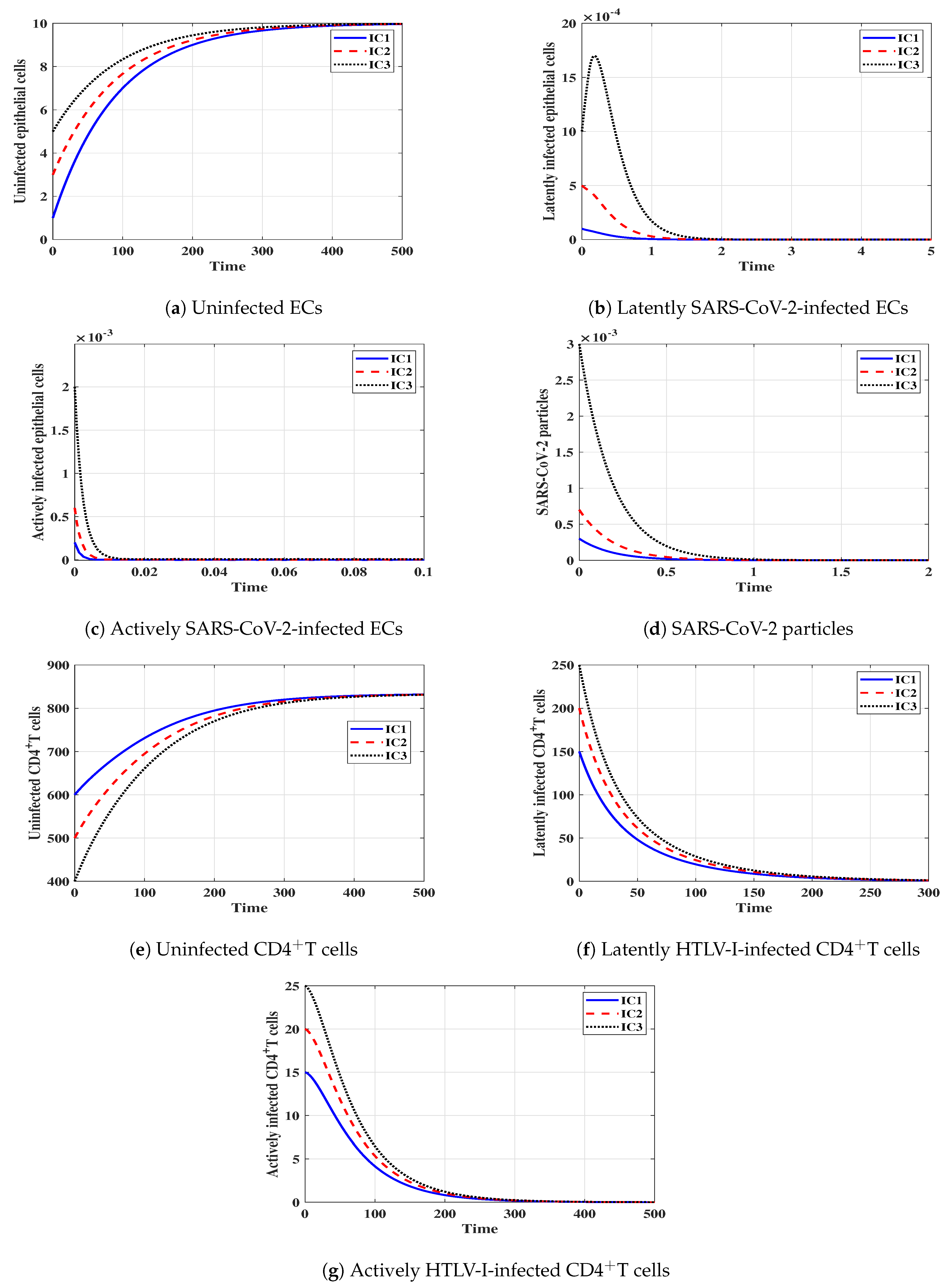
( R 1 1 and R 2 1 ): Choosing ρ = 0.8 ,   μ = 1.1 , ξ V = 5.5 and π = 0.0001 which gives R 1 = 0.2208 < 1 and R 2 = 0.0003 < 1 . Based on Theorem 1, the equilibrium point, E P 0 is GAS. This is illustrated in Figure 1, where, the concentrations of the uninfected ECs and uninfected CD4 + T cells tends to their healthy values X 0 = 10 and U 0 = 833.33 , while, the concentrations of the other compartments tend to zero. This case means the clearance of both SARS-CoV-2 and HTLV-I infections.
Case 2.
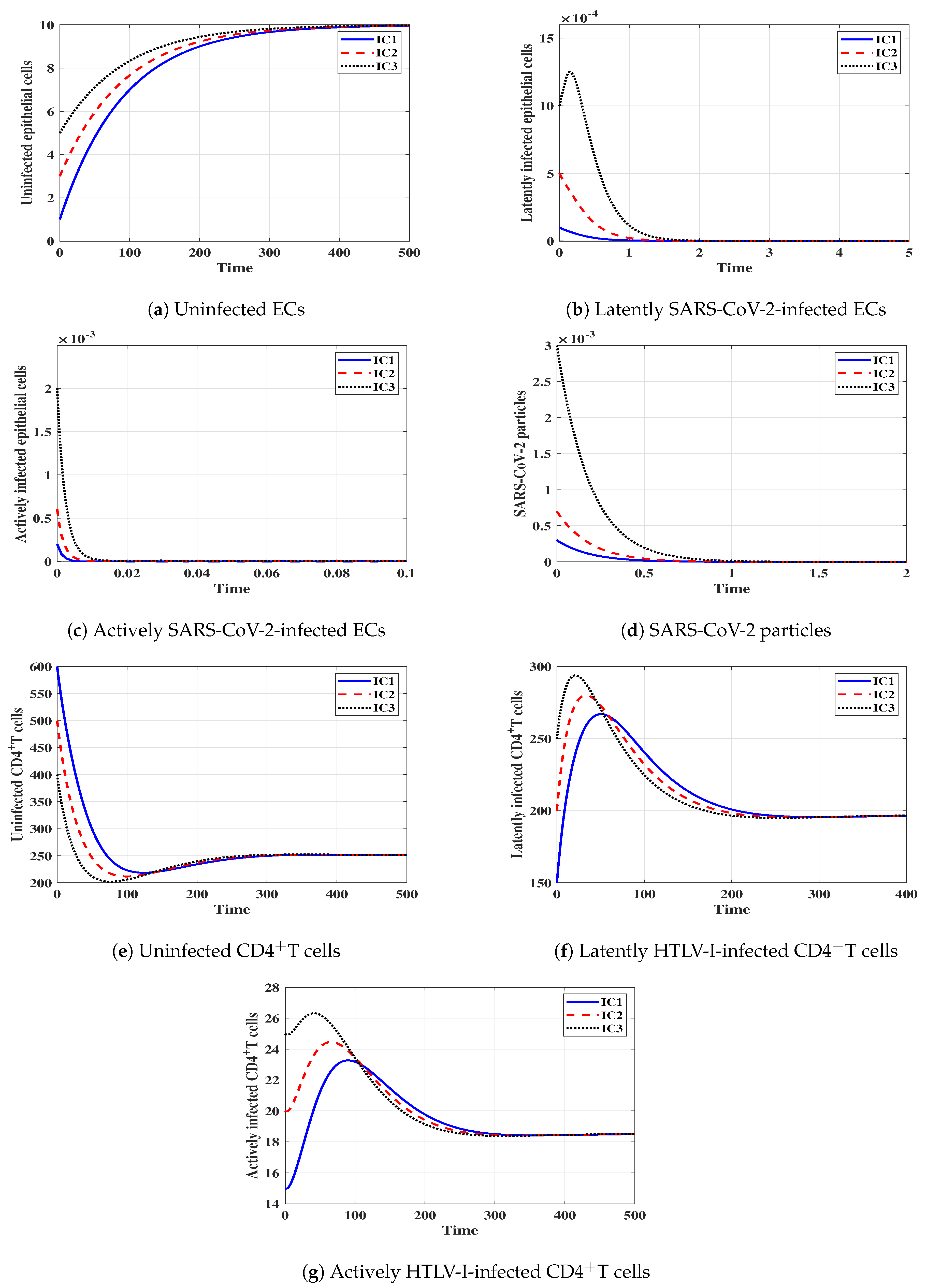
( R 1 > 1 and R 4 1 ): We take ρ = 0.5 , μ = 1.1 ,   ξ V = 5.5 and π = 0.0015 . So, we obtain R 1 = 3.3126 > 1 and R 4 = 0.0006 < 1 . According to Lemma 2 and Theorem 2, the HTLV-I mono-infection equilibrium point, E P 1 exists and is GAS. Figure 2 shows that the models’s solutions converge to the equilibrium point E P 1 = ( 10 , 0 , 0 , 0 , 251.56 , 196.97 , 18.5 ) for all initials IC1-IC3. In this situation, the patient becomes infected by HTLV-I, while the SARS-CoV-2 infection is cleared.
Case 3.
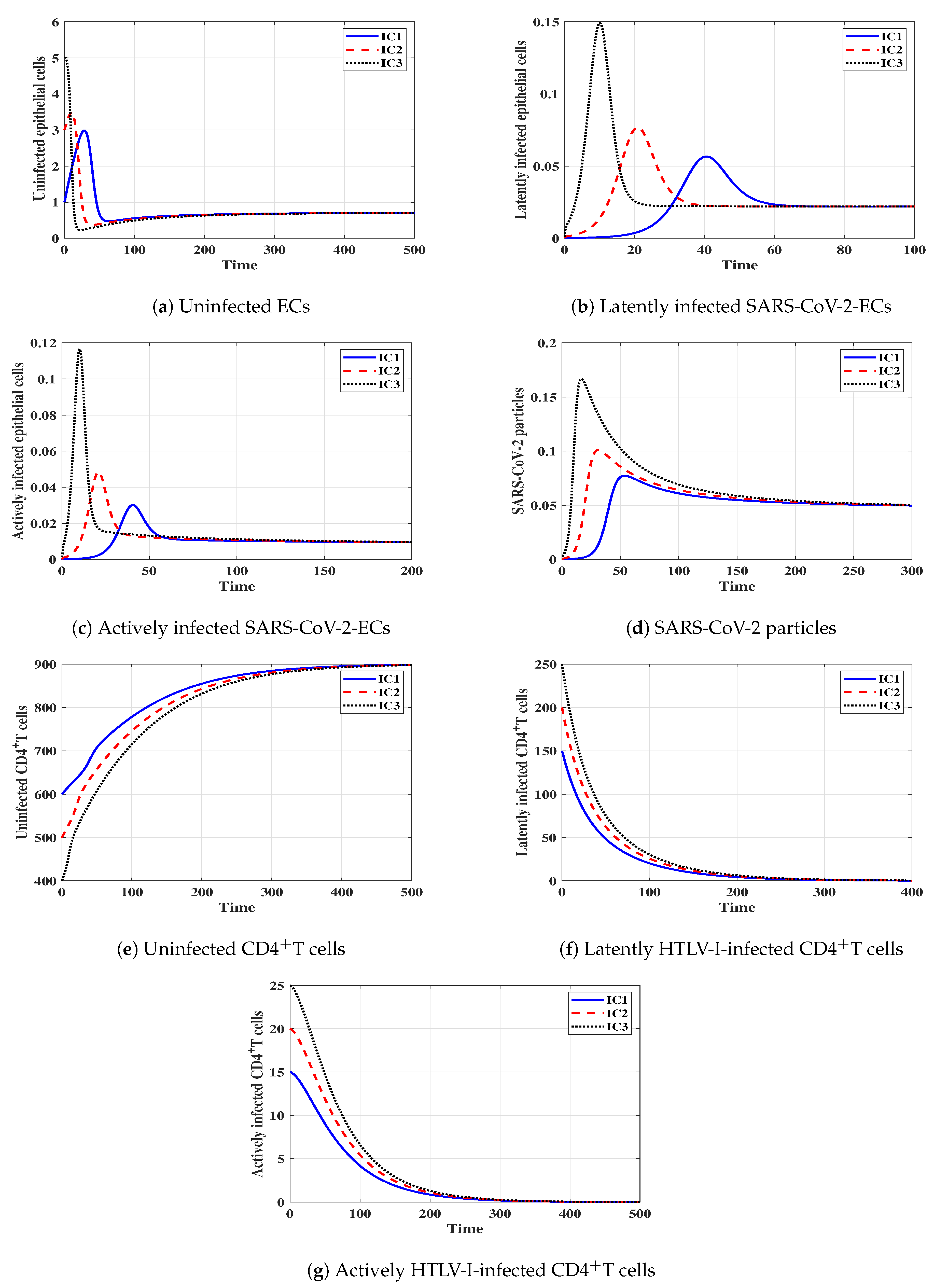
( R 2 > 1 and R 3 1 ): We choose ρ = 3 ,   μ = 0.01 , ξ V = 0.04 and π = 0.0001 . Then, we calculate R 2 = 15.3786 > 1 and R 3 = 0.2407 < 1 . Lemma 2 and Theorem 3 state that the SARS-CoV-2-mono-infection equilibrium point, E P 2 = 0.702 , 0.022 , 0.009 , 0.049 , 900.46 , 0 , 0 exists and is GAS. Figure 3 displays the numerical solutions of the system converge to E P 2 for all the three initials IC1-IC3. The results support the theoretical results presented in Theorem 3. This situation represents a patient who infected only with SARS-CoV-2.
Case 4.
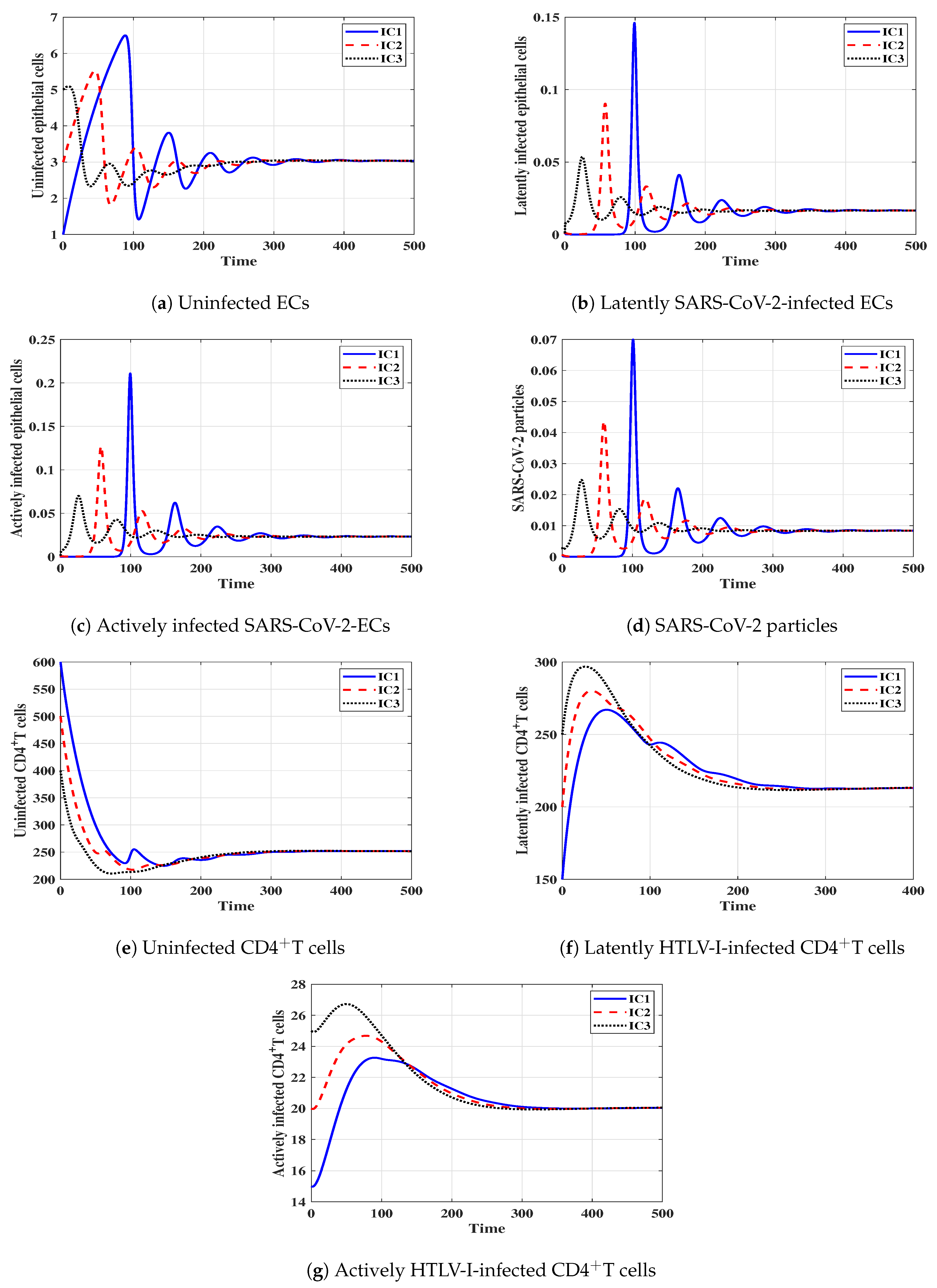
( R 4 > 1 and 1 < R 3 1 + R ˜ ): We consider ρ = 3 , μ = 0.01 , ξ V = 0.6 and π = 0.0015 . So, we obtain R 4 = 3.2969 > 1 , R 3 = 3.3113 > 1 and R 3 < 1 + R ˜ = 4.0299 . Lemma 2 and Theorem 4 state that the HTLV-I/SARS-CoV-2 coinfection E P 3 = ( 3.03 , 0.017 , 0.023 , 0.008 , 251.56 , 213.49 , 20.05 ) exists and is GAS. Figure 4 shows that the solutions of the system converge to E P 3 for all initials IC1-IC3. The results support the theoretical results presented in Theorem 4. In this case, a SARS-CoV-2 and HTLV-I coinfection happens, where a HTLV-I-patient gets contaminated with COVID-19. CD4 + T cells are animated to dispense with SARS-CoV-2 disease from the body. In any case, assuming the patient has low CD4 + T cell counts, the freedom of SARS-CoV-2 may not be accomplished. This can prompt extreme contamination and passing.

4.2. Impact of Time Delays on the Clearance of Coinfection

In this part, we study the effect of time delay parameters τ i , i = 1 , 2 , , 5 on the stability of the uninfected equilibrium point E P 0 . Since R 1 and R 2 depend on τ i ,   i = 1 , 2 , , 5 , then changing the parameters τ i will change the stability of the uninfected equilibrium point. Using the values of the parameters in Table 2 and considering ρ = 3 ,   μ = 0.01 ,   ξ V = 0.06 and π = 0.0015 to solve the model (7)–(13) with initial condition:
IC 4 : ( X ( θ ) , N ( θ ) , Y ( θ ) , V ( θ ) , U ( θ ) , L ( θ ) , A ( θ ) ) = ( 5 , 1 , 0.0012 , 0.004 , 400 , 200 , 20 ) ,
where θ max τ i , 0 , i = 1 , 2 , , 5 . Consider τ = τ 1 = τ 2 = τ 3 = τ 4 = τ 5 and the other parameters are fixed, then R 1 and R 2 can be given as functions of τ as follows:
R 1 τ = π α γ e d 4 + d 5 τ ξ U ξ L ξ A + α ξ A ε e d 5 τ , R 2 τ = δ η ρ κ ξ U e d 1 + d 2 + d 3 τ ξ X ξ V κ + ξ N ξ Y ξ U + γ μ .
We note that, when all other parameters are fixed, then R 1 and R 2 are decreasing functions of τ . Let τ c r 1 and τ c r 2 be such that R 1 τ c r 1 = R 2 τ c r 2 = 1 . Consequently,
R 1 τ 1 , for all τ τ c r 1 , R 2 τ 1 , for all τ τ c r 2 .
Therefore, E P 0 is GAS when τ τ c r 1 and τ τ c r 2 . Using the values of the parameters, we get, τ c r 1 = 0.692433 and τ c r 2 = 0.108309 . It follows that:
(i) If τ max { τ c r 1 , τ c r 2 } = 0.692433 , then R 1 τ 1 and R 2 τ 1 and thus, E P 0 is GAS.
(ii) If τ < 0.692433 , then R 1 τ > 1 or R 2 τ > 1 and thus, E P 0 will lose its stability.
Therefore, sufficiently large time delay can stabilize the system around the equilibrium E P 0 .
It is clear from Figure 5 that, as τ increases, the concentrations of the uninfected ECs and uninfected CD4 + T cells are increased, while the other concentrations of other compartments are decreased. We can see from the above discussion that increasing time delays values can have similar effect as antiviral treatments.

5. Discussion

Coinfection cases with SARS-CoV-2 and HTLV-I were reported in [3,10]. Therefore, it is important to understand the within-host dynamics of this coinfection. In this paper, we developed and examined two SARS-CoV-2 and HTLV-I coinfection models. The models considered the interactions between uninfected ECs, latently SARS-CoV-2-infected ECs, actively SARS-CoV-2-infected ECs, free SARS-CoV-2 particles, uninfected CD4 + T cells, latently HTLV-I-infected CD4 + T cells and actively HTLV-I-infected CD4 + T cells. We introduced five intracellular time delays into the models: (i) two delays in the formation of latently SARS-CoV-2-infected ECs and latently HTLV-I-infected CD4 + T cells, (ii) two delays in the reactivation of latently SARS-CoV-2-infected ECs and latently HTLV-I-infected CD4 + T cells, and (iii) maturation delay of new SARS-CoV-2 virions. Discrete-time delays and distributed-time delays were incorporated in the first and second models, respectively. We examined the nonnegativity and ultimate boundedness of the solutions. We found that these systems has four equilibria and we proved the following:
(I) The uninfected equilibrium point E P 0 always exists. It is GAS when R 1 1 and R 2 1 . In this case, the patient is recovered from both SARS-CoV-2 and HTLV-I. From a control viewpoint, making R 1 1 and R 2 1 will be a good strategy. The parameter R 2 may be reduced by multiplying the parameters by ρ or η by ( 1 ϵ 1 ) or ( 1 ϵ 2 ) , respectively. Here, ϵ 1 [ 0 , 1 ] and ϵ 2 [ 0 , 1 ] are the effectiveness of the antiviral drugs for blocking the infection and blocking the production of SARS-CoV-2 particles, respectively [20]. Since there is no treatment for HTLV-I infection [11], making R 1 1 is rarely achieved.
(II) The HTLV-I mono-infection equilibrium point, E P 1 exists if R 1 > 1 . It is GAS when R 1 > 1 and R 4 1 . This case leads to the situation of the patient who infected by HTLV-I, while the SARS-CoV-2 infection is cleared.
(III) The SARS-CoV-2 mono-infection equilibrium point, E P 2 exists if R 2 > 1 . It is GAS when R 2 > 1 and R 3 1 . This case leads to the situation of the patient who has SARS-CoV-2 mono-infection.
(IV) The HTLV-I and SARS-CoV-2 coinfection equilibrium point, E P 3 exists if R 3 > 1 and R 4 > 1 . It is GAS when R 4 > 1 and 1 < R 3 1 + R ˜ . This point represents the situation of SARS-CoV-2 and HTLV-I coinfection patient.
The global stability of equilibria was established using Lyapunov method. We performed numerical simulations and demonstrated that they are in good agreement with the theoretical results. We discussed the impact of time delays on the clearance of coinfection. We concluded that, increasing time delays values can have an antiviral treatment-like impact.
The models developed in this work can be improved by (i) utilizing real data to find a good estimation of the parameters’ values, thus, the theoretical results obtained in this paper need to be tested against empirical findings when real data become available, (ii) considering the mutations of the SARS-CoV-2, (iii) including the stochastic interaction, and (iv) considering the diffusion of cells and viruses. Future studies should evaluate the effect of SARS-CoV-2 on HTLV-1 patients. These research points need further investigations so we leave them to future works.

Author Contributions

Conceptualization, A.M.E. and A.S.S.; Formal analysis, A.M.E., A.S.S. and A.D.H.; Investigation, A.M.E. and A.S.S.; Methodology, A.M.E. and A.D.H.; Writing—original draft, A.S.S.; Writing—review & editing, A.M.E. and A.S.S. All authors have read and agreed to the published version of the manuscript.

Funding

This project was funded by the Deanship of Scientific Research (DSR), King Abdulaziz University, Jeddah, Saudi Arabia under grant no. (KEP-PHD-38-130-43).

Data Availability Statement

Not applicable.

Acknowledgments

This project was funded by the Deanship of Scientific Research (DSR), King Abdulaziz University, Jeddah, Saudi Arabia under grant no. (KEP-PHD-38-130-43). The authors, therefore, acknowledge with thanks DSR technical and financial support.

Conflicts of Interest

The authors declare no conflict of interest.

References

  1. Coronavirus Disease (COVID-19), Weekly Epidemiological Update (23 October 2022), World Health Organization (WHO). 2022. Available online: https://www.who.int/publications/m/item/weekly-epidemiological-update-on-covid-19---26-October-2022 (accessed on 15 November 2022).
  2. Coronavirus Disease (COVID-19), Vaccine Tracker, World Health Organization (WHO). 2021. Available online: https://covid19.trackvaccines.org/agency/who/ (accessed on 15 November 2022).
  3. Enomoto, T.; Shiroyama, T.; Hirata, H.; Amiya, S.; Adachi, Y.; Niitsu, T.; Noda, Y.; Hara, R.; Fukushima, K.; Suga, Y.; et al. COVID-19 in a human T-cell lymphotropic virus type-1 carrier. Clin. Case Rep. 2022, 10, e05463. [Google Scholar] [CrossRef] [PubMed]
  4. Hernandez-Vargas, E.A.; Wilk, E.; Canini, L.; Toapanta, F.R.; Binder, S.C.; Uvarovskii, A.; Ross, T.M.; Guzmán, C.A.; Perelson, A.S.; Meyer-Hermann, M. Effects of aging on influenza virus infection dynamics. J. Virol. 2014, 88, 4123–4131. [Google Scholar] [CrossRef] [PubMed] [Green Version]
  5. Zhu, X.; Ge, Y.; Wu, T.; Zhao, K.; Chen, Y.; Wu, B.; Zhu, F.; Zhu, B.; Cui, L. Co-infection with respiratory pathogens among COVID-2019 cases. Virus Res. 2020, 285, 198005. [Google Scholar] [CrossRef] [PubMed]
  6. Aghbash, P.S.; Eslami, N.; Shirvaliloo, M.; Baghi, H. Viral coinfections in COVID-19. J. Med. Virol. 2021, 93, 5310–5322. [Google Scholar] [CrossRef]
  7. Wodarz, D.; Bangham, C.R.M. Evolutionary dynamics of HTLV-I. J. Mol. Evol. 2000, 50, 448–455. [Google Scholar] [CrossRef]
  8. Human T-Lymphotropic Virus Type 1, World Health Organization (WHO). 2022. Available online: https://who.int/news-room/fact-sheets/detail/human-t-lymphotropic-virus-type-1 (accessed on 15 November 2022).
  9. Proietti, F.A.; Carneiro-Proietti, A.B.F.; Catalan-Soares, B.; Murphy, E.L. Global epidemiology of HTLV-I infection and associated diseases. Oncogene 2005, 24, 6058–6068. [Google Scholar] [CrossRef] [Green Version]
  10. Hosoba, R.; Makita, S.; Shiotsuka, M.; Kobayashi, O.; Nakano, K.; Muroya, M.; Okada, N.; Suzuki, M.; Ida, H.; Fukuhara, S.; et al. COVID-19 pneumonia in a patient with adult T-cell leukemia-lymphoma. J. Clin. Exp. Hematop. 2020, 60, 174–178. [Google Scholar] [CrossRef]
  11. Sajjadi, S.; Hejazi, S.; Ravanshad, S.; Esfehani, R.J. Human T-lymphotropic virus type 1 and novel Coronavirus Disease 2019; More complex than just a simple coinfection. Gene 2022, 834, 146550. [Google Scholar] [CrossRef]
  12. Hancioglu, B.; Swigon, D.; Clermont, G. A dynamical model of human immune response to influenza A virus infection. J. Theor. Biol. 2007, 246, 70–86. [Google Scholar] [CrossRef]
  13. Hernandez-Vargas, E.A.; Velasco-Hernandez, J.X. In-host mathematical modelling of COVID-19 in humans. Annu. Rev. Control 2020, 50, 448–456. [Google Scholar] [CrossRef]
  14. Baccam, P.; Beauchemin, C.; Macken, C.A.; Hayden, F.G.; Perelson, A. Kinetics of influenza A virus infection in humans. J. Virol. 2006, 80, 7590–7599. [Google Scholar] [CrossRef] [PubMed] [Green Version]
  15. Beauchemin, C.A.A.; McSharry, J.J.; Drusano, G.L.; Nguyen, J.T.; Went, G.T.; Ribeiro, R.M.; Perelson, A.S. Modeling amantadine treatment of influenza A virus in vitro. J. Theor. 2008, 254, 439–451. [Google Scholar] [CrossRef] [PubMed] [Green Version]
  16. Wang, S.; Pan, Y.; Wang, Q.; Miao, H.; Brown, A.N.; Rong, L. Modeling the viral dynamics of SARS-CoV-2 infection. Math. Biosci. 2020, 328, 108438. [Google Scholar] [CrossRef] [PubMed]
  17. Li, C.; Xu, J.; Liu, J.; Zhou, Y. The within-host viral kinetics of SARS-CoV-2. Math. Biosci. Eng. 2020, 17, 2853–2861. [Google Scholar] [CrossRef]
  18. Ke, R.; Zitzmann, C.; Ho, D.D.; Ribeiro, R.M.; Perelson, A.S. In vivo kinetics of SARS-CoV-2 infection and its relationship with a person’s infectiousness. Proc. Natl. Acad. Sci. USA 2021, 118, e2111477118. [Google Scholar] [CrossRef]
  19. Sadria, M.; Layton, A.T. Modeling within-host SARS-CoV-2 infection dynamics and potential treatments. Viruses 2021, 13, 1141. [Google Scholar] [CrossRef]
  20. Ghosh, I. Within host dynamics of SARS-CoV-2 in humans: Modeling immune responses and antiviral treatments. SN Comput. Sci. 2021, 2, 482. [Google Scholar] [CrossRef]
  21. Hattaf, K.; Yousfi, N. Dynamics of SARS-CoV-2 infection model with two modes of transmission and immune response. Math. Biosci. Eng. 2020, 17, 5326–5340. [Google Scholar] [CrossRef]
  22. Almoceraa, A.E.S.; Quiroz, G.; Hernandez-Vargas, E.A. Stability analysis in COVID-19 within-host model with immune response. Commun. Nonlinear Sci. Numer. 2021, 95, 105584. [Google Scholar] [CrossRef]
  23. Mondal, J.; Samui, P.; Chatterjee, A.N. Dynamical demeanour of SARS-CoV-2 virus undergoing immune response mechanism in COVID-19 pandemic. Eur. Phys. J. Spec. Top. 2022, 231, 3357–3370. [Google Scholar] [CrossRef]
  24. Gonçalves, A.; Bertrand, J.; Ke, R.; Comets, E.; De Lamballerie, X.; Malvy, D.; Pizzorno, A.; Terrier, O.; Calatrava, M.R.; Mentré, F.; et al. Timing of antiviral treatment initiation is critical to reduce SARS-CoV-2 viral load. CPT Pharmacometrics Syst. 2020, 9, 509–514. [Google Scholar] [CrossRef] [PubMed]
  25. Abuin, P.; Anderson, A.; Ferramosca, A.; Hernandez-Vargas, E.A.; Gonzalez, A.H. Characterization of SARS-CoV-2 dynamics in the host. Annu. Rev. Control 2020, 50, 457–468. [Google Scholar] [CrossRef] [PubMed]
  26. Elaiw, A.M.; Alsaedi, A.J.; Agha, A.D.A.; Hobiny, A.D. Global stability of a humoral immunity COVID-19 model with logistic growth and delays. Mathematics 2022, 10, 1857. [Google Scholar] [CrossRef]
  27. ul Rehman, A.; Singh, R.; Agarwal, P. Modeling, analysis and prediction of new variants of COVID-19 and dengue co-infection on complex network. Chaos Solitons Fractals 2021, 150, 111008. [Google Scholar] [CrossRef] [PubMed]
  28. Ojo, M.M.; Benson, T.O.; Peter, O.J.; Goufo, E.F.D. Nonlinear optimal control strategies for a mathematical model of COVID-19 and influenza co-infection. Phys. A Stat. Mech. Appl. 2022, 607, 128173. [Google Scholar] [CrossRef] [PubMed]
  29. Ringa, N.; Diagne, M.L.; Rwezaura, H.; Omame, A.; Tchoumi, S.Y.; Tchuenche, J.M. HIV and COVID-19 co-infection: A mathematical model and optimal control. Inform. Med. Unlocked 2022, 31, 100978. [Google Scholar] [CrossRef]
  30. Omame, A.; Abbas, M.; Onyenegecha, C.P. Backward bifurcation and optimal control in a co-infection model for, SARS-CoV-2 and ZIKV. Results Phys. 2022, 37, 105481. [Google Scholar] [CrossRef]
  31. Omame, A.; Abbas, M.; Abdel-Aty, A. Assessing the impact of SARS-CoV-2 infection on the dynamics of dengue and HIV via fractional derivatives. Chaos Solitons Fractals 2022, 162, 112427. [Google Scholar] [CrossRef]
  32. Mekonen, K.G.; Obsu, L.L. Mathematical modeling and analysis for the co-infection of COVID-19 and tuberculosis. Heliyon 2022, 8, e11195. [Google Scholar] [CrossRef]
  33. Pérez, A.G.; Oluyori, D.A. A model for COVID-19 and bacterial pneumonia coinfection with community-and hospital-acquired infections. arXiv 2022, arXiv:2207.13265. [Google Scholar] [CrossRef]
  34. Zhou, Y.; Huang, M.; Jiang, Y.A.; Zou, X. Data-driven mathematical modeling and dynamical analysis for SARS-CoV-2 coinfection with bacteria. Int. J. Bifurc. Chaos 2021, 31, 2150163. [Google Scholar] [CrossRef]
  35. Elaiw, A.M.; Agha, A.D.A.; Azoz, S.A.; Ramadan, E. Global analysis of within-host SARS-CoV-2/HIV coinfection model with latency. Eur. Phys. J. Plus 2022, 137, 174. [Google Scholar] [CrossRef] [PubMed]
  36. Agha, A.D.A.; Elaiw, A.M. Global dynamics of SARS-CoV-2/malaria model with antibody immune response. Math. Eng. 2022, 19, 8380–8410. [Google Scholar] [CrossRef] [PubMed]
  37. Elaiw, A.M.; Alsulami, R.S.; Hobiny, A.D. Modeling and stability analysis of within-host IAV/SARS-CoV-2 coinfection with antibody immunity. Mathematics 2022, 10, 4382. [Google Scholar] [CrossRef]
  38. Kharitonov, V.L. Time-Delay Systems: Lyapunov Functionals and Matrices; Springer Science & Business Media: Berlin/Heidelberg, Germany, 2012. [Google Scholar]
  39. Lu, X.; Li, H.; Zhang, X. Positivity and stability of timescale-type linear singular systems with time delays. Sci. Inf. Sci. 2022, 65, 1–16. [Google Scholar] [CrossRef]
  40. Li, Y.; Li, H.; Ding, X. Set stability of switched delayed logical networks with application to finite-field consensus. Automatica 2020, 113, 108768. [Google Scholar] [CrossRef]
  41. Juárez, L.; Mondié, S.; Kharitonov, V.L. Dynamic predictor for systems with state and input delay: A time-domain robust stability analysis. Int. J. Robust Nonlinear Control 2020, 30, 2204–2218. [Google Scholar] [CrossRef]
  42. Nath, B.J.; Dehingia, K.; Mishra, V.N.; Chu, Y.-M.; Sarmah, H.K. Mathematical analysis of a within-host model of SARS-CoV-2. Adv. Differ. Equ. 2021, 2021, 113. [Google Scholar] [CrossRef]
  43. Stilianakis, N.I.; Seydel, J. Modeling the T-cell dynamics and pathogenesis of HTLV-I infection. Bull. Math. Biol. 1999, 61, 935–947. [Google Scholar] [CrossRef] [Green Version]
  44. Katri, P.; Ruan, S. Dynamics of human T-cell lymphotropic virus I (HTLV-I) infection of CD4+T cells. Comptes Rendus Biol. 2004, 327, 1009–1016. [Google Scholar] [CrossRef]
  45. Pan, X.; Chen, Y.; Shu, H. Rich dynamics in a delayed HTLV-I infection model: Stability switch, multiple stable cycles, and torus. J. Math. Anal. Appl. 2019, 479, 2214–2235. [Google Scholar] [CrossRef]
  46. Li, M.Y.; Shu, H. Multiple stable periodic oscillations in a mathematical model of CTL response to HTLV-I infection. Bull. Math. Biol. 2011, 73, 1774–1793. [Google Scholar] [CrossRef] [PubMed]
  47. Wang, L.; Liu, Z.; Li, Y.; Xu, D. Complete dynamical analysis for a nonlinear HTLV-I infection model with distributed delay, CTL response and immune impairment. Discret. Contin. Dyn. 2020, 25, 917–933. [Google Scholar] [CrossRef] [Green Version]
  48. Muroya, Y.; Enatsu, Y.; Li, H. Global stability of a delayed HTLV-I infection model with a class of nonlinear incidence rates and CTLs immune response. Appl. Math. Comput. 2013, 219, 10559–10573. [Google Scholar] [CrossRef]
  49. Li, F.; Ma, W. Dynamics analysis of an HTLV-1 infection model with mitotic division of actively infected cells and delayed CTL immune response. Math. Methods Appl. Sci. 2018, 41, 3000–3017. [Google Scholar] [CrossRef]
  50. Li, S.; Zhou, Y. Backward bifurcation of an HTLV-I model with immune response. Discret. Contin. Dyn. Syst. Ser. B 2016, 21, 863–881. [Google Scholar]
  51. Li, M.Y.; Lim, A.G. Modelling the role of Tax expression in HTLV-1 persisence in vivo. Bull. Math. Biol. 2011, 73, 3008–3029. [Google Scholar] [CrossRef]
  52. Lim, A.G.; Maini, P.K. HTLV-I infection: A dynamic struggle between viral persistence and host immunity. J. Theoretical Biol. 2014, 352, 92–108. [Google Scholar] [CrossRef] [Green Version]
  53. Khajanchi, S.; Bera, S.; Roy, T.K. Mathematical analysis of the global dynamics of a HTLV-I infection model, considering the role of cytotoxic T-lymphocytes. Math. Comput. Simul. 2021, 180, 354–378. [Google Scholar] [CrossRef]
  54. Bera, S.; Khajanchi, S.; Roy, T.K. Dynamics of an HTLV-I infection model with delayed CTLs immune response. Appl. Math. Comput. 2022, 430, 127206. [Google Scholar] [CrossRef]
  55. Wang, W.; Ma, W. Global dynamics of a reaction and diffusion model for an HTLV-I infection with mitotic division of actively infected cells. J. Appl. Anal. Comput. 2017, 7, 899–930. [Google Scholar] [CrossRef]
  56. Elaiw, A.M.; AlShamrani, N.H. Analysis of a within-host HIV/HTLV-I co-infection model with immunity. Virus Res. 2021, 295, 198204. [Google Scholar] [CrossRef]
  57. Bellomo, N.; Burini, D.; Outada, N. Multiscale models of COVID-19 with mutations and variants. Netw. Heterog. Media 2022, 17, 293–310. [Google Scholar] [CrossRef]
  58. Zhou, X.; Zhang, L.; Zheng, T.; Li, H.; Teng, Z. Global stability for a delayed HIV reactivation model with latent infection and Beddington-DeAngelis incidence. Appl. Math. Lett. 2021, 117, 107047. [Google Scholar] [CrossRef]
  59. Elaiw, A.M.; AlShamrani, N.H. Stability of HIV/HTLV-I co-infection model with delays. Math. Appl. Sci. 2022, 45, 238–300. [Google Scholar] [CrossRef]
  60. Hale, J.K.; Lunel, S.V. Introduction to Functional Differential Equations; Springer: New York, NY, USA, 1993. [Google Scholar]
  61. Korobeinikov, A. Global properties of basic virus dynamics models. Bull. Math. Biol. 2004, 66, 879–883. [Google Scholar] [CrossRef]
  62. Barbashin, E.A. Introduction to the Theory of Stability; Wolters-Noordhoff: Groningen, The Netherlands, 1970. [Google Scholar]
  63. LaSalle, J.P. The Stability of Dynamical Systems; SIAM: Philadelphia, PA, USA, 1976. [Google Scholar]
  64. Lyapunov, A.M. The General Problem of the Stability of Motion; Taylor & Francis, Ltd.: London, UK, 1992. [Google Scholar]
  65. Prakash, M.; Rakkiyappan, R.; Manivannan, A.; Cao, J. Dynamical analysis of antigen-driven T-cell infection model with multiple delays. Appl. Math. Comput. 2019, 354, 266–281. [Google Scholar] [CrossRef]
  66. Pinky, L.; Dobrovolny, H.M. SARS-CoV-2 coinfections: Could influenza and the common cold be beneficial? J. Med. Virol. 2020, 92, 2623–2630. [Google Scholar] [CrossRef]
  67. Asquith, B.; Bangham, C.R.M. Quantifying HTLV-I dynamics. Immunol. Cell Biol. 2007, 85, 280–286. [Google Scholar] [CrossRef]
  68. Perelson, A.S.; Kirschner, D.E.; Boer, R.D. Dynamics of HIV Infection of CD4+T cells. Math. Biosci. 1993, 114, 81–125. [Google Scholar] [CrossRef]
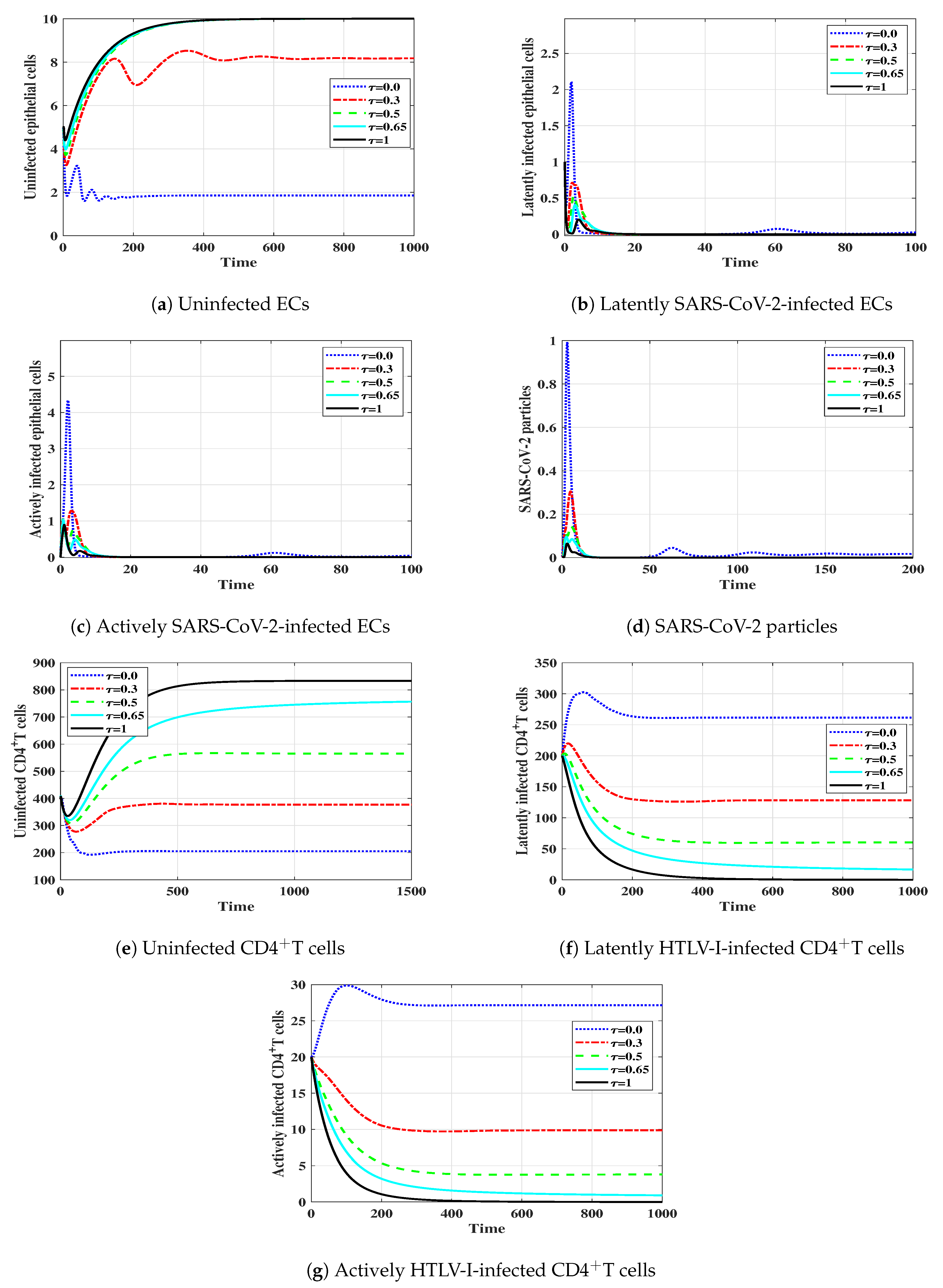
Figure 1. Solutions of system (7)–(13) with initial conditions IC1–IC3 in Case 1.
Mathematics 10 04756 g001
Figure 2. Solutions of system (7)–(13) with initial conditions IC1–IC3 in Case 2.
Mathematics 10 04756 g002
Figure 3. Solutions of system (7)–(13) with initial conditions IC1–IC3 in Case 3.
Mathematics 10 04756 g003
Figure 4. Solutions of system (7)–(13) with initial conditions IC1–IC3 in Case 4.
Mathematics 10 04756 g004
Figure 5. Impact of time delays parameters τ i , i = 1 , 2 , 3 , 4 , 5 on the HTLV-I/SARS-COV-2 coinfection’s dynamics given by system (7)–(13) with initial conditions IC4.
Mathematics 10 04756 g005
Table 1. Conditions of existence and global stability of the system’s equilibria.
Equilibrium PointExistence ConditionsGlobal Stability Conditions
E P 0 = X 0 , 0 , 0 , 0 , U 0 , 0 , 0 None R 1 1 and R 2 1
E P 1 = X 1 , 0 , 0 , 0 , U 1 , L 1 , A 1 R 1 > 1 R 1 > 1 and R 4 1
E P 2 = X 2 , N 2 , Y 2 , V 2 , U 2 , 0 , 0 R 2 > 1 R 2 > 1 and R 3 1
E P 3 = X 3 , N 3 , Y 3 , V 3 , U 3 , L 3 , A 3 R 3 > 1 and R 4 > 1 R 4 > 1 and 1 < R 3 1 + R ˜
Table 2. Model parameters.
ParameterValueSourcesParameterValueSources
δ 0.11 [26]u 0.1 [35,65]
ξ X 0.011 [26] ξ U 0.012 [49,51,52]
ρ VariesAssumed π VariesAssumed
κ 4.08 [35,66] ω 0.9 [50]
ξ N 0.11 [26] ε * 0.011 [50]
ξ Y 0.11 [35,42] α 0.003 [49,51,52,67]
μ VariesAssumed ξ L 0.03 [50,51,52,53]
η 0.24 [35] ξ A * 0.03 [49,51,52]
ξ V VariesAssumed d i , i = 1 , , 5 1.0 Assumed
γ 10[51,52,68] τ i , i = 1 , , 5 VariesAssumed
Publisher’s Note: MDPI stays neutral with regard to jurisdictional claims in published maps and institutional affiliations.