Abstract
The issuance of multiple-event catastrophe bonds (MECBs) has the potential to increase in the next few years. This is due to the increasing trend in the frequency of global catastrophes, which makes single-event catastrophe bonds (SECBs) less relevant. However, there are obstacles to issuing MECBs since the pricing framework is still little studied. Therefore, this study aims to develop such a new pricing framework. The model uniquely involves three new variables: the trigger event correlation, interest, and inflation rates. The trigger event correlation rate was accommodated by the involvement of the copula while the interest and inflation rates were simultaneously considered using an integrated autoregressive vector stochastic model. After the model was obtained, the model was simulated on storm catastrophe data in the United States. Finally, the effect of the three variables on MECB prices was also analyzed. The analysis results show that the three variables make MECB prices more fairly than other models. This research is expected to guide special purpose vehicles to set fairer MECB prices and can also be used as a reference for investors in choosing MECBs based on the rates of trigger event correlation and the real interest they can expect.
Keywords:
multiple-event catastrophe bond; trigger event correlation rate; interest rate; inflation rate; copula; integrated autoregressive vector MSC:
91B70; 91B84; 91G15; 91G20; 91G30
1. Introduction
The design of special mechanisms regarding postcatastrophe financing by countries in the world has been a serious concern in the last 30 years [1,2]. This is intended so that the catastrophe risk in these countries can be minimized, and catastrophe recovery can be quickly carried out. One of these efforts is through the insurance-linked securities (ILS) scheme, where the country’s catastrophe risk is transferred to investors via financial securities in the capital market [3]. One of the most successful ILS is the catastrophe bond (cat bond) [4,5]. The cat bond can raise significant funds quickly with moderate financial risk. The cat bond was first published by Hannover RE in 1994 [6,7,8]. Then, another cat bond was issued in 2006 by Mexico, which was devoted to shifting the risk of earthquake catastrophe [9,10]. The issuance prompted other Caribbean countries to use the cat bond in financing the catastrophe contingency of earthquakes and hurricanes in 2014 [11,12].
Along with the increasing tendency of catastrophe frequency, the single-event catastrophe bond (SECB) has the potential to be less attractive to investors [13]. This occurs because the probability that a single claim-triggering event will happen is more significant. So, the risk that investors will lose their principal is also higher. To address this, the Organization for Economic Cooperation and Development (OECD) [14] suggested issuing a multiple-event catastrophe bond (MECB). The same suggestion was also expressed by Woo [15]. MECBs can lower investors’ probability of losing their principal [16]. This is because the loss of principal of an investor occurs when several separate trigger events have occurred. Then, the expected profit from MECBs is also higher than SECBs [17]. Unfortunately, there are obstacles to issuing these securities since the pricing framework is still little studied. This is because this type of MECB is still very new.
Several studies have examined the pricing framework of the MECB. They are Reshetar [16], Sun et al. [18], Chao and Zou [19], Ibrahim et al. [20], and Wei et al. [21]. Briefly, an overview of these studies is presented in Table 1.

Table 1.
The previous studies on the design of the MECB pricing framework.
Table 1 shows that the trigger event indices commonly used in designing MECB pricing frameworks in previous studies are the loss and fatality indices, where three out of five used them. Only Sun et al. [18] and Wei et al. [21] used long-term and short-term rainfall indices and magnitude and loss indices, respectively. Then, the primary methods used vary. Copula, compound Poisson process, and Monte Carlo methods are commonly used. Then, four of the five models involved the trigger event correlation rate. Only Ibrahim et al. [20] did not apply it. Finally, all authors preferred a stochasticity of the interest rate over constancy. This was done so the model was more in line with an actual situation where the interest rate fluctuates year by year. Finally, all models did not consider the stochasticity of the inflation rate.
The gaps from previous studies are discussed in this paragraph. Of the five studies presented in Table 1, there is no study involving the stochasticity of the inflation rate. This factor is crucial to involve so that investors get the expected real interest rate following market fluctuations. If the inflation rate is higher than the interest rate, then the real interest rate earned by investors is lower than expected and vice versa [23,24].
Based on the previous gaps described, this study aims to develop an MECB pricing framework that involves the stochasticity of the inflation rate. This study also involves other variables, such as the trigger event correlation rate and the stochasticity of the interest rate. The trigger event indices used were loss and fatality. Both indices were used because they are common measures to financially and nonfinancially measure the severity of all catastrophe types [16,20]. The indices of loss and fatality can describe losses in terms of property and demographics of a country, respectively. Then, to consider the trigger event correlation rate, we used copulas in the joint-risk measurement of two trigger events. Next, to model the stochasticity of inflation and interest rates efficiently, we carried out an autoregressive integrated vector model. After the model was designed, a simulation was conducted on storm catastrophe data in the United States. Finally, the effect of the rates of trigger event correlation, interest, and inflation on MECB prices was also analyzed. This research is expected to guide special purpose vehicles to sets fairer MECB prics and can also be used as a reference for investors in choosing MECBs based on the rates of trigger event correlation and real interest they can expect.
2. The Literature Review
So far, SECB price modeling has been studied more than MECB price modeling. Zimbidis et al. [25] proposed the earthquake SECB pricing model designed via the extreme value approach (EVA). This model was simulated using stochastic iteration and Monte Carlo on earthquake data in Greece. Then, Nowak and Romaniuk [26] designed an SECB pricing model with an assumption of independence between dynamic interest rates and catastrophic risks using the Cox–Ingersoll–Ross (CIR) and Hull–White models. Jarrow [22] modeled SECB prices in a simple closed form via a robust model. Then, in their research, Nowak and Romaniuk [27] proposed an SECB pricing model designed using a jump-diffusion process and a multifactor CIR model. Liu et al. [28] designed an SECB pricing model by considering credit risk factors via the Jarrow and Turnbull methods. Then, Ma and Ma [29] designed a no closed-form SECB price model using the compound Poisson process. The model solution was sought by a new approximation method introduced by Chaubey et al. [30]. Tang and Yuan [31] introduced integration between distortion and neutral risk of probability measures in SECB price modeling in their research. Ma et al. [32] modeled an SECB price whose characteristics of catastrophe are accommodated via the integration of the Black Derman Toy model and the doubly-stochastic Poisson process.
Until this article was written, five studies focused on MECB price modeling. MECB price modeling was first carried out by Reshetar [16]. The model considered losses, fatalities, stochastic interest rates, and trigger event correlation rates and was designed using a representative agent pricing model and copula. Then, Sun et al. [18] introduced the drought MECB pricing model by considering the long-term and short-term rainfall and the stochasticity of interest rates. This model is a development of the Jarrow model with an addition of more triggers. Then, Chao and Zou [19] developed the Reshetar [16] model by adding catastrophe intensity through a homogeneous compound Poisson process. Then, Ibrahim et al. [20] proposed a no closed-form solution model of MECB price through continuous distribution approximation and Nuel recursive methods. These two methods are new and computationally efficient in finding model solutions. Finally, Wei et al. [21] modeled an earthquake MECB price via a homogeneous compound Poisson process, EVA, and copula. The model is the first MECB earthquake model that includes loss and magnitude of earthquake as triggers for its claims. From these five studies, no MECB price modeling involves the stochasticity of the inflation rate, the trigger event correlation rate, and the stochasticity of the interest rate. It is a novelty and is carried out in this study.
3. A Brief MECB Explanation
An MECB is an insurance-linked bond with two claim trigger events. Although this appears detrimental to the insured, it is not [14,15]. The reason is the increasing trend of worldwide catastrophe frequency, which is predicted to occur in the future. In this situation, investors’ interest in sharing country catastrophe risk via SECBs will decline because the probability of an SECB’s trigger event occurring is higher than before. If the trigger event occurs, the investor will lose the partial principal and the total coupon. To overcome this, MECBs can be a solution because the investor loses partial principal and the entire coupon when two separate trigger events occur. It can increase investors’ interest in their involvement with country catastrophe risk-sharing [16,20].
The simple structure of catastrophe risk securitization via MECB is visually presented in Figure 1.
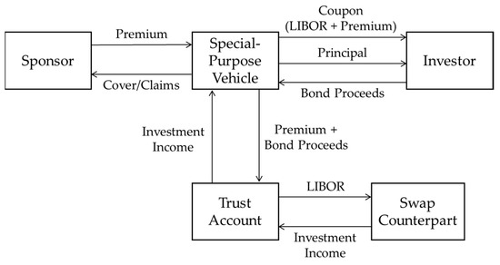
Figure 1.
The simple structure of MECB.
Figure 1 shows three main entities in the structure of catastrophe risk securitization via MECB: sponsors, special purpose vehicles (SPV), and investors [33]. The sponsor (government, insurer, or reinsurer) submits a catastrophe risk transfer contract to the SPV. After that, the sponsor also pays a premium to the SPV in exchange for the transfer. After the contract is signed and the premium is paid, the SPV issues the MECB. The MECB proceeds received from investors and the premium are invested in safe short-term financial securities [29]. The income of the investment is then deposited in a trust account. To increase the immunity of sponsors and investors from risks of default and interest rates, the SPV converts the income in the trust account into floating interest rate swap payments based on the London interbank offered rate (LIBOR) [5,34]. If one of the trigger events occurs within the MECB term, the coupon payments to investors are terminated. Then, if two trigger events occur within the MECB term, the principal is not paid to the investor in total [35]. Finally, if two trigger events do not happen within the MECB term, the coupon and principal are paid in-full to the investor.
4. Pricing Framework
4.1. Notations in Modeling
The notations used in designing MECB price model in this study are as follows:
- (a)
- is an integer greater than zero representing the MECB term in years.
- (b)
- represents the principal of the MECB which is paid at maturity.
- (c)
- represents the coupon paid in year .
- (d)
- is the catastrophe frequency that occurs until time in the area stated in the MECB contract.
- (e)
- represents the -th catastrophe loss that occurs in the area stated in the MECB contract.
- (f)
- represents the number of fatalities of the -th catastrophe that occurs in the area stated in the MECB contract.
- (g)
- represents the catastrophe loss aggregate until time .
- (h)
- represents the catastrophe fatality aggregate until time .
- (i)
- represents the correlation rate of trigger events.
- (j)
- represents the attachment point of the catastrophe loss aggregate.
- (k)
- represents the attachment point of the catastrophe fatality aggregate.
- (l)
- represents the first time the catastrophe loss aggregate exceeds its attachment points.
- (m)
- represents the first time the catastrophe fatality aggregate exceeds its attachment points.
- (n)
- represents the first time one of the catastrophe loss or fatality aggregates exceeds the attachment point.
- (o)
- represents the first time the catastrophe loss and fatality aggregates exceed the attachment point.
- (p)
- represents the annual real interest rate in year .
- (q)
- represents the annual nominal interest rate in year .
- (r)
- represents the annual inflation rate in year .
- (s)
- represents the zero-coupon MECB price with a term of year.
- (t)
- represents the coupon-paying MECB price with a term of year.
4.2. The Compound Poisson Process in Modeling Loss and Fatality Aggregates
The catastrophe loss and fatality aggregates in this study were used as measures of catastrophe severity. Loss and fatality aggregates represented by a compound Poisson process are respectively expressed as follows:
and
where represents a homogeneous Poisson process with intensity . In addition, and are assumed to be independent of . The cumulative distribution functions (CDFs) of the loss and fatality aggregates are respectively expressed as follows [36,37]:
and
Then, the survival distribution functions (SDFs) of the loss and fatality aggregates are respectively expressed as follows [36,37]:
and
The joint CDF and SDF of the loss and fatality aggregates are respectively expressed as follows [38]:
and
4.3. Trigger Events
In this study, the two trigger events of an MECB were defined as the first time the loss and fatality aggregates exceed their attachment points. The first time the loss aggregate exceeds its attachment point is mathematically expressed as follows:
Note that , and [39]. Meanwhile, the first time the fatality aggregate exceeds its attachment point is mathematically expressed as follows:
Note that , and [39].
The joint CDF of two trigger events is modeled as follows [16,38]:
Then, the joint SDF of trigger events is modeled as follows [16,38]:
4.4. The Copula in Modeling the Joint Distribution of Trigger Events
The joint CDF and SDF of trigger events in Equations (11) and (12) can each be transformed into copula form by substituting into the copula function as follows [38]:
and
It must be noted that the copula function is unique only in its domain.
Several copula families can be used to represent the copula function . The extreme values of catastrophe loss and fatality aggregates generally have a heavy right-tail probability distribution [29]. This is because these events are rare. Therefore, the copula used must precisely measure two extreme events’ probability simultaneously. These copulas are those of the Archimedean family [16,19,40,41]. Some of the copulas of the Archimedean family that we considered were Clayton, Gumbel, Frank, and Joe. in Equations (13) and (14), which are expressed in copulas of Clayton, Gumbel, Frank, and Joe, are respectively stated as follows:
and
To estimate the copula parameter , the Kendall tau () inversion method was used. This method is practical because the parameter is evaluated through its relationship to the Kendall tau [16]. The Kendall tau is the correlation rate of trigger events. Based on (13) and (14), the correlation rate of trigger events is equivalent to the correlation rates of the loss and fatality aggregates [16,19]. The relationship between and of the copulas of Clayton, Gumbel, and Frank are, respectively, stated as follows [41]:
and
No closed form can express the relationship between and in Joe’s copula. As an alternative, numerical methods were used to determine the parameter.
4.5. The Annual Real Interest Rate Dynamics
The annual real interest rate is the interest rate obtained after considering the inflation rate. This study used it to determine the present value of the principal and coupon payments of the MECB. Mathematically, the present value of one unit of currency in the next years is expressed as follows [42]:
where
[43]. In this study, is depicted through and simultaneous modeling with an integrated autoregressive vector model. Mathematically, the integrated autoregressive vector model of and is expressed as follows [44,45]:
where represents a two-dimensional vector containing and that has been differentiated times, represents the order of the integrated autoregressive vector model, with , represents the coefficient matrix of , and represents the residual random vectors. This model assumes that is a stationary random vector sequence, and is independent and normally bivariate distributed with a zero vector mean and constant covariance matrix as the variance [46].
4.6. The Formulation of Zero-Coupon MECB Price Model
The principal payment structure of a zero-coupon MECB was designed in advance. The principal of a zero-coupon MECB is proportionally paid the first time the loss and fatality aggregates exceed their attachment point within the zero-coupon MECB term. Mathematically, the first time the loss and fatality aggregates exceed their attachment point is stated as follows:
Then, if the loss and fatality aggregates do not exceed their attachment point within the zero-coupon MECB term, the principal paid to investors on the maturity date is intact. Mathematically, the principal payment structure to investors on the maturity date is expressed as follows:
where expresses the principal of the zero-coupon MECB, and is a real number in the real interval expressing the proportion of principal payments. The zero-coupon MECB price is modeled as the present value of the MECB principal’s expectation at maturity. Mathematically, the zero-coupon MECB price model is expressed in the following equation:
Proof.
See Appendix A. □
4.7. The Formulation of Coupon-Paying MECB Price Model
The annual coupon payment structure of an MECB was designed in advance. Coupons of coupon-paying MECB are terminated the first time one of the losses or fatalities aggregates exceeds their attachment point within the coupon-paying MECB term. The first time one of the losses or fatalities aggregates exceeds the attachment point is stated as follows:
Then, if the loss and fatality aggregates do not exceed their attachment point within the coupon-paying MECB term, the coupon is paid in full to investors every year. Mathematically, the structure of annual coupon payments to investors is expressed in the following equation:
where represents the annual coupon payment. Meanwhile, the principal payment structure from the MECB to investors at maturity () is the same as Equation (26). The coupon-paying MECB price is modeled as the total of the present value of the expected annual coupon payments and the expected principal at maturity. Mathematically, the coupon-paying MECB price is expressed in the following equation:
Proof.
See Appendix B. □
5. Simulation
5.1. Overview of Data
The simulation data used were as follows:
- (a)
- Data on adjusted nonzero single storm catastrophe losses in the United States from 2012 to 2021.
- (b)
- Data on the number of nonzero single storm catastrophe fatalities in the United States from 2012 to 2021.
- (c)
- Data on storm catastrophe frequency in the United States from 1980 to 2021.
- (d)
- Data on adjusted annual losses and fatalities from storm catastrophes in the United States from 1980 to 2021.
- (e)
- Data on the annual federal reserve and inflation rates in the United States from 1979 to 2021.
Data (a) to (d) can be accessed on the International Disaster Database (https://www.emdat.be accessed on 14 February 2022). Meanwhile, data (e) can be accessed at the World Bank (https://data.worldbank.org/ accessed on 30 July 2022). Data (a) to (b) are also used in Ibrahim et al. [20], and the obtained conclusions are as follows:
- (a)
- The random variable , which is the -th catastrophe loss, follows the Weibull distribution with shape parameter and scale parameter .
- (b)
- The random variable , which is the number of fatalities of the -th catastrophe, follows the Geometric distribution with parameter .
- (c)
- The Skewness of is 3.2973.
Then, from data (c), we obtained that the storm catastrophe intensity in the United States is per year. Finally, from data (a), (c), and (d), we obtained the kurtosis of the loss aggregate for are 1.0885, 0.5443, and 0.3628, respectively.
5.2. Modeling the Copula of the Trigger Events
The first step was estimating the copula parameter. We used the Kendall tau () inversion method to estimate it. To simplify the estimation, we used the help of the R software through the “VineCopula” package [47]. Briefly, the parameter estimation results are presented in Table 2.
Table 2.
The parameter estimators and KS statistical test value of copulas.
After the copula parameter estimators were obtained, next was selecting the fittest copula to measure the joint risk of trigger events. This study used the Kolmogorov–Smirnov (KS) statistical test with a significance level of 0.05. The selected copula was the copula that had the smallest KS statistical test value [16,19]. To determine each value of the KS statistical test of the copula, we used the help of the R software via the “VineCopula” package [47]. The KS statistical test value of each copula is also presented in Table 2. Table 2 shows that all KS statistical values of each copula are less than the critical value of 0.2052. In other words, the four copulas fit the empirical copula. The most fit is the Clayton copula because the KS statistical test value is smaller than the others. Thus, the Clayton copula was chosen as the fittest copula to describe the joint risk of trigger events. Visually, from Figure 2, the probability–probability plot (PP plot) of the Clayton copula also appears to coincide with a straight line than the other copula PP plots.
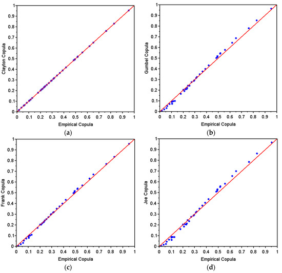
Figure 2.
PP Plots of Clayton (a), Gumbel (b), Frank (c), and Joe (d) copulas.
5.3. Modeling Real Interest Rate with Integrated Autoregressive Vector Model
To simplify the modeling of and with the integrated autoregressive vector model, we used the help of the R software through the “tseries” and “MTS” packages [48,49]. The first step was checking the stationarity of and in the mean and variance. The stationarity tests in the mean and variance were carried out using the Augmented Dicky–Fuller (ADF) test with a significance level of 0.01 and the Box–Cox parameter test, respectively. In short, and have the same p-values for the ADF test, 0.009. The two p-values are less than 0.01, so each time series was stationary in the mean. Then, and also have the same value for the Box–Cox parameter, 1.9999. The two Box–Cox parameter values are greater than 1, so each time series was stationary in variance.
After checking stationarity, next was selecting the autoregressive order. The selection was conducted via a cross-correlation diagram. The chosen order was the lag that was cut off in the diagram. The maximum order considered in this study was 10. The cross-correlation diagram of each lag is presented in Figure 3.
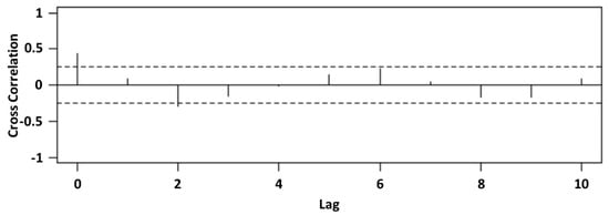
Figure 3.
The cross-correlation diagram.
Figure 3 shows that the cross-correlation diagram was cut off at lag two. In other words, the fittest autoregressive order was two. In addition to the cross-correlation diagram, selecting the autoregressive order was also conducted via the Akaike information criterion (AIC), Bayesian information criterion (BIC), and Hannan–Quinn information criterion (HQIC). The order with the smallest AIC, BIC, and HQIC values was selected [50]. Briefly, from Table 3, the smallest AIC, BIC, and HQIC values are on order two. This order is the same as obtained via the cross-correlation diagram. Based on this, the order integrated autoregressive vector model used was two.
Table 3.
The AIC BIC, and HQIC values of the integrated autoregressive model with order one to ten.
Next was estimating the parameter of the model. The estimation was carried out using the least squares (LS) method. In short, the parameter estimator results are and . After estimating the parameters, the next step was checking the assumption that is normally bivariate distributed with a zero vector mean and constant covariance matrix as the variance. The bivariate normality test used was the Henze–Zirkler (HZ) test with a significance level of 0.01. In short, the p-value of this test is 0.0112. It is greater than 0.01. In other words, is normally bivariate distributed with a zero vector mean and constant covariance matrix as the variance. Then, to check the independence of , we used the Ljung–Box test with a significance level of 0.01. In short, the p-value of this test is 0.9300. It is greater than 0.01. In other words, is independent. Finally, the practical forecasting of and for the next three years was carried out. After the model was transformed into the original data, the forecast results from and are presented in Table 4. The forecast results are used in the MECB pricing in Section 5.5.
Table 4.
The forecast results from and for the next three years.
Table 4 shows that the predicted nominal interest rate for the next three years is lower than the inflation rate. In other words, the real interest rate is also negative for the next three years. This is not strange and not the first time this has happened, as seen in Figure 4. Negative real interest rates indicate that the purchasing power of the public is experiencing a decline [51].
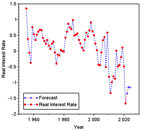
Figure 4.
Real interest rates and forecasts.
5.4. Numerical Methods for Simulation
The MECB price model in Equations (27) and (30) is difficult to solve analytically. This is because the CDF values of and are challenging to calculate. Therefore, the CDF values of and were calculated using the gamma inverse-Gaussian (GIG) approximation method proposed by Chaubey et al. [30] and the Nuel recursive method proposed by Nuel [52], respectively. The two methods are based on the measures of the compound Poisson process of the loss and fatality aggregates, such as mean, variance, skewness, and kurtosis. In detail, as long as the data used is the same, the values of all measures are the same. It demonstrates that no matter how many times the simulation is repeated, the result will be the same (will not vary).
The GIG approximation method calculates the CDF value of by assuming as a GIG random variable. This method can be used when the kurtosis of is in the interval , and the skewness of is in the interval . As described in Section 5.1, the kurtosis of for is in the interval , and the skewness of is in the interval . Assuming the maturity of the bonds is less than or equal to three years, this method is suitable. The CDF of approximated by the GIG approximation method is expressed as follows [30]:
where is the CDF of Iinverse-Gaussian is the CDF of Gamma, and is the proportion of gamma’s CDF. In more detail, the parameters of the Gamma and inverse-Gaussian random variables are determined as follows:
where represents the -th moment of the , represents the skewness of the , represents the standard deviation of the , represents the kurtosis of the , represents the kurtosis of the inverse-Gaussian random variable, and represents the kurtosis of the gamma random variable.
Furthermore, the Nuel recursive method is a numerical method to calculate the CDF value of with . In this study, because , this method was suitable to be used. The algorithm for determining the value of via this method is as follows [52]:
- (a)
- Initialize that , , , and .
- (b)
- Loop for as follows: Compute . Then, determine the value of . If , then and . However, if , then and .
- (c)
- Compute as follows: .
5.5. MECB Price Estimation
The values of the variables used are as follows:
- (a)
- The MECB term is years.
- (b)
- The MECB principal is USD.
- (c)
- The MECB coupon is USD.
- (d)
- The attachment points of loss and fatality aggregates are billion USD and people, respectively. These values are three times the average annual loss and fatality aggregates.
- (e)
- The principal payment proportion when both attachment points are exceeded for the first time is .
- (f)
- The Kendall tau correlation rate of events is .
- (g)
- The interest rate used is presented in Table 4.
- (h)
- The inflation rate used is presented in Table 4.
- (i)
- The annual storm catastrophe intensity is catastrophes per year.
The values of variables (a) to (e) are the same as used by Ibrahim et al. [20], and the others are different.
Zero-coupon and coupon-paying MECB pricing using the models in Equations (27) and (30) was calculated using the GIG approximation method and the Nuel recursive method. In short, zero-coupon and coupon-paying MECB prices earned are 0.9417 USD and 1.0034 USD, respectively.
6. Discussion
6.1. The Effect of the Correlation Rate of Events on MECB Prices
This study involves the correlation rate of events in MECB pricing. To determine its effect on MECBs, we visually analyze it in this subsection. To present the visualization, we first determined the Kendall tau () correlation rate interval of the Clayton copula, namely . After that, we determined the parameter of the Clayton copula for each using the Kendall tau inversion method, as presented in equation (19). In short, by using the variable values at points (a), (b), (c), (d), (f), (g), (h), and (i) in Section 5.5, the results of the MECB price visualization for each are presented in Figure 5.
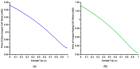
Figure 5.
Zero-coupon MECB price (a) and coupon-paying MECB price (b) for each .
Figure 5 shows that the Kendall tau correlation rates of trigger events are inversely proportional to zero-coupon and coupon-paying MECB prices. Rationally, it makes sense because if the value of the Kendall tau correlation rate of events is high, then the probability that the attachment points of the loss and fatality aggregates are exceeded is also high. This high probability causes investor interest in their involvement in MECBs to decline. This decline in investor interest occurs because they do not want to risk too significant a loss. So, the price also declines.
Next, we analyze the difference between the MECB price that involves and does not involve the correlation rate of events. By using the variable values at points (a), (b), (c), (d), (f), (g), (h), and (i) in Section 5.5, the difference between the MECB price that involves and does not involve the correlation rate of events for each tau is visually presented in Figure 6.
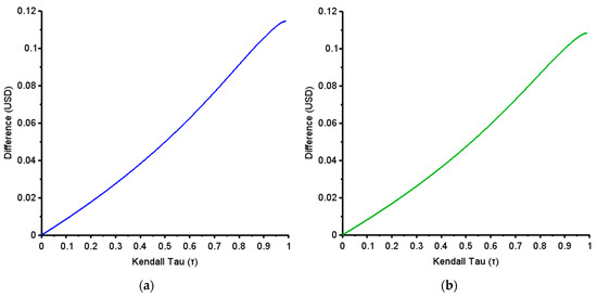
Figure 6.
The difference between the zero-coupon MECB prices that involve and do not involve the trigger event correlation rate for each (a) and the difference between the coupon-paying MECB prices that involve and do not involve the trigger event correlation rate for each (b).
Figure 6 shows that the difference between the zero-coupon MECB prices that involve and do not involve the correlation rate of events has a value in the interval USD. This interval is equivalent to the interval % of the principal . This is detrimental to investors because the price they pay for buying MECBs is higher even though it should be cheaper. The same thing also happened to the difference between coupon-paying MECB prices that involve and do not involve the trigger event correlation rate where the difference is in the interval USD or % of principal . The results of this analysis indicate that the correlation rate of events is essential to involve in MECB pricing.
6.2. The Effect of the Stochasticity of Inflation and Interest Rates on MECB Prices
This study considers the stochasticity of inflation and the interest rates in pricing MECB. In this subsection, we analyze its effect on MECB price. The analysis compares MECB prices that use constant and stochastic inflation and interest rates. The MECB prices that use a stochasticity of inflation and interest rates are the same in Section 5.5. In contrast, the MECB prices that use a constancy of inflation and interest rates were calculated using the inflation and interest rates in the United States in 2021. The comparison of MECB prices with constant and stochastic inflation and interest rates is presented in Table 5.
Table 5.
The comparison of MECB prices with constant and stochastic inflation and interest rates.
Table 5 shows that, in this case, MECB prices with a constancy of inflation and interest rates are higher than MECB prices with a stochasticity of inflation and interest rates. This can be detrimental to investors because the price they pay could have been lower. Thus, the involvement of stochastic assumptions on inflation and interest rates must be carried out in MECB pricing.
7. Conclusions
This study developed an MECB pricing model that involves trigger event correlation, inflation, and interest rates. The urgency of the involvement of the correlation rate of trigger events was so that the join-risk measurement of events can be carried out more fairly. Then, the inflation and interest rates were considered stochastically. The involvement of the stochasticity of inflation and interest rates was carried out so that the amount of return obtained by investors could be determined in real terms according to market fluctuations. The correlation rate of trigger events was accommodated using a copula, and the stochasticity of inflation and interest rates were simultaneously considered using an integrated autoregressive vector model.
The model simulation shows that the trigger events correlation rate has an inverse relationship with the MECB price. The higher the correlation rate of trigger events, the lower the MECB price and vice versa. This is rationally acceptable because the higher the correlation rate of trigger events, the higher the probability that these events will occur. It certainly causes investors’ interest in MECB to decline because the risk that they bear is too big. As a result, MECB prices are low. Then, if the correlation rate of trigger events is not considered in MECB pricing, the MECB price will be higher. This is detrimental to investors because they should be able to get a lower price. Finally, the simulation results show that the stochasticity of inflation and interest rates should be considered. This is obtained based on a significant MECB price difference where the MECB price that considers the stochasticity of the inflation and interest rates, is lower than the MECB price that does not consider it.
This research is expected to contribute to the development of an MECB pricing framework in postcatastrophe funding for countries around the world. This framework can produce a more reasonable estimate of MECB prices than the others because the factors involved in the calculation align with actual situations. Then, the effect of the correlation rate of trigger events and the stochasticity of the real interest rate on MECB prices can be used as a reference for investors in choosing MECBs. MECBs should have a low correlation and high real interest rates. Finally, for future research suggestions, the catastrophe risk status of a country might influence MECB prices. It can be assumed to be constant or nonconstant, but the nonconstant assumption is more described in real terms. Therefore, this can be a new research opportunity in the future.
Author Contributions
Conceptualization, S., I.G.P. and R.A.I.; methodology, M.P.A.S. and I.G.P.; software, Y.H. and I.G.P.; validation, S., R.A.I. and H.J.; formal analysis, R.A.I. and I.G.P.; investigation, S. and I.G.P.; resources, I.G.P.; data curation, N.B.A.H. and I.G.P.; writing—original draft preparation, R.A.I. and I.G.P.; writing—review and editing, S. and I.G.P.; visualization, R.A.I.; supervision, S., I.G.P. and H.J.; project administration, S. and I.G.P.; funding acquisition, S. and I.G.P. All authors have read and agreed to the published version of the manuscript.
Funding
This research was funded by the Directorate of Research, Community Service, and Innovation or DRPM Universitas Padjadjaran, grant number: 2064/UN6.3.1/PT.00/2022.
Institutional Review Board Statement
Not applicable.
Informed Consent Statement
Not applicable.
Data Availability Statement
Data are contained within the article.
Acknowledgments
Thanks to the Directorate of Research, Community Service, and Innovation or DRPM Universitas Padjadjaran. Thanks to Kemdikbudristek of the Republic of Indonesia for providing the Basic Research grant program. Thanks to the East Coast Environmental Research Institute (ESERI) Universiti Sultan Zainal Abidin, Malaysia; Research Center for Testing Technology and Standards, National Research and Innovation Agency, Indonesia; and Faculty of Science and Technology, Universiti Sains Islam Malaysia (USIM) for supporting this research collaboration.
Conflicts of Interest
The authors declare no conflict of interest.
Appendix A
Substitute with Equation (25).
is equivalent to Therefore, substitute with .
By using Equation (13), can substitute as follows:
Appendix B
Substitute with Equation (28).
is equivalent to Therefore, substitute with .
By using Equation (14), can substitute as follows:
References
- Coval, J.D.; Jurek, J.W.; Stafford, E. Economic catastrophe bonds. Am. Econ. Rev. 2009, 99, 628–666. Available online: http://www.jstor.org/stable/25592477 (accessed on 13 July 2022). [CrossRef]
- Jaimungal, S.; Chong, Y. Valuing clustering in catastrophe derivatives. Quant. Financ. 2013, 14, 259–270. [Google Scholar] [CrossRef]
- D’Arcy, S.P.; France, V.G. Catastrophe futures: A better hedge for insurers. J. Risk Insur. 1992, 59, 575–600. [Google Scholar] [CrossRef]
- Johnson, L. Catastrophe bonds and financial risk: Securing capital and rule through contingency. Geoforum 2013, 45, 30–40. [Google Scholar] [CrossRef]
- Cummins, J.D. CAT bonds and other risk-linked securities: State of the market and recent developments. Risk Manag. Insur. Rev. 2008, 11, 23–47. [Google Scholar] [CrossRef]
- Zeller, W. Securitization and Insurance: Characteristics of Hannover Re’s Approach. Geneva Pap. 2008, 33, 7–11. Available online: http://www.jstor.org/stable/41952967 (accessed on 15 July 2022). [CrossRef]
- Beer, S.; Braun, A.; Marugg, A. Pricing industry loss warranties in a Lévy–Frailty framework. Insur. Math. Econ. 2019, 89, 171–181. [Google Scholar] [CrossRef]
- Laster, D.; Raturi, M. What drives financial innovation in the insurance industry? J. Risk Financ. 2002, 3, 36–47. [Google Scholar] [CrossRef]
- Härdle, W.K.; Cabrera, B.L. Calibrating CAT bonds for Mexican earthquakes. J. Risk Insur. 2010, 77, 625–650. [Google Scholar] [CrossRef]
- Anggraeni, W.; Supian, S.; Sukono; Halim, N.B.A. Earthquake catastrophe bond pricing using extreme value theory: A mini-review approach. Mathematics 2022, 10, 4196. [Google Scholar] [CrossRef]
- Deng, G.; Liu, S.; Li, L.; Deng, C. Research on the pricing of global drought catastrophe bonds. Math. Probl. Eng. 2020, 2020, 3898191. [Google Scholar] [CrossRef]
- Sukono; Juahir, H.; Ibrahim, R.A.; Saputra, M.P.A.; Hidayat, Y.; Prihanto, I.G. Application of compound Poisson process in pricing catastrophe bonds: A systematic literature review. Mathematics 2022, 10, 2668. [Google Scholar] [CrossRef]
- Woo, G. Territorial diversification of catastrophe bonds. J. Risk Financ. 2001, 2, 39–45. [Google Scholar] [CrossRef]
- Organization for Economic Cooperation and Development (OECD). Terrorism Risk Insurance in OECD Countries; Policy Issues in Insurance; OECD Publishing: Paris, France, 2005. [Google Scholar] [CrossRef]
- Woo, G. A catastrophe bond niche: Multiple event risk. In Proceedings of the NBER Insurance Workshop, Cambridge, UK, 6–7 February 2004. [Google Scholar]
- Reshetar, G. Pricing of Multiple-Event Coupon Paying CAT Bond; Working Paper; Swiss Banking Institute: Zürich, Switzerland, 2008. [Google Scholar]
- Ling, T.; Tianyuan, L.; Fei, Z. The pricing of catastrophe bond by Monte Carlo simulation. In Proceedings of the International Conference on Risk Management and Engineering Management, Beijing, China, 4–6 November 2008. [Google Scholar]
- Sun, L.; Turvey, C.G.; Jarrow, R.A. Designing catastrophic bonds for catastrophic risks in agriculture: Macro hedging long and short rains in Kenya. Agric. Financ. Rev. 2015, 75, 47–62. [Google Scholar] [CrossRef]
- Chao, W.; Zou, H. Multiple-event catastrophe bond pricing based on CIR-Copula-POT model. Discret. Dyn. Nat. Soc. 2018, 2018, 5068480. [Google Scholar] [CrossRef]
- Ibrahim, R.A.; Sukono; Napitupulu, H.N. Multiple-trigger catastrophe bond pricing model and its simulation using numerical methods. Mathematics 2022, 10, 1363. [Google Scholar] [CrossRef]
- Wei, L.; Liu, L.; Hou, J. Pricing hybrid-triggered catastrophe bonds based on copula-EVT model. Quant. Financ. Econ. 2022, 6, 223–243. [Google Scholar] [CrossRef]
- Jarrow, R.A. A simple robust model for CAT bond valuation. Financ. Res. Lett. 2010, 7, 72–79. [Google Scholar] [CrossRef]
- Groenewold, N. The adjustment of the real interest rate to inflation. Appl. Econ. 1989, 21, 947–956. [Google Scholar] [CrossRef]
- Carmichael, J.; Stebbing, P.W. Fisher’s paradox and the theory of interest. Am. Econ. Rev. 1983, 73, 619–630. Available online: https://www.jstor.org/stable/1816562 (accessed on 4 September 2022).
- Zimbidis, A.A.; Frangos, N.E.; Pantelous, A.A. Modeling earthquake risk via extreme value theory and pricing the respective catastrophe bonds. ASTIN Bull. 2007, 37, 163–183. [Google Scholar] [CrossRef][Green Version]
- Nowak, P.; Romaniuk, M. Pricing and simulations of catastrophe bonds. Insur. Math. Econ. 2012, 52, 18–28. [Google Scholar] [CrossRef]
- Nowak, P.; Romaniuk, M. Valuing catastrophe bonds involving correlation and CIR interest rate model. Comput. Appl. Math. 2018, 37, 365–394. [Google Scholar] [CrossRef]
- Liu, J.; Xiao, J.; Yan, L.; Wen, F. Valuing catastrophe bond involving credit risks. Math. Probl. Eng. 2014, 2014, 563086. [Google Scholar] [CrossRef]
- Ma, Z.G.; Ma, C.Q. Pricing catastrophe risk bonds: A mixed approximation method. Insur. Math. Econ. 2013, 52, 243–254. [Google Scholar] [CrossRef]
- Chaubey, Y.P.; Garrido, J.; Trudeau, S. On the computation of aggregate claims distributions: Some new approximations. Insur. Math. Econ. 1998, 23, 215–230. [Google Scholar] [CrossRef]
- Tang, Q.; Yuan, Z. CAT bond pricing under a product probability measure with POT risk characterization. ASTIN Bull. 2019, 49, 457–490. [Google Scholar] [CrossRef]
- Ma, Z.; Ma, C.; Xiao, S. Pricing zero-coupon catastrophe bonds using EVT with doubly stochastic Poisson arrivals. Discret. Dyn. Nat. Soc. 2017, 2017, 3279647. [Google Scholar] [CrossRef]
- Burnecki, K.; Kukla, G.; Taylor, D. Pricing catastrophe bonds. In Statistical Tools for Finance and Insurance, 2nd ed.; Cizek, P., Härdle, W., Weron, R., Eds.; Springer: Berlin, Germany, 2005; pp. 97–114. [Google Scholar] [CrossRef]
- Cummins, J.D.; Weiss, M.A. Convergence of insurance and financial markets: Hybrid and securitized risk-transfer solutions. J. Risk Insur. 2009, 76, 493–545. [Google Scholar] [CrossRef]
- Loubergé, H.; Kellezi, E.; Gilli, M. Using catastrophe-linked securities to diversity insurance risk: A financial analysis of CAT bonds. J. Insur. Issues 1999, 22, 125–146. [Google Scholar]
- Dickson, D.C.M. Insurance Risk and Ruin; Cambridge University Press: Cambridge, UK, 2005; pp. 83–89. [Google Scholar]
- Klugman, S.A.; Panjer, H.H.; Willmot, G.E. Loss Models: From Data to Decisions, 4th ed.; John Wiley & Sons: Hoboken, NJ, USA, 2019; pp. 151–157. [Google Scholar]
- Salvadori, G.; Michele, C.D.; Kottegoda, N.T.; Rosso, R. Extremes in Nature: An Approach Using Copulas; Springer: Dordrecht, The Netherlands, 2007; pp. 131–141. [Google Scholar]
- Ross, S.M. Stochastic Processes, 2nd ed.; John Wiley & Sons: Hoboken, NJ, USA, 1996; pp. 98–100. [Google Scholar]
- Li, J.; Balasooriya, U.; Liu, J. Using hierarchical Archimedean copulas for modelling mortality dependence and pricing mortality-linked securities. Ann. Actuar. Sci. 2021, 15, 505–518. [Google Scholar] [CrossRef]
- Hasebe, T. Copula-based maximum-likelihood estimation of sample-selection models. Stata J. 2013, 13, 547–573. [Google Scholar] [CrossRef]
- Dhaene, J. Stochastic interest rates and autoregressive integrated moving average processes. ASTIN Bull. 1989, 19, 43–50. [Google Scholar] [CrossRef][Green Version]
- Kierzkowski, H. A Generalization of the Fisher Equation. Econ. Rec. 1979, 55, 261–266. [Google Scholar] [CrossRef]
- Kyereme, S.S. Exchange rate, price, and output interrelationships in Ghana: Evidence from vector autoregressions. Appl. Econ. 1991, 23, 1801–1810. [Google Scholar] [CrossRef]
- Ruch, F.; Balcilar, M.; Gupta, R.; Modise, M.P. Forecasting core inflation: The case of South Africa. Appl. Econ. 2020, 52, 3004–3022. [Google Scholar] [CrossRef]
- Wei, W.W.S. Time Series Analysis: Univariate and Multivariate Methods, 2nd ed.; Pearson Addison Wesley: White Plains, NY, USA, 2006; pp. 384–386. [Google Scholar]
- Nagler, T.; Schepsmeier, U.; Stoeber, J.; Brechmann, E.C.; Graeler, B.; Erhardt, T.; Almeida, C.; Min, A.; Czado, C.; Hofmann, M.; et al. Package ‘VineCopula’. Available online: https://cran.r-project.org/web/packages/VineCopula/VineCopula.pdf (accessed on 16 June 2022).
- Trapletti, A.; Hornik, K.; LeBaron, B. Package ‘Tseries’. Available online: https://cran.r-project.org/web/packages/tseries/tseries.pdf (accessed on 16 June 2022).
- Tsay, R.S. Package ‘MTS’. Available online: https://cran.r-project.org/web/packages/MTS/MTS.pdf (accessed on 16 June 2022).
- Tsay, R.S. Multivariate Time Series Analysis with R and Financial Application; John Wiley & Sons: Hoboken, NJ, USA, 2014; pp. 63–64. [Google Scholar]
- Kocherlakota, N.R. Stabilization with fiscal policy. J. Monet. Econ. 2022, 131, 1–14. [Google Scholar] [CrossRef]
- Nuel, G. Cumulative distribution function of a geometric Poisson distribution. J. Stat. Comput. Simul. 2008, 78, 385–394. [Google Scholar] [CrossRef]
Publisher’s Note: MDPI stays neutral with regard to jurisdictional claims in published maps and institutional affiliations. |
© 2022 by the authors. Licensee MDPI, Basel, Switzerland. This article is an open access article distributed under the terms and conditions of the Creative Commons Attribution (CC BY) license (https://creativecommons.org/licenses/by/4.0/).