Article

An Inventory Model in a Three-Echelon Supply Chain for Growing Items with Imperfect Quality, Mortality, and Shortages under Carbon Emissions When the Demand Is Price Sensitive

by
Cynthia Griselle De-la-Cruz-Márquez
1,
Leopoldo Eduardo Cárdenas-Barrón
1,*,
Buddhadev Mandal
2,
Neale R. Smith
1,
Rafael Ernesto Bourguet-Díaz
1,
Imelda de Jesús Loera-Hernández
1,
Armando Céspedes-Mota
1 and
Gerardo Treviño-Garza
1
1
Tecnologico de Monterrey, School of Engineering and Sciences, Ave. Eugenio Garza Sada 2501, Monterrey 64849, NL, Mexico
2
Regent Education and Research Foundation, Barrackpore, Kolkata 700121, India
*
Author to whom correspondence should be addressed.
Mathematics 2022, 10(24), 4684; https://doi.org/10.3390/math10244684
Submission received: 12 October 2022 / Revised: 25 November 2022 / Accepted: 27 November 2022 / Published: 10 December 2022

Abstract

:
This research develops an optimization model for growing items in a supply chain with three stages: farmer, processor, and retailer while considering imperfect quality, mortality, shortages with full backordering, and carbon emissions. In the farmer stage, during the growing period, not all articles survive until the end of the period, so a density function of the probability of survival and death of the growing articles is taken into account. Moreover, it is considered imperfect quality in the retailer’s stage because as the supply chain goes down, there exists a greater probability of product defects. Here, the end customer (consumer) can detect poor-quality aspects such as poorly cut, poorly packed, expired products, etc. An inventory model that maximizes the expected total profit is formulated for a single type of growing items with price-dependent polynomial demand. An algorithm is developed to solve the optimization problem generating the optimal solution for order quantity, backordering quantity, selling price, and the number of shipments that maximizes the expected total profit per unit of time, and a numerical example is used to describe the applicability of the proposed inventory model. Finally, a sensitivity analysis has been carried out for all the input parameters of the inventory model, where the effect of each of the parameters on the decision variables is shown to extract some management knowledge. It was found that holding costs in the three stages of the supply chain have a substantial impact on the total profit per unit of time. In addition, as the demand scale parameter increases, the company must raise the selling price, which directly impacts the expected total profit per unit of time. This inventory model has the advantage that it can be applied to any growing item, including animals or plants, so it helps the owners of farms or crops to generate the most significant possible profit with their existing resources.

1. Introduction

Inventory management helps organizations to determine how much stock to purchase and at what time in order to have always enough inventories to cover the demand of the consumers. In the inventory theory field, many inventory models are available; the most famous model is the economic order quantity (EOQ) inventory model. Here, a brief literature review related to economic order quantity (EOQ) inventory models is presented. Specifically, the literature review is structured in the following areas: inventory models for growing items, inventory models with carbon emissions, inventory models with imperfect quality, inventory models with shortages, and inventory models with price-dependent demand. Internally in each area, the review is given chronologically, starting from the first work to the most recent.

1.1. EOQ Inventory Models for Growing Items

Unlike manufacturing products, there are certain goods called growing items, and as the name implies, they grow during the storage period, and these are all types of animals. It is important to remark that there are two types of growing items those that are seasonal and those that are sold all year round. Most of the animals sold in the western world are present all year round, such as cattle, chickens, pigs, ducks, sheep, buffalo, turkeys, wild boars, ostriches, and rabbits. The animals usually sold in certain seasons are commonly marine ones such as tuna, shrimp, crab, lobster, oysters, and some types of fish such as trout, cod, among others.
It was noted that there is a lack of research in the area of inventory management for growing items. However, recently the growing items are receiving attention in inventory management research. This type of item is an essential part of daily life as most serve as food in some supply chains, so having a better understanding of this kind of item enriches the knowledge in this new and significant field of inventory theory. The first time that a new class of inventory model for growing items was proposed by Rezaei [1]. The inventory models for growing items have been attracting researchers and academicians worldwide since 2014. Figure 1 shows the evolution of inventory models for growing items over time from 2014 to 2022. Rezaei [1] presented a general mathematical model for any of growing items and then for a specific type of poultry. Later, Ritha and Haripriya [2] proposed a mathematical model with shortages for growing items aimed at poultry products. Afterward Zhang et al. [3] studied the inventory management problems of growing items and developed an inventory model with this category of items considering carbon emissions. Subsequently, Dhanam and Jesintha [4] formulated a fuzzy inventory model for slow- and fast-growing items with deterioration in a single period, considering that the demand rate is random and the deterioration rate is constant. Next, Sebatjane [5] built three inventory models for growing items contemplating imperfect quality, two growing and storage facilities, and incremental quantity discounts. After that, Nobil et al. [6] introduced an economic order quantity (EOQ) inventory model for growing items. They examined an inventory system of poultries in which newborn items are fed to reach the ideal weight for consumers. The inventory model assumes that shortage is permitted, so consumers must wait for fresh items.
Sebatjane and Adetunji [7] derived an inventory system where ordered items grow during the inventory cycle and in which a fraction of the items is of lower quality than desired by maximizing the total expected profit. That same year, Sebatjane and Adetunji [8] created an inventory model for growing items in which the supplier of the items offered a scheme of incremental quantity discounts. In a subsequent paper, Sebatjane and Adetunji [9] devised a coordinated inventory control model for growing items for a supply chain with farming, processing, and retail operations. For the first time, Khalilpourazari and Pasandideh [10] presented a new mathematical model for multi-item economic order quantity for growing items considering various operational constraints. They considered different operational restrictions to propose a realistic inventory model, including an on-hand budget, warehouse capacity, and total allowable holding cost constraints. To provide an appropriate mathematical inventory model for ameliorating and deteriorating items, Malekitabar et al. [11] suggested an inventory model for products called growing-mortal items in a two-echelon supply chain consisting of one supplier and one farmer. Later, Nobil and Taleizadeh [12] produced an EOQ inventory model for growing items by assuming that items grow with a function that has a linear approximation. Then, Eveline and Ritha [13] purported an EOQ inventory model for growing items (poultries), and they investigated the various costs of the system. It is presumed that shortages are permitted and are completely backlogged. Garza-Cabello [14] developed an inventory model with planned shortages for growing items with imperfect quality. The inventory model is extended to three different models, which vary among them in the cost of feeding because each inventory model represents a different situation of growth of the items. Sebatjane and Adetunji [15] continued working on developing an inventory model with growing items. This time, they recommended an inventory model for managing stock in a three-tier perishable food supply chain comprised of the growing stage, processing phase, and retailing to maximize profits for the joint supply chain. In subsequent research work, Sebatjane y Adetunji [16] established an integrated inventory control model for a four-echelon supply chain which involved the following levels: farming, processing, screening, and retailer. Gharaei and Almehdawe [17] provided new inventory models focusing on growing items from agricultural industries such as fishing, poultry, and livestock. They considered in their economic growing quantity (EGQ) inventory model the density functions of survival probability and mortality of a growing item since several items have material changes during a planning period, such as amelioration, deterioration, and growth. Hidayat et al. [18] prepared a new mathematical model for growing items that relax three implicit assumptions of the classical EOQ: the ordered items do not increase, their unlimited capacity, and a total budget. Mokhtari et al. [19] generated a class of production-inventory models related to the livestock growing process, where livestock grows during the growing period. Additionally, the slaughtered livestock may deteriorate during the sales period. Nishanthi [20] addressed an inventory model for growing items with imperfect quality, shortages with fully backordered, and proper disposal of animal mortality during their growth period. Pourmohammad Zia and Karimi [21] discussed optimal management policies for inventories with growing items where the quality degradation of these items is modeled as deterioration. Afzal and Alfares [22] extended inventory models for growing items by considering quality inspections, permissible shortages with complete backordering, and holding costs during both growth and consumption periods. Sebatjane [23] made six inventory models for growing items. Sebatjane and Adetunji [24] introduced an integrated model for inventory control in a three-tier supply chain for growing items. Alfares and Afzal [25] proposed an inventory model for growing items that considers quality, allowable shortages with full backordering, and holding costs during both growth and consumption periods. Mittal and Sharma [26] developed an inventory model for growing items to determine the optimal order quantity of items to order at the beginning of a cycle, the optimal length of the growing process, and the optimal total profit for the retailer in the presence of a deferral allowed in payments. Luluah et al. [27] formulated an optimization model of order quantities for growing items by considering incremental discounts and imperfect quality. Gharaei and Almehdawe [28] designed and optimized a sustainable inventory model for growing items that evaluate the environmental effects of Greenhouse Gases (GHGs) emitted from produced manure, fermentation processes, and transportation, as well as their cost concerning carbon tax. Mahato et al. [29] investigated an inventory model for growing items for a two-echelon supply chain with a hybrid-price-stock-dependent demand under a trade credit policy. De-la-Cruz-Márquez et al. [30] explored an inventory model for growing items with poor quality when the demand is price sensitive under carbon emissions and shortages. Maity et al. [31] analyzed an economic order quantity inventory model for fisheries production. They assumed that the growth rate is a linear function. Pourmohammad-Zia et al. [32] examined dynamic pricing and inventory control policies in a two-level food supply chain of growing and deteriorating inventory that involves a rearing farm comprised of a supplier and a retailer. In a successive paper, Pourmohammad-Zia et al. [33] addressed an inventory model in a three-level that embraces growing items such as poultry and livestock. The chain involves a breeding farm as a supplier, a processed food producer as a manufacturer, and multiple processed food retailers. Rana et al. [34] researched the effect of carbon emissions from the poultry industry and formed an inventory model with shortages with partial backlogging. Choudhury and Mahata [35] considered a two-echelon sustainable supply chain model for growing items with a supplier–retailer scenario to reduce carbon emissions. Pourmohammad-Zia [36] reviewed in detail the investigations related to growing items to provide the researchers with clear insights into the structure of the current literature, its main gaps, and promising directions for future research. Sharma and Saraswat [37] developed a mathematical model for growing items by considering various operational constraints. That same year, Saraswat and Sharma [38] formulated an inventory model for growing items with price-dependent demand, mortality, and deterioration, where shortages are partially backlogged. They optimized the total cost by determining the optimal ordered quantity and total cycle length. Sitanggang et al. [39] developed an optimization model to select the order quantity of growing items by taking into account imperfect quality and incremental discount, involving three members of the supply chain: farmers, processors, and retailers.
Faraudo Pijuan [40] made an inventory model to optimize the products’ inventory cycle and price, adapting it to the needs of the agricultural and livestock industry so that the products can grow, emit CO2 emissions and be of imperfect quality. Sebatjane and Adetunji [41] built a model for managing inventory in a three-echelon supply chain for growing items with distinct farming, processing, and retail operations under the assumption that the inventory has a specified expiration date. Sebatjane [42] proposed an inventory management strategy for a multi-echelon perishable food supply chain with growing and deteriorating items. This integrated inventory model optimizes the performance of the entire food supply chain with the impact of preservation technologies due to the perishable nature of food products. Abbasi et al. [43] optimized an EOQ inventory model, including products that can grow during replenishment, such as livestock. In addition, they assumed that the system’s products have a stochastic demand and that a specific part of them has a lower desired quality. Sharma and Mittal [44] analyzed an inventory model for growing items with trade credit that maximizes the total profit. Sharma and Saraswat [45] formulated two inventory models for the growing items under realistic aspects such as mortality and deterioration. One proposed inventory model considers permissible delay in payment, and another does not consider this. Table 1 provides a general overview of the inventory models for growing items available in the literature. To sum up, the majority fails to consider jointly the price-dependent demand, shortages, imperfect quality, mortality, carbon emissions, and supply chain with three stages.

1.2. EOQ Inventory Models with Carbon Emissions

Today the concern for the environment has increased significantly, and it seeks to develop inventory systems that reduce carbon emissions. For instance, Huang et al. [46] investigated the effects of carbon policies and green technologies on the integrated inventory of a two-echelon supply chain with consideration of carbon emissions during product production, transportation, and storage. Yu et al. [47] studied an inventory optimization problem involving perishable products under a carbon policy. Utama et al. [48] derived the sustainable economic order quantity (SEOQ) model that considers transportation, warehouse costs, emission of carbon, and capacity. Yadav and Khanna [49] dealt with an inventory model for perishable products with an expiration date under the carbon tax policy to achieve sustainability goals. Hasan et al. [50] proposed three models to optimize the inventory level and technology investment under a carbon tax, cap-and-trade, and strict carbon limit regulations. De et al. [51] explored carbon emission issues over the production system within the context of joint inventory control and sustainable trade credit financing for deteriorating items in a supplier–retailer–customer model under the volumetric fuzzy system. Mashud et al. [52] recommended a sustainable price-dependent demand inventory model with controllable carbon emissions to reduce the CO2 emissions from farm warehousing activity. Zhang et al. [53] studied the impacts of cap-and-trade regulation on a three-echelon closed-loop supply chain network, revealing that, in some cases, there is a consistency between the carbon emission reduction target of the government and the profit target of enterprises. Bhattacharjee and Sen [54] formulated an inventory model to study the earnings made by the supplier when the product has a price and stock-dependent demand and examine the effect of carbon emission and shelf-life. Gautam et al. [55] constructed an inventory model to handle defective products by considering energy usage during production and the cost of carbon emissions. Currently, many studies take into consideration that companies’ carbon emissions come from all operations. For example, Chen et al. [56] considered carbon emissions related to ordering, inventory holding, and purchasing. In addition, Zhang et al. [3] said that growing items such as poultry, livestock, among others, produce carbon emissions in transport, inventory, growing stage of the process from purchase to sale, and they considered the emissions associated with initiating orders, inventory holding, feeding, and purchasing. Mishra et al. [57], in the same way, consider the carbon emissions for all the operations of their inventory model. Under this same direction, in each stage of the proposed inventory model, there are several operations. This research work assumes that in each stage carbon emissions are emitted, except in shortages period, since when these occur at the beginning, these do not physically exist but are only registered in some database indicating that these have to be replaced until the next cycle. Obviously, the shortages will emit emissions once these become a product that is sold. Furthermore, in the literature review, it is found that implementing a carbon tax policy to control the carbon emissions of a supply chain is adequate.
Gases that trap heat in the atmosphere are called greenhouse gases. According to the United States Environmental Protection Agency (EPA) [58] the highest concentration in the world is carbon dioxide, C O 2 , which enters the atmosphere through burning fossil fuels (coal, natural gas, and oil), solid waste, trees, and various animals. In second place is Methane, C H 4 ; methane emissions are generated in livestock and other agricultural practices. Finally, the nitrous oxide, N 2 O , emitted during agricultural and industrial activities. Moreover, De Boer et al. [59] mention that livestock production is recognized to contribute significantly to the emission of greenhouse gases, mainly through the emission of carbon dioxide, methane, and nitrous oxide. Therefore, this research work only considers carbon emissions since these are the gases emitted most by growing items; however, the proposed inventory model can consider other type of greenhouse gases.

1.3. EOQ Inventory Models with Imperfect Quality

Although any industry produces a certain percentage of defective items, all organizations want to produce good quality items for their customers. That is why imperfect quality has been a relevant feature to consider within systems and inventories. For example, Nobil et al. [60] calculated the optimal reorder point for Salameh and Jaber [61] ’s inventory model, which is a critical milestone for managers to determine the appropriate timing of the order. Daryanto et al. [62] presented a retailer’s inventory model considering an imperfect production process and material handling that cause some defective items, where the faulty items possess a fraction of their original utility. Sepehri et al. [63] elaborated a sustainable production-inventory model for poor quality deteriorating items, where items deteriorate at a constant rate and the deterioration progress is controlled by investing in preservation technology. Cárdenas-Barrón et al. [64] introduced an economic order quantity (EOQ) inventory model for imperfect and perfect quality items by considering that the imperfect ones are sent as a single lot to a repair shop for reworking. Kishore et al. [65] proposed an inventory model with a tri-tier supply chain (manufacturer–wholesaler–retailer), where the consignment received is unreliable due to defective items.

1.4. EOQ Inventory Models with Shortages

Within the various inventory systems that have been developed over time, those that consider a policy with shortages have proven to be better than those that do not view this policy because there is a lower cost of storage, and customers still maintain fidelity. Mashud [66] created a deteriorating EOQ inventory model according to consideration of the price- and stock-dependent demand and fully backlogged shortages. Öztürk [67] built a deterministic production-inventory model with defective items, an imperfect rework process, and shortages backordered. Mahato and Mahata [68] studied a green economic order quantity model with capacity constraints under order-size-dependent trade credit and all-units discount along with minimizing carbon for a cleaner environment. In addition, shortages are allowed with partial backordering. Iswarya and Karpagavalli [69] considered a fuzzy inventory model with shortages. Mallick et al. [70] introduced a supplier-retailer supply chain system for perishable goods under fuzzy lead time and fully backlogged shortages.

1.5. EOQ Inventory Models with Price Dependent Demand

Some of the most common assumptions in studying economic order quantity (EOQ) inventory models are to consider a constant demand rate independent of the unit selling price. Nevertheless, in many real-world situations, the demand rate is not constant and may be price-dependent, which must be allowed in the inventory model. The polynomial price-dependent demand is selected due to the fact that this type of demand function models the price well; in addition, this polynomial price-dependent demand contains, as a special case, a demand that is widely used in the literature, which is linear price-dependent demand. Some inventory systems with price-dependent demand are available in the literature. Several of these studies assume a pricing optimization problem with a deterministic demand that is a linear function of price. Malekitabar et al. [11] developed an inventory model for growing items with the selling price to the farmer, which is a linear descending function of item weight. San-Jose et al. [71] studied a lot-size inventory problem for products whose demand patterns depend on price, advertising frequency, and time using a polynomial function. Singer and Khmelnitsky [72] developed an inventory model to establish the optimal price for a product where the demand is price-sensitive. Later, Miah et al. [73] suggested a model considering a cost, time, and stock-dependent realistic demand function with two modes of discount policy. Ruidas et al. [74] purported an imperfect production inventory model under various regulatory carbon emission policies. The demand for the product is assumed to be a linearly decreasing function of the product’s sale price. Pando et al. [75] considered an inventory model where the demand rate depends on the selling price and the stock level. Wang and Wan [76] analyzed a bi-objective mixed-integer mathematical model considering customer demands price- and greenness-sensitive for the case of multiple products. Feng et al. [77] explored an inventory system: the demand curve depends on unit price, displayed volume, and sell-by date, and the supplier and the retailer agree with an advance-cash-credit (ACC) payment scheme. Recently, Macías-López et al. [78] developed an inventory model for perishable items, where the demand for perishable items is a multivariate function of price, current stock quantity, and freshness condition. For the price, six different price-dependent demand functions are used: linear, isoelastic, exponential, logit, logarithmic, and polynomial.
To the authors’ knowledge, no published model is developing the optimal policy for an inventory model in a three-echelon supply chain for growing items with price-dependent polynomial demand, considering mortality, imperfect quality, shortages with full backordering, and carbon emissions. The remainder of the paper is organized as follows. Section 2 presents the inventory model notation. Section 3 states the assumptions of the inventory model. Section 4 shows the development of the inventory model and the formulation of the optimization problem. Section 5 derives the theoretical results and constructs an algorithm to solve the inventory problem optimally. Section 6 solves a numerical example to illustrate the procedure for solving the inventory problem. Section 7 provides a sensitivity analysis of input parameters to gain managerial insights. Finally, Section 8 gives some conclusions about the research work and future research areas.

2. Notation

The following notation is used throughout the paper to formulate the three-echelon supply chain inventory model for growing items with imperfect quality, carbon emissions, and shortages:
Parameters:
Selling prices:
p f Farmer’s selling price (Processor’s purchasing cost) per weight unit of live items (currency symbol/unit of weight)
p p Processor’s selling price (Retailer’s purchasing cost) per weight unit of lot size (currency symbol/unit of weight)
p v Retailer’s selling price of imperfect items (currency symbol/unit of weight)
Revenues:
T R f Farmer’s total revenue (currency symbol/period)
T R p Processor’s total revenue (currency symbol/period)
T R r Retailer’s total revenue (currency symbol/period)
Costs:
p Farmer’s purchasing cost (currency symbol/unit of weight)
K f Farmer’s setup cost (currency symbol/cycle)
K p Processor’s setup cost (currency symbol/cycle)
K r Retailer’s ordering cost (currency symbol/cycle)
c f Farmer’s feeding cost (currency symbol/unit of weight)
m f Farmer’s mortality cost (currency symbol/unit of weight)
h l Farmer’s holding cost of the growing live items (currency symbol/unit of weight/unit of time)
h s Processor’s holding cost of the slaughtered items (currency symbol/unit of weight/unit of time)
h r Retailer’s holding cost of processed items (currency symbol/unit of weight/unit of time)
p c Processor’s processing cost (currency symbol/unit of weight/unit of time)
z Retailer’s inspection cost (currency symbol/unit of weight)
b Retailer’s shortage cost (currency symbol/unit of weight/unit of time)
Carbon
emission
costs:
θ Carbon tax rate (currency symbol/amount of carbon emissions)
E c f Farmer’s carbon emissions cost (currency symbol)
E c p Processor’s carbon emissions cost (currency symbol)
E c r Retailer’s carbon emissions cost (currency symbol)
p Amount of carbon emissions produced during farmer’s purchasing activity (unit of weight/unit of time)
p f Amount of carbon emissions generated during processor’s purchasing activity (unit of weight/unit of time)
p p Amount of carbon emissions made during retailer’s purchasing activity (unit of weight/unit of time)
K f Amount of carbon emissions produced during farmer’s setup process (unit of weight/unit of time)
K p Amount of carbon emissions caused during processor’s setup process (unit of weight/unit of time)
K r Amount of carbon emissions created during retailer’s ordering process (unit of weight/unit of time)
c f Amount of carbon emissions originated during farmer’s feeding period (unit of weight/unit of time)
m f Amount of carbon emissions delivered during farmer’s mortality process (unit of weight/unit of time)
h l Amount of carbon emissions made by farmer’s holding of live items in warehouse (unit of weight/unit of time)
h s Amount of carbon emissions produced by processor’s holding of the slaughtered items in warehouse (unit of weight/unit of time)
h r Amount of carbon emissions caused by retailer’s holding items in warehouse (unit of weight/unit of time)
p c Amount of carbon emissions created during processor’s period (unit of weight/unit of time)
Z Amount of carbon emissions originated during retailer´s inspection process (unit of weight/unit of time)
π Scale parameter for the price dependent demand
ρ Sensitivity parameter for the price dependent demand
u Demand power index
r Inspection rate (unit of weight/unit of time)
P Processing rate (unit of weight/unit of time)
a 
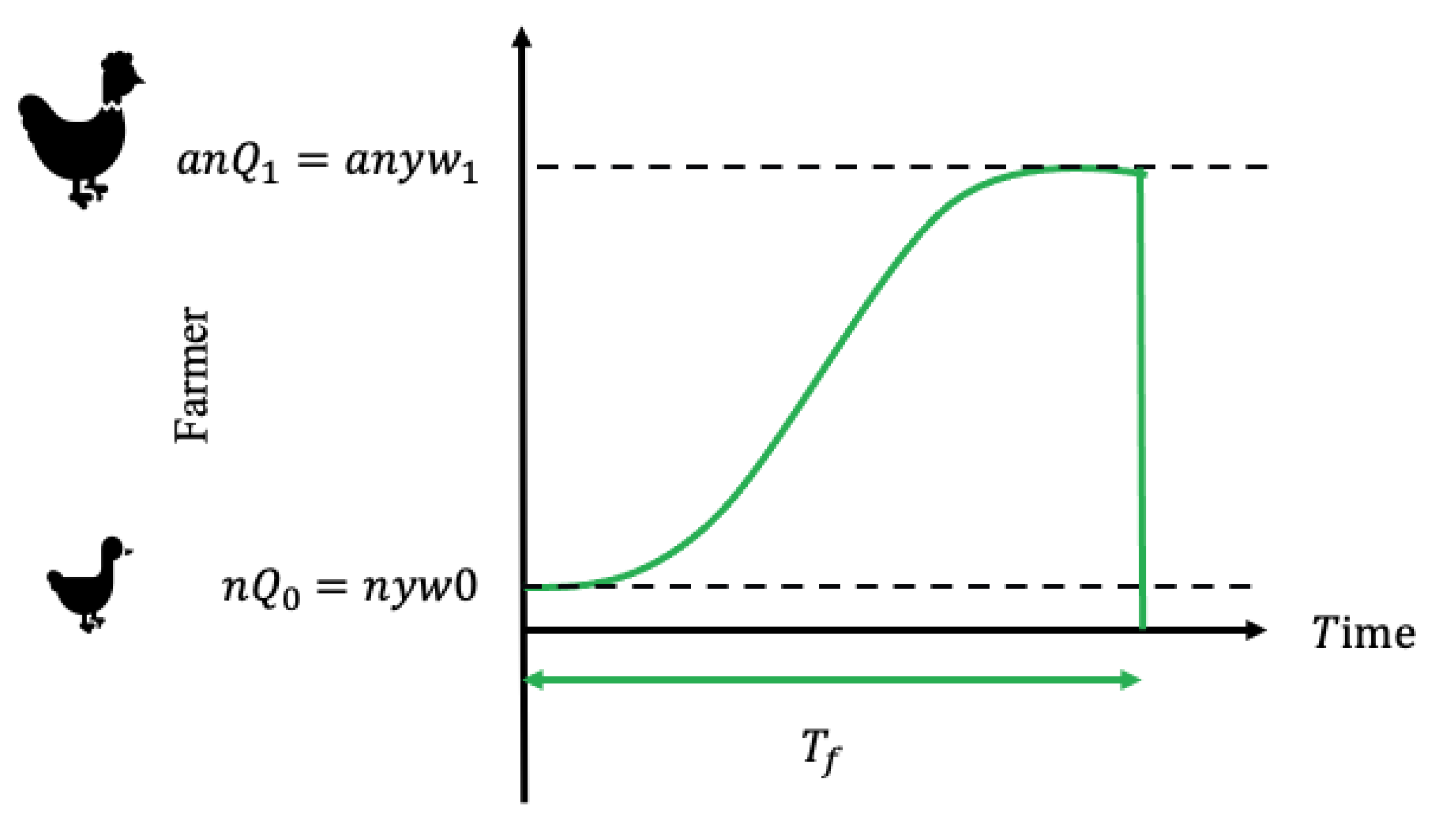
Fraction of the live items that survive throughout the growth period
E [ a ] Expected value of the percentage of the live items that survive throughout the growth period
1 E [ a ] Expected value of the percentage of the dead items which die during the growth period
α Asymptotic weight of each item (unit of weight)
β Integration constant (numeric value)
λ Growth rate (numeric value/unit of time)
Percentage of slaughtered items that are of imperfect quality
( 0 x 1 )
x Percentage   of   slaughtered   items   that   are   of   imperfect   quality   ( 0 x 1 )
E [ x ] Expected   value   of   the   percentage   of   imperfect   items   ( 0 E [ x ] 1 )
1 E [ x ] Expected   value   of   the   percentage   of   perfect   items   ( 0 1 E [ x ] 1 )
w 0 Weight of a newborn item (unit of weight)
w 1 Target weight of a grown item (unit of weight)
w t Weight of an item at time t (unit of weight)
T f Duration of farmer’s growth period (unit of time)
T p Processor s   cycle   time   T p = n T (unit of time)
t 1 Inspection period to complete B units of weight of perfect quality (unit of time)
t 2 Inspection   period   for   remaining   units   of   weight   of   the   lot ,   y w 1 D t 1 B (unit of time)
t 3 Consumption period of perfect items after inspection time (unit of time)
t 4 Shortages accumulation period (unit of time)
Decision
variables:
y Farmer’s order quantity of newborn items (units)
B Backordering quantity (unit of weight)
p r Retailer´s selling price of perfect items (currency symbol/unit of weight)
n 
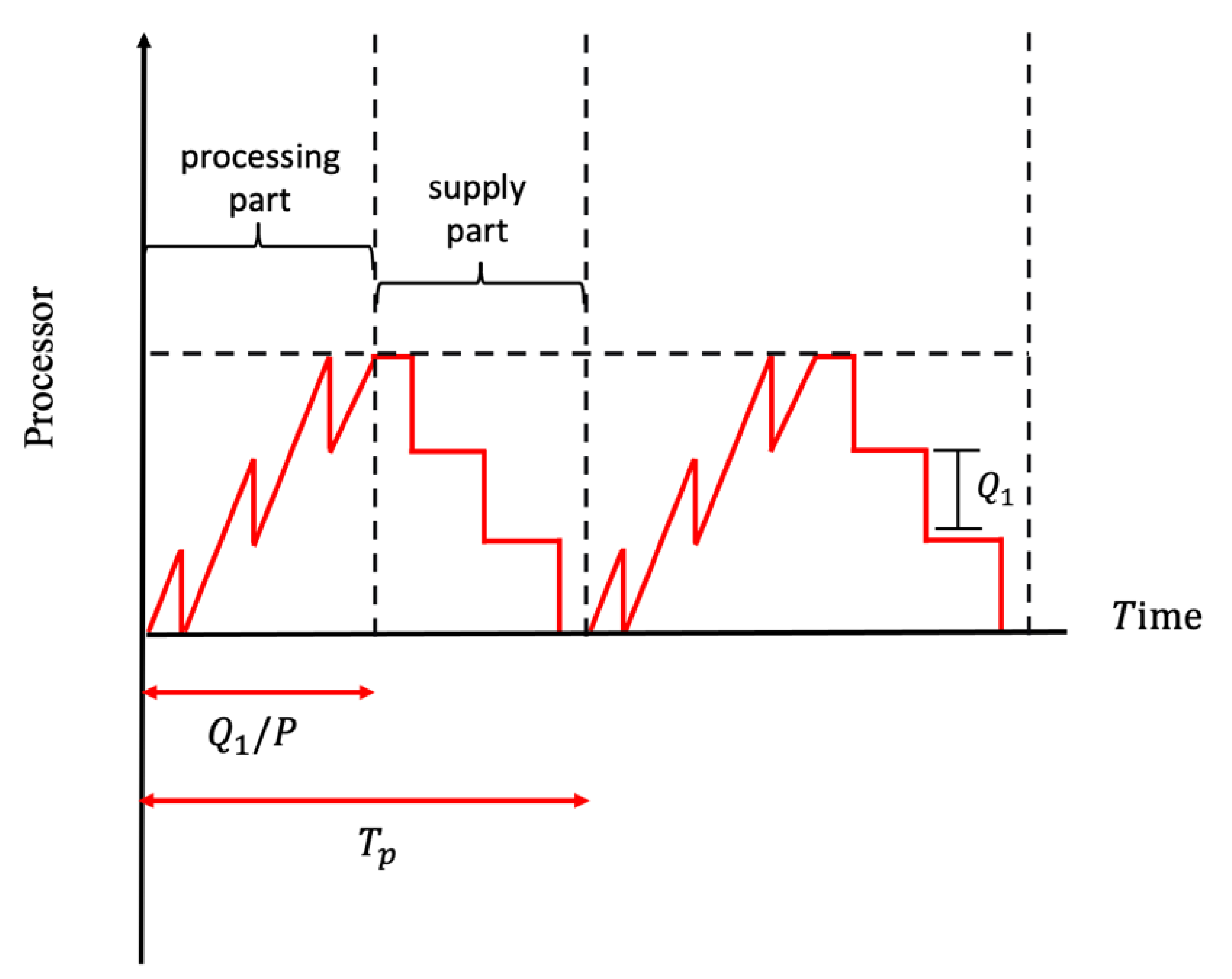
Number of shipments from the processor to the retailer per unit period of the processor
Decision dependent variables:
T Retailer’s cycle time (unit of time)
Q 0 Total weight at the beginning of farmer’s growth period, Q 0 = y w 0 (unit of weight)
Q 1 Total weight of the retailer’s lot size per shipment Q 1 = y w 1 (unit of weight)
y f Farmer s   order   quantity   of   newborn   items   per   period   y f = n y
Functions:
D ( s ) Price dependent demand function (unit of weight/unit of time)
w t ( t ) Growth function
g ( x ) Probability density function of the percentage of imperfect items
g ( a ) Probability density function of the percentage of live items
T P U ( y , B , p r , n ) Total profit (currency symbol/unit of time)

3. Assumptions

The inventory model is based on the following assumptions:
(1)
The planning horizon is infinite, and a single kind of items is purchased. The items are capable of growing before the slaughter process.
(2)
There exists an inspection process that is 100% effective.
(3)
A random percentage of the processed inventory is of imperfect quality.
(4)
Imperfect quality items are not reworked or replacement.
(5)
All imperfect quality items are salvaged and sold as a single lot at the end of the inspection process.
(6)
The feeding cost for growing the items is directly related to gained weight by these.
(7)
Processor to retailer deliveries are scheduled to occur when the previous shipment has just sold out.
(8)
The supply chain comprises a single farmer, a single processor, and a single retailer, dealing in a single type of growing item.
(9)
The processor’s processing rate is greater than the retailer’s demand rate, both of which are deterministic constants.
(10)
The shortages are permitted, and these are completely backordered.
(11)
In the third stage, the items are inspected in order to sell them to consumers.
(12)
The demand rate D ( s ) is a polynomial function of selling price of the perfect quality items. It is as follows: D ( s ) = π ρ s n .
(13)
The selling price of perfect quality items is optimized, and it must be greater than that of the imperfect quality items.
(14)
Carbon emissions are taken into account, and these occur in all operations of the inventory system, except in the shortage period.
(15)
The processor does not process items during the entire cycle ( T p )
(16)
The farmer’s growth period is synchronized with the processor’s production cycle time.
(17)
Holding costs are incurred in the three stages of the supply chain.
(18)
In the processor stage, the inventory and holding costs of the growing items during the slaughter process are neglected.
It is essential to say that assumptions 1–6 are taken from Sebatjane [7], assumptions 7–9 are from Sebatjane [9], and the rest of the assumptions are proposed.

4. Inventory Model Development

An inventory system for a three-stage supply chain is developed for growing items, with imperfect quality, carbon emissions, mortality, and shortages. The three-stage supply chain is comprised of only one farmer, processor, and retailer. This supply chain system is shown in Figure 2.
The farmer’s cycle time is synchronized with that of the processor. The farmer makes a single delivery of items to the processor at the end of the growth period T f . The growth period ( T f ) must be equal to or less than the length of the processor cycle time ( T p ). The second case where the growth period ( T f ) is shorter than the length of the processor cycle time ( T p ) is shown in Figure 3.
Figure 4 displays the graph of inventory behavior of the farmer who is in the first stage of the supply chain. Here, the farmer buys the newborn items weighing w 0 per item. The growth period is of duration T f and during this time, the items are fed until they can grow and reach a target weight of w 1 per item. Then, the farmer makes a single delivery of mature items to the processor when the growth period ends.
The total weight of all fully developed elements is given by E [ a ] n Q 1 = E [ a ] n y w 1 ; where E [ a ] is the fraction of the live items that survive throughout the growth period.
The items can have different growth rates, but they use to have a typical pattern of growth, this is because at the beginning of the growth period, the weight of the items increases slowly and picks up gradually over time; and when the items approach maturity, the rate of weight gain experienced by the items slows down. Growth functions have a characteristic “S” shape, so the logistic function given by Equation (1) is used to model the growth pattern, see for example, Sebatjane and Adetunji [7].
Throughout T f , the items are growing according to a logistic growth function, which relates the weight of items with time using three input parameters. These input parameters are the asymptotic weight of the items, the integration constant, and the growth rate, which are represented by α , β , and λ , respectively. This function is expressed as follows:
w t ( t ) = α 1 + β e λ t
Once each one of the items reach their target weight w 1 at the end of the growth period T f these are sacrificed. Therefore,
w 1 = w t ( t = T f ) = α 1 + β e λ T f
The duration of the growth period ( T f ) is calculated by solving Equation (2) for T f . Thus,
T f = ln [ 1 β ( α w 1 1 ) ] λ

4.1. Farmer’s Revenue per Period

The farmer’s total revenue is determined by multiplying the weight of all the surviving items E [ a ] n y w 1 by the farmer’s selling price p f per weight unit of live items. As a result, the expected total revenue per period is given by:
E [ T R f ] = p f E [ a ] n y w 1

4.2. Farmer’s Total Cost per Period

The farmer’s total cost T C f per period includes the purchasing cost, setup cost, feeding cost, mortality cost, holding of the growing live items cost, and carbon emissions cost. One has:
T C f = P C f + S C f + F C f + M C f + H C l f + E c f

4.3. Farmer’s Total Profit per Period

The farmer’s total profit T P f is obtained by subtracting the farmer’s total cost per period T C f from the farmer’s revenue T R f per period. Then,
T P f = T R f P C f S C f F C f M C f H C l f E c f
The following subsection represents a detailed discussion of the farmer’s total cost components.

4.4. Farmer´s Purchasing Cost per Period

At the beginning, the farmer buys y newborn items at a cost of p . Given that at the time of the purchase the weight of each item is w 0 , the farmer’s purchase cost per cycle, P C f , is given by
P C f = p y f w 0 = p n y w 0

4.5. Farmer’s Setup Cost per Period

There is a setup cost of K f for this stage. So, the setup cost per period is defined as:
S C f = K f

4.6. Farmer’s Feeding Cost per Period

The growing items are fed during T f and a feeding cost is incurred by the company at c f per unit of weight. As the items grow, these need more food. Therefore, the amount of food they require depends on the weight of the articles according to the growth function, the cost of feeding is computed as follows:
F C f = c f 0 T f E [ a ] n y w T f ( t ) d t = c f E [ a ] n y 0 T f ( α 1 + β e λ t ) d t = c f E [ a ] n y { α T f + α λ [ ln ( 1 + β e λ T f ) ln ( 1 + β ) ] }

4.7. Farmer’s Mortality Cost per Period

The farmer has a cost associated with disposing of items that die before reaching a target weight. The mortality cost M C f is found by the product of the inventory level n y , the fraction of items that do not survive ( 1 E [ a ] ) and the mortality cost m f , and it is obtained by:
M C f = m f 0 T f ( 1 E [ a ] ) n y w T f ( t ) d t = m f ( 1 E [ a ] ) n y 0 T f ( α 1 + β e λ t ) d t = m f ( 1 E [ a ] ) n y { α T f + α λ [ ln ( 1 + β e λ T f ) ln ( 1 + β ) ] }

4.8. Farmer’s Holding of the Growing Live Items Cost per Period

The farmer has a holding cost h l of the live items during the growth period T f . Similar to the feeding cost F C f , the holding cost during this period is calculated as follows:
H C l f = h l 0 T f n y w T f ( t ) d t = h l n y 0 T f ( α 1 + β e λ t ) d t = h l n y { α T f + α λ [ ln ( 1 + β e λ T f ) ln ( 1 + β ) ] }

4.9. Carbon Emissions Produced by the Farmer

The farmer’s carbon emissions cost originated by all activities is calculated by multiplying the carbon tax rate θ by the emissions from farmer’s purchasing action P C f , farmer’s setup activity S C f , farmer’s feeding process F C f , farmer’s mortality process M C f , and farmer’s holding of the growing live items H C l f . Therefore, the total emission of the farmer’s carbon emissions cost is E c f . The calculations of carbon emissions in each activity are presented below.
Carbon emissions caused by the farmer’s purchasing action
P C f = p y f w 0 = p n y w 0
Carbon emissions produced by the farmer’s setup activity
S C f = K f
Carbon emissions generated during farmer’s feeding process
F C f = c f 0 T f E [ a ] n y w T f ( t ) d t = c f E [ a ] n y 0 T f ( α 1 + β e λ t ) d t = c f E [ a ] n y { α T f + α λ [ ln ( 1 + β e λ T f ) ln ( 1 + β ) ] }
Carbon emissions made by farmer’s mortality process
M C f = m f 0 T f ( 1 E [ a ] ) n y w T f ( t ) d t = m f ( 1 E [ a ] ) n y 0 T f ( α 1 + β e λ t ) d t = m f ( 1 E [ a ] ) n y { α T f + α λ [ ln ( 1 + β e λ T f ) ln ( 1 + β ) ] }
Carbon emissions created in farmer’s holding of the growing live items
H C l f = h l 0 T f n y w T f ( t ) d t = h l n y 0 T f ( α 1 + β e λ t ) d t = h l n y { α T f + α λ [ ln ( 1 + β e λ T f ) ln ( 1 + β ) ] }
Farmer’s carbon emissions cost originated by all activities
E c f = θ [ p n y w 0 + K f + c f 0 T f E [ a ] n y w T f ( t ) d t + m f 0 T f ( 1 E [ a ] ) n y w T f ( t ) d t + h l 0 T f n y w T f ( t ) d t ]

4.10. Farmer’s Expected Total Profit per Unit of Time

The farmer’s expected total profit per unit of time ( E [ T P f ] ) is obtained by subtracting the farmer’s total cost T C f per period from the farmer’s total revenue T R f per period and then dividing by E [ T ] . Hence, the farmer’s expected total profit per unit of time is determined as E [ T P f ] = T P f E [ T ] .
Thus,
E [ T P f ] = D ( p r ) p f E [ a ] ( 1 E [ x ] ) D ( p r ) p w 0 w 1 ( 1 E [ x ] ) D ( p r ) K f n y w 1 ( 1 E [ x ] ) [ D ( p r ) c f E [ a ] + D ( p r ) m f ( 1 E [ a ] ) + D ( p r ) h l w 1 ( 1 E [ x ] ) ] { α T f + α λ [ ln ( 1 + β e λ T f ) ln ( 1 + β ) ] } θ { D ( p r ) p w 0 w 1 ( 1 E [ x ] ) + D ( p r ) K f n y w 1 ( 1 E [ x ] ) + [ D ( p r ) c f E [ a ] + D ( p r ) m f ( 1 E [ a ] ) + D ( p r ) h l w 1 ( 1 E [ x ] ) ] { α T f + α λ [ ln ( 1 + β e λ T f ) ln ( 1 + β ) ] } }
Figure 5 plots the processor’s graph of the behavior of inventory level through time. When the growth period ends in T f , n Q 1 items are delivered instantly to the processor, which is the second stage of the supply chain. Here, the items are slaughtered, cut, and packaged to transform them into a consumable form. It is important to note that the processor does not produce during the entire T p cycle. This means that T p has two parts: a processing part and a supply part. During the processing part, the processor transforms the farm inputs into processed items at a processing rate P and supply supplies a lot size Q 1 . During the supply part, the processor only supplies to the retailer a lot size Q 1 of the processed articles of the accumulated products that are available in the warehouse. During the processing part, the processor’s inventory is built only by processed products. The stock occurs because P > D .

4.11. Processor’s Revenue per Period

The processor’s total revenue is calculated by multiplying the weight of the retailer’s lot size per shipment y w 1 by the processor´s selling price p p per weight unit. As a result, the expected total revenue per period is given by:
T R p = p p y w 1

4.12. Processor’s Total Cost per Period

The processor’s total cost ( T C p ) per period includes the purchasing cost, setup cost, processing cost, holding cost of the slaughtered items, and carbon emissions cost. So,
T C p = P C p + S C p + P R C p + H C s p + E c p

4.13. Processor’s Total Profit per Period

The processor’s total profit ( T P p ) is obtained by subtracting the processor’s total cost per period T C p from the processor’s revenue T R p per period. Then,
T P p = T R p P C p S C p P R C p H C s p E c p
A detailed discussion of the components of total processor costs is presented below.

4.14. Processor´s Purchasing Cost per Period

The processor buys n shipments of y items at cost of p f . Given that at the time of the purchase the weight of each item is w 1 , the processor’s purchase cost per period ( P C p ) is
P C p = p f E [ a ] n Q 1 = p f E [ a ] n y w 1

4.15. Processor´s Setup Cost per Period

There is a setup cost of K p for this stage. So, the setup cost per period is determined as:
S C p = K p

4.16. Processor´s Processing Cost per Period

The processor incurs in a p c cost for processing any of the items with a weight of w 1 . Consequently, the processor’s processing cost per period is calculated as follows:
P R C p = p c E [ a ] n Q 1 = p c E [ a ] n y w 1

4.17. Processor´s Holding Cost of the Slaughtered Items per Period

The processor has a holding cost ( H C s p ) of the slaughtered items. This cost is computed by multiplying the inventory level by the cost of holding one unit of weight per unit of time. The holding cost per period is determined as follows:
H C s p = h s { n ( y w 1 ) 2 2 D ( p r ) [ ( n 1 ) ( 1 D ( p r ) P ) + D ( p r ) P ] }

4.18. Carbon Emissions Produced by the Processor

The processor’s carbon emissions cost made by all activities is obtained by multiplying the carbon tax rate θ by the total carbon emissions generated in the processor’s purchasing action P C p , the processor’s setup operation S C p , processor’s processing activity P R C p , and processor for holding of the slaughtered items H C s p . Consequently, the total emission associated in processor’s stage is E c p . The calculations of carbon emissions in each activity are shown below.
Carbon emissions caused by the processor’s purchasing action
P C p = p f E [ a ] n Q 1 = p f E [ a ] n y w 1
Carbon emissions produced by the processor’s setup operation
S C p = K p
Carbon emissions made by processor’s processing activity
P R C p = p c E [ a ] n Q 1 = p c E [ a ] n y w 1
Carbon emissions created by processor for holding of the slaughtered items
H C s p = h s { n ( y w 1 ) 2 2 D ( p r ) [ ( n 1 ) ( 1 D ( p r ) P ) + D ( p r ) P ] }
Processor’s carbon emissions cost made by all activities
E c p = θ { p f E [ a ] n y w 1 + K p + p c E [ a ] n y w 1 + h s { n ( y w 1 ) 2 2 D ( p r ) [ ( n 1 ) ( 1 D ( p r ) P ) + D ( p r ) P ] } }

4.19. Processor’s Expected Total Profit per Unit of Time

The processor’s expected total profit per unit of time ( E [ T P p ] ) is obtained by subtracting the processor’s total cost ( T C p ) per period from the processor’s total revenue T R p per period and dividing by T p . Then, as T p = n T the processor’s expected total profit per unit of time is determined as E [ T P p ] = T P p n E [ T ] . Therefore,
E [ T P p ] = D ( p r ) p p n ( 1 E [ x ] ) D ( p r ) p f E [ a ] ( 1 E [ x ] ) D ( p r ) K p n y w 1 ( 1 E [ x ] ) D ( p r ) p c E [ a ] ( 1 E [ x ] ) h s { y w 1 2 [ ( n 1 ) ( 1 D ( p r ) P ) + D ( p r ) P ] } ( 1 E [ x ] ) θ { D ( p r ) p f E [ a ] ( 1 E [ x ] ) + D ( p r ) K p n y w 1 ( 1 E [ x ] ) + D ( p r ) p c E [ a ] ( 1 E [ x ] ) + h s { y w 1 2 [ ( n 1 ) ( 1 D ( p r ) P ) + D ( p r ) P ] } ( 1 E [ x ] ) }
Figure 6 is the retailer’s graph of the inventory level. The third stage of the supply chain is characterized by the consumption of processed articles by the end user, who buys them at different points of sale. Within this stage, the characteristic of imperfect quality is considered. The processor sends a Q 1 batch to the retailer. During time t 1 , the items are inspected at an inspection rate r and these are separated into three categories: good quality, imperfect quality, and shortages. At time t 1 , the b remaining units pending to be supplied are completed and delivered, so the inventory falls vertically. In addition, during the time t 1 , good quality items are being sold. Then, the duration of the period t 1 is computed as:
t 1 = B + D ( p r ) t 1 r
During time t 2 , the batch continues to be inspected at the same inspection rate r . In addition, at the end of t 2 , once the entire batch is finished inspecting, the good quality items are separated from the imperfect quality items, to deliver (sell) the imperfect quality items in a single batch, so the inventory drops again vertical. This is performed during the inspection time t 2 , which is given below:
t 2 = y w 1 D ( p r ) t 1 B r
After the entire batch is inspected and items of imperfect quality are sold in a single batch, items of perfect quality continue to sell until all are consumed during the period E [ t 3 ] . The period E [ t 3 ] is computed as:
E [ t 3 ] = y w 1 D ( p r ) t 1 B D ( p r ) t 2 E [ x ] y w 1 D ( p r )
When the inventory reaches zero, the shortages begin to accumulate for the next cycle in period t 4 . The shortages accumulation period t 4 is obtained with:
t 4 = B D ( p r )
The expected cycle time E [ T ] is computed by the sum of t 1 , t 2 , E [ t 3 ] and t 4 . From Equations (32)–(35), the expected cycle time ( E [ T ] ) is calculated as:
E [ T ] = t 1 + t 2 + E [ t 3 ] + t 4 = y w 1 ( 1 E [ x ] ) D ( p r )

4.20. Retailer’s Expected Revenue per Period

The retailer’s total revenue is obtained by adding the total sales of the imperfect and perfect items, where items of perfect quality are sold at a higher price than items of imperfect quality. As a result, the expected total revenue per period is given by:
E [ T R r ] = p r y w 1 ( 1 E [ x ] ) p v y w 1 E [ x ]

4.21. Retailer’s Total Cost per Period

The retailer’s total cost T C r per period includes the purchasing cost, ordering cost, inspection cost, holding cost, shortage cost, and carbon emissions cost. So, one has:
T C r = P C r + O C r + Z C r + E [ H C h r ] + B C r + E [ E c r ]

4.22. Retailer’s Total Profit per Period

The retailer’s total profit T P r is obtained by subtracting the processor’s total cost per period T C r from the retailer’s revenue T R r per period. Then,
T P r = T R r P C r O C r Z C r E [ H C h r ] B C r E [ E c r ]
A detailed discussion of the components of total retailer costs is presented below.

4.23. Retailer´s Purchasing Cost per Period

The retailer buys a lot Q 1 = y w 1 at cost of p p per item. The retailer’s purchase cost per period ( P C r ) is
P C r = p p y w 1

4.24. Retailer´s Ordering Cost per Period

At the beginning of the period, a cost is incurred for ordering the lot. So, the ordering cost ( O C r ) per period is determined as
O C r = K r

4.25. Retailer´s Inspection Cost per Period

Throughout t 1 + t 2 , a 100% effective inspection process is performed; perfect quality items are separated from imperfect quality items. The company has an inspection cost ( Z C r ) per unit of weight which is expressed as follows:
Z C r = z y w 1

4.26. Retailer´s Expected Holding Cost per Period

The retailer’s expecting holding cost is determined by multiplying the holding cost ( h r ) per unit of weight per unit of time by the inventory carried out during t 1 + t 2 + t 3 . The whole inventory is calculated as the sum of the areas A 1 + A 2 + A 3 + A 4 + A 5 (see Figure A1 in Appendix A). So, the expected holding cost ( E [ H C h r ] ) is given by:
E [ H C h r ] = h r { y w 1 r [ y w 1 ( 1 D ( p r ) 2 r ) B ] + B 2 r D ( p r ) + [ y w 1 ( 1 D ( p r ) r E [ x ] ) B ] 2 2 D ( p r ) }
The detailed derivation of retailer’s expected holding cost ( E [ H C h r ] ) is provided in Appendix A.

4.27. Retailer´s Shortage Cost per Period

During the period t 5 , the shortages are accumulated until these reach the number of B pending units. So, the company has a cost for shortages. The cost of backorders is computed by multiplying shortage cost b per unit of weight per unit of time by the area A 6 (see Figure A1 in Appendix A). So, the shortage cost is formulated as follows:
B C r = b ( B 2 2 D ( p r ) )
The detailed derivation of the backordering cost ( B C r ) is specified in Appendix B.

4.28. Carbon Emissions Produced by the Retailer

The retailer’s carbon emissions made by activities is calculated by multiplying the carbon tax rate θ by emissions from the retailer’s purchasing action P C r , the retailer’s ordering activity O C r , the retailer’s inspection process Z C r and in retailer’s holding inventory’s operations E [ H C h r ] . As a result, the total emission of retailer’s carbon emissions is E [ E c r ] . The calculations of carbon emissions in each activity are described below.
Carbon emissions caused by the retailer’s purchasing action
P C r = p p y w 1
Carbon emissions produced by the retailer’s ordering activity
O C r = K r
Carbon emissions made by the retailer’s inspection process
Z C r = z ^ y w 1
Carbon emissions created in retailer’s holding inventory’s operations
E [ H C h r ] = h r { y w 1 r [ y w 1 ( 1 D ( p r ) 2 r ) B ] + B 2 r D ( p r ) + [ y w 1 ( 1 D ( p r ) r E [ x ] ) B ] 2 2 D ( p r ) }
Retailer’s carbon emissions made by activities
E [ E c r ] = θ { p p y w 1 + K r + z y w 1 + h r { y w 1 r [ y w 1 ( 1 D ( p r ) 2 r ) B ] + B 2 r D ( p r ) + 1 2 D ( p r ) [ y w 1 ( 1 D ( p r ) r E [ x ] ) B ] 2 } }

4.29. Retailer’s Expected Total Profit per Unit of Time

The retailer’s expected total profit per unit of time ( E [ T P r ] ) is obtained by subtracting the retailer’s expected total cost ( E [ T C r ] ) per period from the retailer’s expected total revenue ( E [ T R r ] ) per period and dividing by E [ T ] . The retailer’s expected total profit per unit of time is determined as E [ T P r ] = E [ T P r ] E [ T ] . Thus,
E [ T P r ] = D ( p r ) p r + D ( p r ) p v E [ x ] ( 1 E [ x ] ) D ( p r ) p p ( 1 E [ x ] ) D ( p r ) K r y w 1 ( 1 E [ x ] ) D ( p r ) z ( 1 E [ x ] ) h r { D ( p r ) r ( 1 E [ x ] ) [ y w 1 ( 1 D ( p r ) 2 r ) B ] + D ( p r ) y w 1 ( 1 E [ x ] ) [ B 2 r D ( p r ) ] + 1 2 y w 1 ( 1 E [ x ] ) [ y w 1 ( 1 D ( p r ) r E [ x ] ) B ] 2 } b B 2 2 y w 1 ( 1 E [ x ] ) θ { D ( p r ) p p ( 1 E [ x ] ) + D ( p r ) K r y w 1 ( 1 E [ x ] ) + D ( p r ) z ( 1 E [ x ] ) + h r { D ( p r ) r ( 1 E [ x ] ) [ y w 1 ( 1 D ( p r ) 2 r ) B ] + D ( p r ) y w 1 ( 1 E [ x ] ) [ B 2 r D ( p r ) ] + 1 2 y w 1 ( 1 E [ x ] ) [ y w 1 ( 1 D ( p r ) r E [ x ] ) B ] 2 } }

4.30. Expected Total Supply Chain Profit per Period

The expected total supply chain’s profit per unit of time ( E [ T P U s c ( y , B , p r ) ] ) is computed by the sum of the profits calculated at each stage of the supply chain. The sum of Equations (18), (31) and (50) is:
E [ T P U s c ( y , B , p r ) ] = D ( p r ) ( 1 E [ x ] ) ( p w 0 w 1 K f n y w 1 + p p n K p n y w 1 p c E [ a ] + p v E [ x ] p p K r y w 1 z )     [ D ( p r ) c f E [ a ] + D ( p r ) m f ( 1 E [ a ] ) + D ( p r ) h l w 1 ( 1 E [ x ] ) ] { α T f + α λ [ ln ( 1 + β e λ T f ) ln ( 1 + β ) ] }     h s ( 1 E [ x ] ) { y w 1 2 [ ( n 1 ) ( 1 D ( p r ) P ) + D ( p r ) P ] } b B 2 2 y w 1 ( 1 E [ x ] ) + D ( p r ) p r     h r { D ( p r ) r ( 1 E [ x ] ) [ y w 1 ( 1 D ( p r ) 2 r ) B ] + D ( p r ) y w 1 ( 1 E [ x ] ) [ B 2 r D ( p r ) ]     + 1 2 y w 1 ( 1 E [ x ] ) [ y w 1 ( 1 D ( p r ) r E [ x ] ) B ] 2 }     θ { D ( p r ) ( 1 E [ x ] ) ( p w 0 w 1 + K f n y w 1 + p f E [ a ] + K p n y w 1 + p c E [ a ] + p p + K r y w 1 + z )     + [ D ( p r ) c f E [ a ] + D ( p r ) m f ( 1 E [ a ] ) + D ( p r ) h l w 1 ( 1 E [ x ] ) ] { α T f + α λ [ ln ( 1 + β e λ T f ) ln ( 1 + β ) ] }     + h s ( 1 E [ x ] ) { y w 1 2 [ ( n 1 ) ( 1 D ( p r ) P ) + D ( p r ) P ] }     + h r { D ( p r ) r ( 1 E [ x ] ) [ y w 1 ( 1 D ( p r ) 2 r ) B ] + D ( p r ) y w 1 ( 1 E [ x ] ) [ B 2 r D ( p r ) ]     + 1 2 y w 1 ( 1 E [ x ] ) [ y w 1 ( 1 D ( p r ) r E [ x ] ) B ] 2 } }
Considering that the demand rate depends on selling price with a polynomial function D ( p r ) = ( π ρ p r u ) . Hence, the expected total profit ( E [ T P U s c ( y , B , p r ) ] ) per unit of time becomes:
E [ T P U s c ( y , B , p r ) ] = ( π ρ p r u ) ( 1 E [ x ] ) ( p w 0 w 1 K f n y w 1 + p p n K p n y w 1 p c E [ a ] + p v E [ x ] p p K r y w 1 z )     [ ( π ρ p r u ) c f E [ a ] + ( π ρ p r u ) m f ( 1 E [ a ] ) + ( π ρ p r u ) h l w 1 ( 1 E [ x ] ) ] { α T f + α λ [ ln ( 1 + β e λ T f ) ln ( 1 + β ) ] }     h s ( 1 E [ x ] ) { y w 1 2 [ ( n 1 ) ( 1 ( π ρ p r u ) P ) + ( π ρ p r u ) P ] } b B 2 2 y w 1 ( 1 E [ x ] ) + ( π ρ p r u ) p r     h r { ( π ρ p r u ) r ( 1 E [ x ] ) [ y w 1 ( 1 ( π ρ p r u ) 2 r ) B ] + ( π ρ p r u ) y w 1 ( 1 E [ x ] ) [ B 2 r ( π ρ p r u ) ]     + 1 2 y w 1 ( 1 E [ x ] ) [ y w 1 ( 1 ( π ρ p r u ) r E [ x ] ) B ] 2 }     θ { ( π ρ p r u ) ( 1 E [ x ] ) ( p w 0 w 1 + K f n y w 1 + p f E [ a ] + K p n y w 1 + p c E [ a ] + p p + K r y w 1 + z )     + [ ( π ρ p r u ) c f E [ a ] + ( π ρ p r u ) m f ( 1 E [ a ] ) + ( π ρ p r u ) h l w 1 ( 1 E [ x ] ) ] { α T f + α λ [ ln ( 1 + β e λ T f ) ln ( 1 + β ) ] }     + h s ( 1 E [ x ] ) { y w 1 2 [ ( n 1 ) ( 1 ( π ρ p r u ) P ) + ( π ρ p r u ) P ] }     + h r { ( π ρ p r u ) r ( 1 E [ x ] ) [ y w 1 ( 1 ( π ρ p r u ) 2 r ) B ] + ( π ρ p r u ) y w 1 ( 1 E [ x ] ) [ B 2 r ( π ρ p r u ) ]     + 1 2 y w 1 ( 1 E [ x ] ) [ y w 1 ( 1 ( π ρ p r u ) r E [ x ] ) B ] 2 } }
The purpose is to maximize the total expected profit per unit of time E [ T P U s c ( y , B , p r ) ] . Thus, this optimization problem is formulated as follows.
M a x ( y , B , s ) Ω   E [ T P U s c ( y , B , p r ) ] where   Ω = { ( y , B , p r ) : y > 0 , 0 B y w 1   and   p p r ( π ρ ) 1 u }
It is important to mention that this is nonlinear optimization problem.

5. Solution Procedure

An algorithm is developed to find an optimal solution to the optimization problem given by the Equation (53).

5.1. Theoretical Results

It is necessary to find the optimal values for the order quantity ( y ) , the backorder quantity ( B ) , and the sale price ( p r ) of the third stage of the supply chain that corresponds to the retailer that maximize the total expected profit per unit of time.
There are certain conditions that must be satisfied in order to find the optimal solution that maximizes the expected total profit function per unit time. These conditions are the following:
E [ T P U s c ( y , B , p r ) ] y = 0 , E [ T P U s c ( y , B , p r ) ] B = 0 and E [ T P U s c ( y , B , p r ) ] p r = 0 .
The first partial derivative of E [ T P U s c ( y , B , p r ) ] with respect to y is given by:
d d y ( E [ T P s c ] ) = 1 ( 1 E [ x ] ) { ( π ρ p r u ) y 2 w 1 [ ( K f n + K p n + K r ) + θ ( K f n + K p n + K r ) ] [ w 1 2 [ ( n 1 ) ( 1 ( π ρ p r u ) P ) + ( π ρ p r u ) P ] ] ( h s + θ h s ) + b B 2 2 y 2 w 1 [ ( π ρ p r u ) r [ w 1 ( 1 ( π ρ p r u ) 2 r ) ] ( π ρ p r u ) y 2 w 1 [ B 2 r ( π ρ p r u ) ] + [ y w 1 ( r ( π ρ p r u ) r E [ x ] ) B ] ( r ( π ρ p r u ) r E [ x ] ) y [ y w 1 ( r ( π ρ p r u ) r E [ x ] ) B ] 2 2 y 2 w 1 ] ( h r + θ h r ) } = 0
The first partial derivative of E [ T P U s c ( y , B , p r ) ] with respect to B is expressed below:
d d B ( E [ T P s c ] ) = 1 ( 1 E [ x ] ) { ( h r + θ h r ) [ ( π ρ p r u ) r ( π ρ p r u ) y w 1 [ 2 B ( r ( π ρ p r u ) ) ] + [ y w 1 ( ( r ( π ρ p r u ) ) r E [ x ] ) B ] y w 1 ] b B y w 1 } = 0
The first partial derivative of E [ T P U s c ( y , B , p r ) ] with respect to p r is:
d d p r ( E [ T P s c ] ) = π ( u + 1 ) ρ p r u ( ρ u p r u 1 ) w 1 ( 1 E [ x ] ) { ( p + θ p ) w 0 ( K f + θ K f ) n y + p p w 1 n ( θ p f E [ a ] ) w 1 ( K p + θ K p ) n y ( p c E [ a ] + θ p c E [ a ] ) w 1 + p v E [ x ] w 1 ( p p + θ p p ) w 1 ( K r + θ K r ) y ( z + θ z ) w 1 [ ( c f E [ a ] + θ c f E [ a ] ) + [ ( m f + θ m f ) ( 1 E [ a ] ) ] + ( h l + θ h l ) ] { α T f + α λ [ ln ( 1 + β e λ T f ) ln ( 1 + β ) ] } ( h s + θ h s ) [ y w 1 2 ( 2 n ) ] 2 P ( h r + θ h r ) [ y w 1 2 E [ x ] r + B 2 y ( ρ p r u + r π ) [ 1 + ( π ρ p r u ) ( ρ p r u + r π ) ] } = 0
By simultaneously solving Equations (54) and (55) for y and B , the following results are obtained:
y = 2 P r 2 E [ ( 1 x ) 2 ] [ ( r D ) ( 2 D ) ( K f + K p + K r n + θ K f + θ K p + θ K r n ) ] n w 1 ( 1 E [ x ] ) ( r D ) [ 2 r 2 w 1 ( 1 E [ x ] ) ( h s + θ h s ) [ P ( n 1 ) D ( n 1 ) + D ] + 2 P w 1 ( 1 E [ x ] ) ( h r + θ h r ) [ 4 D r 2 D 2 r 2 r 2 E [ x 2 ] + 2 ( r D ) 2 2 r E [ x ] ( r D ) + 2 r 2 E [ x 2 ] ] ] 2 P r 2 E [ ( 1 x ) 2 ] [ ( ( ( h r + θ h r ) ( 1 E [ x ] ) w 1 ( h r + θ h r ) ( r + D r D ) + b ) 2 n ) ( b ( r D ) + 2 h r D + h r ( r D ) + 2 θ h r D + θ h r ( r D ) ) ]  
B = [ ( h r + θ h r ) ( 1 E [ x ] ) y w 1 ( h r + θ h r ) ( r + ( π ρ p r u ) r ( π ρ p r u ) ) + b ]
The conditions for the optimality of the solution that maximize the objective function E [ T P U s c ( y , B , p r ) ] are given in Appendix C.

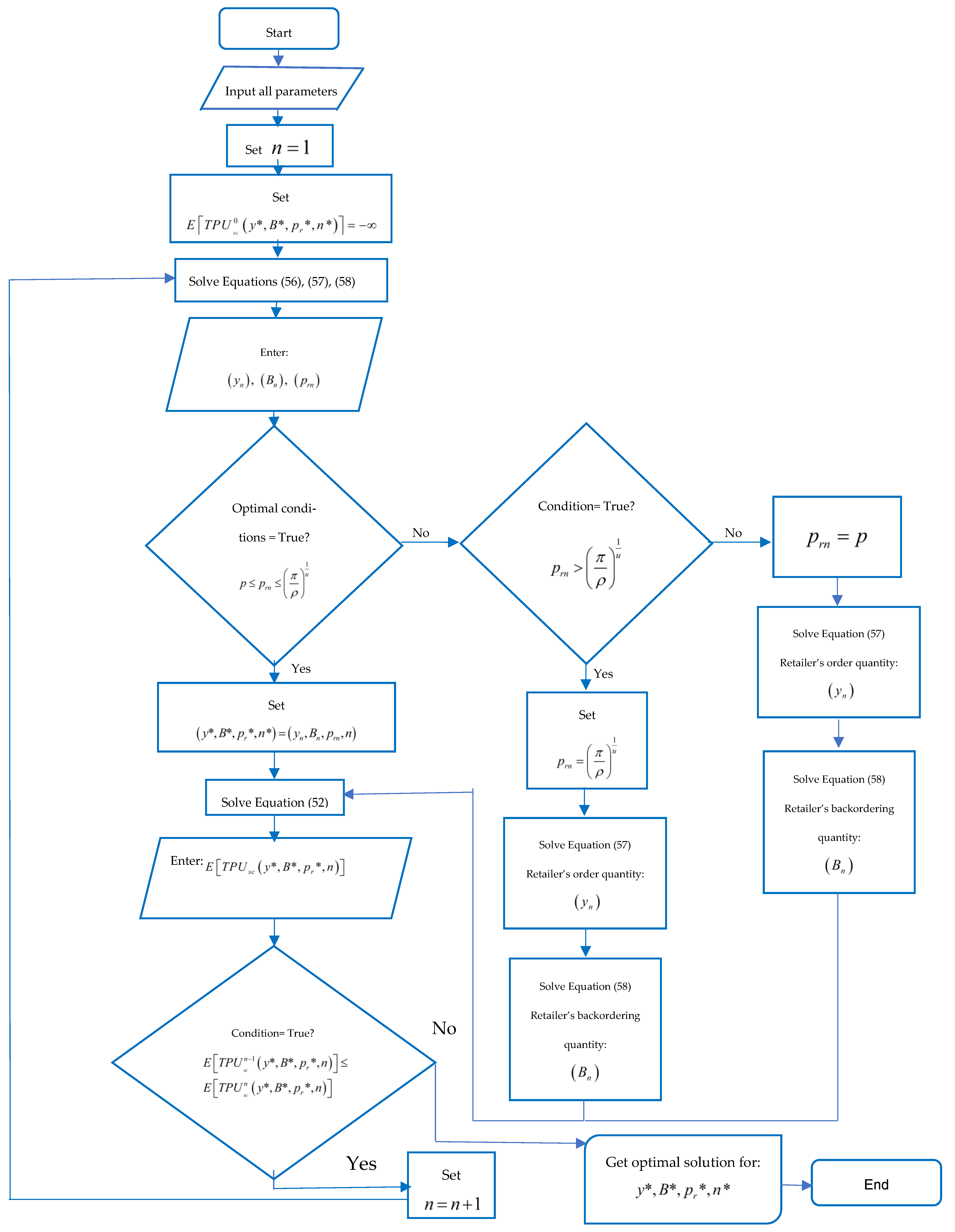
5.2. Algorithm for Finding the Optimal Solution

The values of y , B and p r which maximize the objective function E [ T P U s c ( y , B , p r ) ] are determined through the following Algorithm 1:
Algorithm 1 Algorithm for Finding the Optimal Solution
Step 1. Provide all input parameters of the inventory system, set n = 1 and E [ T P U s c 0 ( y * , B * , p r * , n * ) ] = .
Step 2. Compute the retailer’s order quantity ( y n ) , the retailer’s backordering quantity ( B n ) and the selling price ( p r n ) by solving simultaneously Equations (56)–(58).
Step 3. If the optimality conditions are satisfied then go to Step 4. If not go to Step 10.
Step 4. If p p r n ( π ρ ) 1 u then go to Step 6. If not go to Step 5.
Step 5. If p r n > ( π ρ ) 1 u then set p r n = ( π ρ ) 1 u , calculate the retailer’s order quantity ( y n ) with Equation (57) and the retailer’s backordering quantity ( B n ) with Equation (58) and go to Step 6. Otherwise, set p r n = p and determine the retailer’s order quantity ( y n ) with Equation (57) and the retailer’s backordering quantity ( B n ) with Equation (58) and go to Step 6.
Step 6. Set the solution as ( y * , B * , p r * , n * ) = ( y n , B n , p r n , n ) .
Step 7. Compute the expected total profit per unit of time E [ T P U s c ( y * , B * , p r * , n ) ] with Equation (52).
Step 8. If E [ T P U s c n 1 ( y * , B * , p r * , n ) ] E [ T P U s c n ( y * , B * , p r * , n ) ] then set n = n + 1 and go to Step 2. Otherwise, go to Step 9.
Step 9. Report the optimal solution as y * , B * , p r * , n * and E [ T P U s c n ( y * , B * , p r * , n ) ] .
Step 10. Stop.
A flow diagram of the algorithm is represented in Figure 7.

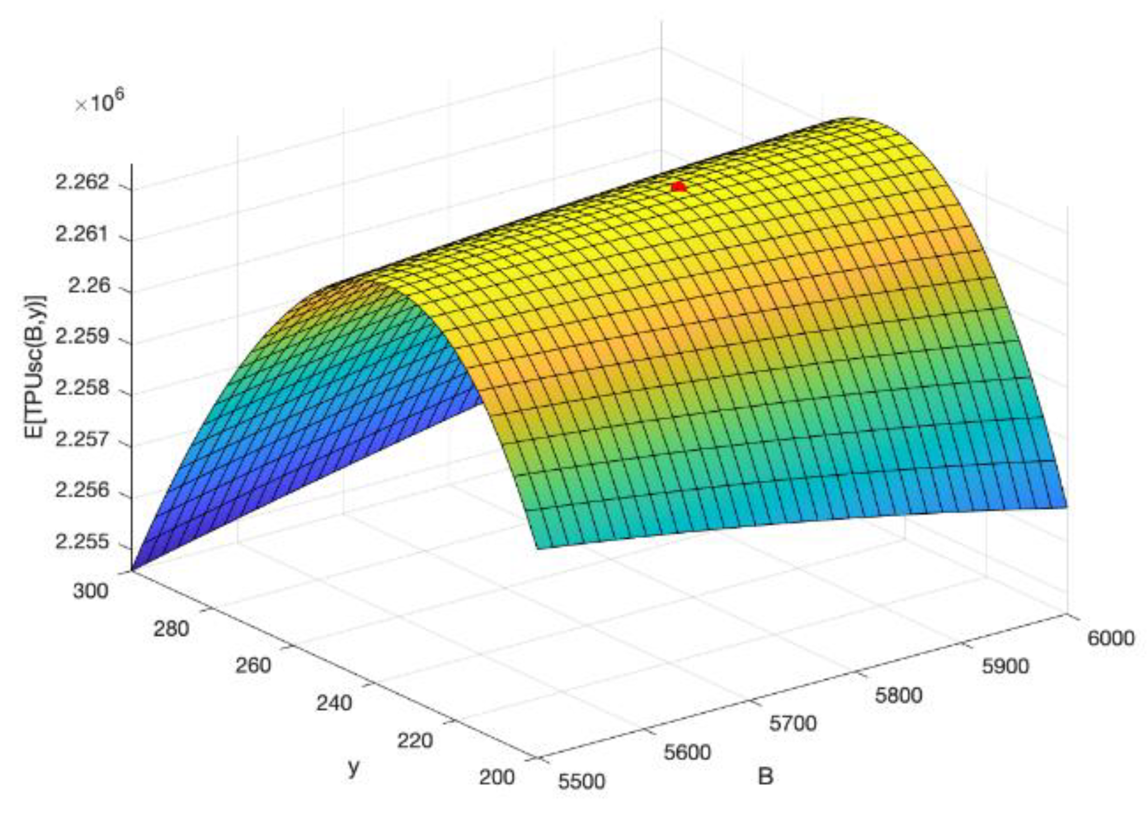
6. Numerical Example

The proposed inventory model for growing items is illustrated through a numerical example for a supply chain which considers a farmer, a processor, and a retailer. It is for a specific type of newborn animal: chicks. The farmer buys and grows newborn items, and then ships them to a processor for slaughtering, cutting, and packaging. The processor then ships an integer number of batches of the processed items to the retailer.
The algorithm was coded in Lingo/Win64 15.0.63, LINDO Systems Inc., Chicago, USA. API Version 9.0.21.20.240. The numerical example and sensitivity analysis were carried out on a computer with a macOS Monterey version 12.5.1. MacBook Pro (2016). 2.9 GHz Intel Core i5 dual-core processor, 8 GB 2133 MHz LPDDR3 memory, Macintosh HD boot disk-data, Apple Inc., California, USA.
Example 1.
This example considers some data of Sebatjane and Adetunji [7] which are:
p v = 20 USD/g, p p = 30 USD/g, p = 10 USD/g, K f = 40 , 000 USD/cycle, K p = 60 , 000 USD/cycle, K r = 80 , 000 USD/cycle, c f = 10 USD/g, m f = 2 USD/g, h s = 15 USD/g/year, h r = 20 USD/g/year, z = 0.5 USD/g, P = 12500 , 500 g/year, α = 51 g, β = 5 , λ = 6.2 /year, a = 0.9 , w 0 = 8.5 g, w 1 = 45 g, and x ~ U [ 0 , 0.05 ] .
Here, the inspection rate is r = 20 , 000 g/year. Additionally, new parameters are given as follows: the processor’s purchasing cost is p f = 25 USD/g, the farmer’s holding cost of the growing live items is h l = 12 USD/g/year, the processor´s processing cost is p c = 5 USD/g/year, the retailer’s shortage cost is b = 4 USD/g/year. Assume that the demand rate of the growing items follows a polynomial function given by D ( p r ) = π ρ p r u with values of π = 10 , 000 , and ρ = 10 .
The input parameters related to carbon emissions are: θ = 0.0045 /tons, p p = 25 tons/year, p = 5 tons/year, K f = 20 , 000 tons/year, K p = 30 , 000 tons/year, K r = 40 , 000 tons/year, c f = 6 tons/year, m f = 1 tons/year, h l = 10 tons/year, h s = 13 tons/year, h r = 18 tons/year, p c = 2 tons/year, and z = 0.25 . The percentage of imperfect growing items follows a uniform distribution ( x ~ U [ γ , δ ] ) with the following probability density function g ( x ) = { 1 δ γ   γ x δ 0   otherwise . Considering x ~ U [ 0 , 0.05 ] then x ~ g ( x ) = { 20   0 x 0.05 0   otherwise . The expected values of E [ x ] and E [ ( 1 x ) 2 ] are computed as follows:
E [ x ] = γ δ x f ( x ) d x = γ + δ 2 = 0 + 0.05 2 = 0.025
E [ ( 1 x ) 2 ] = γ δ ( 1 x ) 2 f ( x ) d x = γ 2 + γ δ + δ 2 3 + 1 γ δ
E [ ( 1 x ) 2 ] = 0 2 + 0 ( 0.05 ) + ( 0.05 ) 2 3 + 1 0 0.05 = 0.95083333
The fraction of the live items which survive throughout the growth period ( a ) is assumed to be random and variable uniformly distributed over [ 0.8 , 1 ] . Its probability density function is given by the following probability density function g ( a ) = { 5   0.8 a 1 1   otherwise . This implies that: E [ a ] = 0.8 1 5 a   d a = 5 [ ( 1 2 + 0.8 2 ) 2 ] = 0.9 .
With the proposed algorithm, it is obtained the optimal solution: E [ T P U s c * ( y * , B * , p r * , n * ) ] = 2 , 262 , 526 USD/YEAR, order quantity y * = 241.1837 , backordering quantity B * = 5791.250 , selling price   p r * = 522.0497 and the number of shipments n * = 1 . The Figure 8, Figure 9 and Figure 10 show graphically the concavity property of the expected total profit with respect to pairs of decision variables B and p r ; p r and y ; and B and y , respectively. It is important to remark that the units of y * are different from the units of B * . The lot size y * is the number of newborns of growing items, while B * is an amount of weight in grams. For example, Q 1 = ( y ) ( w 1 ) = 10 , 853.26 gr. Therefore, the constraint is satisfied: B Q 1 = 5791.25 gr. < 10,853.26 gr.

7. Sensitivity Analysis

This section provides a sensitivity analysis on the supply chain system in order to investigate the effects of changing the input parameters on the expected total profit per unit of time ( E [ T P U s c * ] ) , order quantity ( y * ) , backordering quantity ( B * ) , selling price ( p r * ) , and the number of shipments ( n * ) of the growing items. The sensitivity analysis takes into consideration the numerical example data when one parameter is changed while the others are kept the same value. The sensitivity analysis results are given in Table 2, Table 3, Table 4, Table 5, Table 6 and Table 7.

8. Managerial Insights

The following managerial insights through the sensitivity analysis are provided. Based on the behavioral changes, as reflected in Table 2, Table 3, Table 4, Table 5, Table 6 and Table 7:
(1)
Changes in feeding cost c f have a significant effect on the total profit per unit of time ( E [ T P U s c ] ) : the company needs to pay attention to this cost.
(2)
Variations in holding costs in the three stages of the supply chain h l , h s , h r have a substantial impact on the total profit per unit of time ( E [ T P U s c ] ) : the company needs to pay attention to these costs.
(3)
Processor’s purchasing cost p f retailer’s purchasing cost p p , and amount of carbon emissions produced during farmer’s mortality process m f have not influence on the total profit per unit of time ( E [ T P U s c ] ) .
(4)
Changes to all input parameters do not affect the number of shipments made by the processor ( n ) to the retailer during a single processing run.
(5)
The total profit value per unit of time ( E [ T P U s c ] ) is susceptible to the demand parameters π , ρ , u and less sensitive to other parameters. On the one hand, the higher value of the scale parameter of demand π , the higher value of ( E [ T P U s c ] ) due to the fact that demand increases, therefore, the sales increment and this leads to high profits, which is suitable for the company.
(6)
The value of the order quantity ( y ) is more sensitive to the parameters π , ρ , K f , K p , K r , h l , h s , h r and less sensitive to other parameters. The higher value of the parameter of h r , the smaller value of the order quantity y .
(7)
The value of backordering quantity ( B ) is more sensitive to the parameters π , K p , K r , h s , h r , b , p and less sensitive to other parameters. The higher value of π , the smaller value of backordering quantity ( B ).
(8)
The value of selling price ( p r ) is more sensitive to the parameters π , ρ , u and less sensitive to other parameters. The higher value of the parameter of π , the higher value of selling price ( p r ). This means that as demand scale parameter π increases, the company must raise selling price, which also directly impacts positively in the expected total profit per unit of time ( E [ T P U s c ] ) .
(9)
Variations in carbon emissions parameters regularly influence the expected total profit per unit of time ( E [ T P U s c ] ) , except for the amount of carbon emissions produced during the farmer’s mortality process m f . It is essential to pay attention to this point so that the company does not generate so many emissions and it does not pay too much carbon tax.

9. Conclusions and Future Research

The significant contribution made by the research presented in this paper is the incorporation of mortality, imperfect quality, shortages, and the optimization of selling price into a three-echelon supply chain for growing items. The mortality as the same as the imperfect quality follows a uniform distribution with a probability density function. The three-echelon supply chain includes agricultural, processing, and retail operations to represent a food production supply chain. Another significant aspect of the research work is the consideration of carbon emissions since it is currently of great importance to consider developing inventory models concerned about the environment. An algorithm is developed to solve the inventory model to generate the optimal solution for order quantity, backordering quantity, selling price, and the number of shipments that maximizes the expected total profit per unit of time. A numerical example is solved to test the applicability of the proposed inventory model. Other popular EOQ extensions can be incorporated, such as maintenance issues, permissible delays in payments, and the inclusion of more echelons in the supply chain. The methane and nitrous oxide, besides the carbon emission scenario, can be an extension of the proposed inventory model in the virtue of the environmental perspective to save nature along with the sustainable movement of the inventory in different places. This study considered only a supply chain with three stages and one member for each. If more stages and network members are required, then it will be a significant research area to explore. Additionally, the deterioration plays an essential role in growing items. An interesting investigation on a replenishment policy for deteriorating products that determines sale price, investment in preservation technology, and replenishment cycle time by maximizing the total profit as it was achieved by Dey et al. [79]. For further development, researchers can consider an optimum investment to reduce the rate of deterioration by preservation technology considering their lifespan as it was achieved in Saha et al. [80].

Author Contributions

Conceptualization, C.G.D.-l.-C.-M. and L.E.C.-B.; Methodology, C.G.D.-l.-C.-M., L.E.C.-B., B.M., N.R.S., R.E.B.-D., I.d.J.L.-H., A.C.-M. and G.T.-G.; Software, C.G.D.-l.-C.-M. and L.E.C.-B.; Validation, L.E.C.-B., B.M., N.R.S., R.E.B.-D., I.d.J.L.-H., A.C.-M. and G.T.-G.; Formal analysis, C.G.D.-l.-C.-M., L.E.C.-B., B.M., N.R.S., R.E.B.-D., I.d.J.L.-H., A.C.-M. and G.T.-G.; Investigation, C.G.D.-l.-C.-M., L.E.C.-B., B.M., N.R.S., R.E.B.-D., I.d.J.L.-H., A.C.-M. and G.T.-G.; Data curation, C.G.D.-l.-C.-M., L.E.C.-B., B.M., N.R.S., R.E.B.-D., I.d.J.L.-H., A.C.-M. and G.T.-G.; Writing—original draft, C.G.D.-l.-C.-M.; Writing—review and editing, L.E.C.-B.; Visualization, C.G.D.-l.-C.-M.; Supervision, L.E.C.-B. All authors have read and agreed to the published version of the manuscript.

Funding

The APC was funded by Tecnológico de Monterrey.

Institutional Review Board Statement

Not applicable.

Informed Consent Statement

Not applicable.

Data Availability Statement

Not applicable.

Conflicts of Interest

The authors declare no conflict of interest.

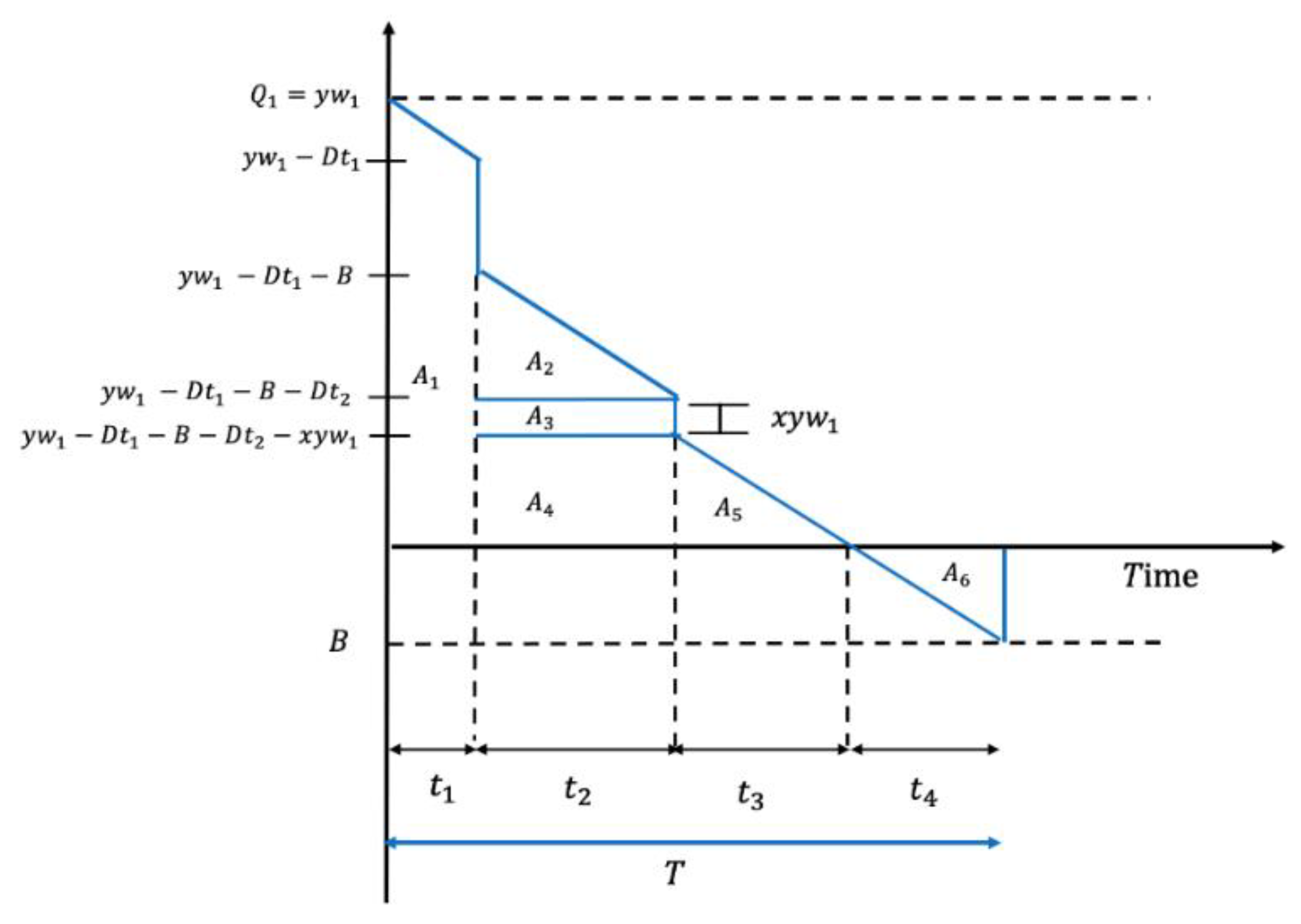
Appendix A. Determination of the Retailer’s Expected Holding Cost E [ H C h r ]

The retailer’s expected holding cost is computed by the multiplication of the unit holding cost ( h r ) and the total inventory accumulated during periods t 1 + t 2 + t 3 . The area is calculated by the sum of the areas A 1 + A 2 + A 3 + A 4 + A 5 , which are the positive inventory units. Based on the Figure A1 the five areas ( A 1 , A 2 , A 3 , A 4 , A 5 ) are defined as follows:
The area A 1 is found as follows:
A 1 = ( B + b ) h 2 = ( y w 1 + y w 1 D ( p r ) t 1 ) t 1 2 = ( 2 y w 1 D ( p r ) t 1 ) t 1 2 = [ 2 y w 1 D ( p r ) ( B r D ( p r ) ) ] B r D ( p r ) 2
A 1 = [ 2 y w 1 ( D ( p r ) B r D ( p r ) ) ] B r D ( p r ) 2 = y w 1 ( B r D ( p r ) ) D ( p r ) 2 ( B r D ( p r ) ) 2
The area A 2 is defined in this way:
A 2 = t 2 D ( p r ) t 2 2 = D ( p r ) t 2 2 2 = D ( p r ) ( y w 1 D ( p r ) t 1 B r ) 2 2 = D ( p r ) ( y w 1 D ( p r ) B r D ( p r ) B r ) 2 2 = D ( p r ) [ y w 1 ( 1 + D ( p r ) r D ( p r ) ) B r ] 2 2
A 2 = D ( p r ) 2 r 2 [ y w 1 ( 1 1 D ( p r ) r ) B ] 2 = D ( p r ) 2 [ y w 1 r B r D ( p r ) ] 2
A 2 = D ( p r ) 2 r 2 [ y w 1 ( 1 + D ( p r ) r D ( p r ) ) B ] 2 = D ( p r ) 2 r 2 [ y w 1 ( D ( p r ) + r D ( p r ) r D ( p r ) ) B ] 2 = D ( p r ) 2 r 2 [ y w 1 ( r r D ( p r ) ) B ] 2
Figure A1. Inventory behavior through time.
Mathematics 10 04684 g0a1
The area A 3 is obtained as follows:
A 3 = t 2 x y w 1 = ( y w 1 D ( p r ) t 1 B r ) x y w 1 = ( y w 1 D ( p r ) t 1 B r ) x y w 1 = [ y w 1 r D ( p r ) r ( B r D ( p r ) ) B r ] x y w 1
A 3 = [ y w 1 r B D + B ( r D ( p r ) ) r ( r D ( p r ) ) ] x y w 1 = [ y w 1 r B D ( p r ) + B r B D ( p r ) r ( r D ( p r ) ) ] x y w 1 = [ y w 1 r B ( r D ( p r ) ) ] x y w 1
The area A 4 is given by:
A 4 = t 2 [ y w 1 D ( p r ) t 1 B D ( p r ) t 2 x y w 1 ] = ( y w 1 r B r D ( p r ) ) [ y w 1 D ( p r ) ( B r D ( p r ) ) B D ( p r ) ( y w 1 r B r D ( p r ) ) x y w 1 ]
A 4 = ( y w 1 r B r D ( p r ) ) [ y w 1 D ( p r ) ( y w 1 r ) B x y w 1 ] = ( y w 1 r B r D ( p r ) ) [ y w 1 ( 1 D ( p r ) r x ) B ]
The area A 5 is determined in this manner:
A 5 = t 3 [ y w 1 D t 1 B D ( p r ) t 2 x y w 1 ] 2 = t 3 [ y w 1 D ( p r ) ( t 1 + t 2 ) B x y w 1 ] 2 = [ y w 1 D ( p r ) ( t 1 + t 2 ) B x y w 1 ] 2 2 D ( p r )
A 5 = [ y w 1 D ( p r ) ( y w 1 r ) B x y w 1 ] 2 2 D ( p r ) = [ y w 1 ( 1 D ( p r ) r x ) B ] 2 2 D ( p r )
The total inventory accumulated ( T I A ) during t 1 + t 2 + t 3 is computed in this way: ( T I A ) = A 1 + A 2 + A 3 + A 4 + A 5 . Substituting the corresponding areas,
T I A = y w 1 ( B r D ( p r ) ) D ( p r ) 2 ( B r D ( p r ) ) 2 + D ( p r ) 2 [ y w 1 r B r D ( p r ) ] 2 + ( y w 1 r B r D ( p r ) ) x y w 1 + ( y w 1 r B r D ( p r ) ) [ y w 1 ( 1 D ( p r ) r x ) B ] + [ y w 1 ( 1 D ( p r ) r x ) B ] 2 2 D ( p r )
Simplifying,
T I A = y w 1 B r + y 2 w 1 2 D ( p r ) 2 r 2 + y 2 w 1 2 r y 2 w 1 2 D ( p r ) r 2 2 y w 1 B r + B 2 r D ( p r )
T I A = y 2 w 1 2 r y 2 w 1 2 D ( p r ) 2 r 2 y w 1 B r + B 2 r D ( p r )
T I A = y w 1 r [ y w 1 ( 1 D ( p r ) 2 r ) B ] + B 2 r D ( p r )
T I A = y w 1 r [ y w 1 ( 1 D ( p r ) 2 r ) B ] + B 2 r D ( p r ) + [ y w 1 ( 1 D ( p r ) r x ) B ] 2 2 D ( p r )
Taking the expected value of the total inventory accumulated ( T I A ), the following expression is obtained:
E [ T I A ] = y w 1 r [ y w 1 ( 1 D ( p r ) 2 r ) B ] + B 2 r D ( p r ) + [ y w 1 ( 1 D ( p r ) r E [ x ] ) B ] 2 2 D ( p r )
Finally, the expected holding cost E [ H C h r ] is given by:
E [ H C h r ] = h r { y w 1 r [ y w 1 ( 1 D ( p r ) 2 r ) B ] + B 2 r D ( p r ) + [ y w 1 ( 1 D ( p r ) r E [ x ] ) B ] 2 2 D ( p r ) }

Appendix B. Determination of the Retailer’s Backordering Cost B C r

The backordering cost is computed by the multiplication of the unit backordering cost b and the total shortages accumulated during t 4 , and this is the area A 6 shown below level zero in Figure 10. This area A 6 is found as follows:
A 6 = ( t 4 ) B 2 = ( B D ( p r ) ) B 2 = B 2 2 D ( p r )
Then, the backordering cost B C r is given by:
B C r = b ( B 2 2 D ( p r ) )

Appendix C. Sufficient Conditions for the Optimality
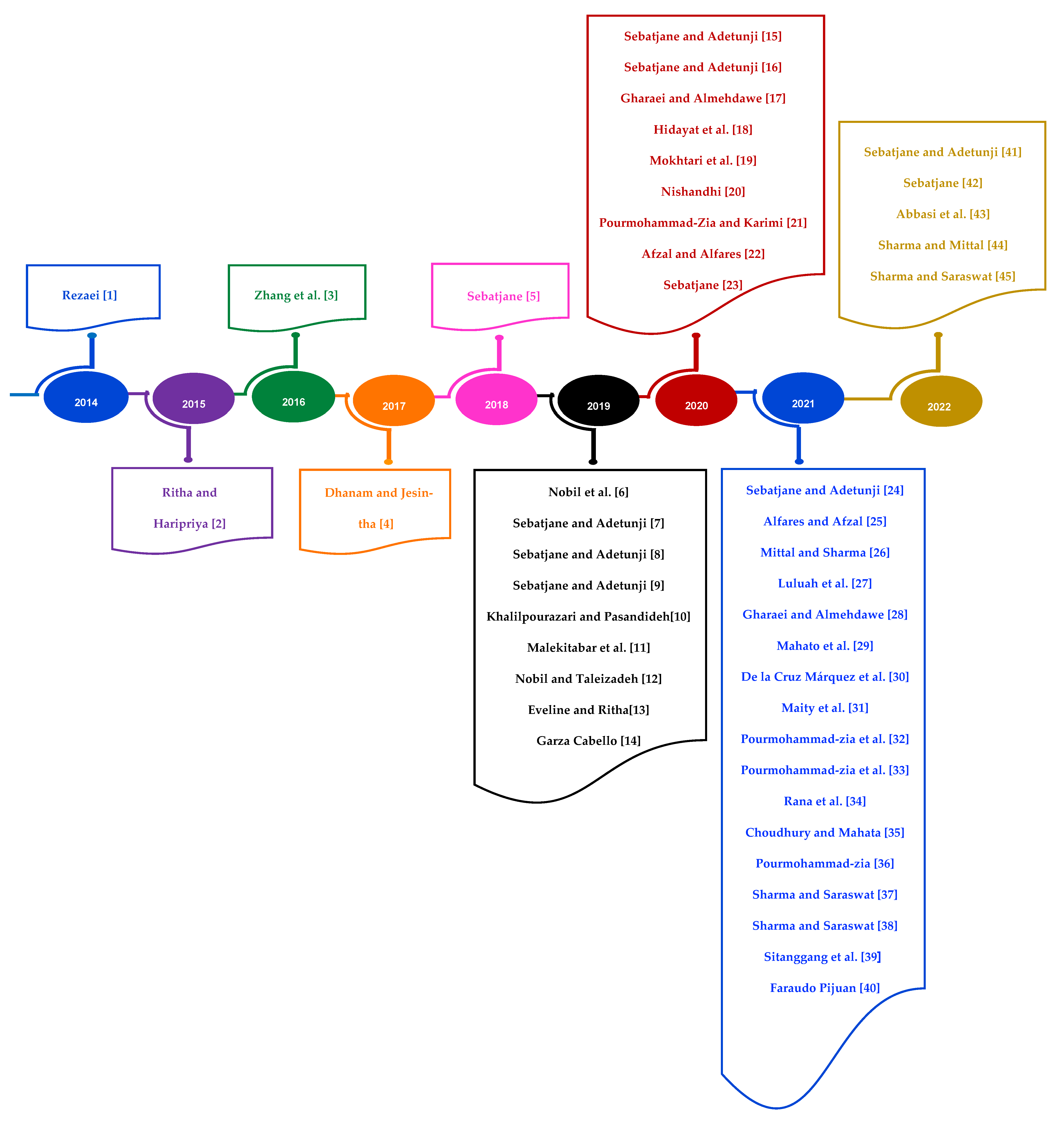
The final equations for the direct and cross second-order partial derivatives are provided below.
The direct second order partial derivatives:
The second order partial derivative of Equation (52) with respect to y is expressed as:
2 E [ T P U s c ( y , B , p r ) ] y 2 = 1 ( 1 E [ x ] ) { 2 ( π ρ p r u ) y 3 w 1 [ ( K f n + K p n + K r ) + θ ( K f n + K p n + K r ) ] b B 2 y 3 w 1 ( h r + θ h r ) [ 2 B 2 ( π ρ p r u ) y 3 w 1 ( r ( π ρ p r u ) ) + B 2 y 3 w 1 ] } < 0
The second order partial derivative of Equation (52) with respect to B is found as follows:
2 E [ T P U s c ( y , B , p r ) ] B 2 = 1 y w 1 ( 1 E [ x ] ) { ( h r + θ h r ) [ 3 ( π ρ p r u ) r ] ( r ( π ρ p r u ) ) + b } < 0
The second order partial derivative of Equation (52) with respect to p r is presented below:
2 E [ T P U s c ( y , B , p r ) ] p r 2 = ρ u p r u 1 ( u + 1 ) ( ρ u p r u 1 ) w 1 ( 1 E [ x ] ) { ( h r + θ h r ) [ 2 B 2 r ( ρ u p r u 1 ) y ( ρ p r u + r π ) 3 ] }      + { ( p + θ p ) w 0 ( K f + θ K f ) n y + p p w 1 n ( θ p f E [ a ] ) w 1 ( K p + θ K p ) n y      ( p c E [ a ] + θ p c E [ a ] ) w 1 + p v E [ x ] w 1 ( p p + θ p p ) w 1 ( K r + θ K r ) y ( z + θ z ) w 1      [ ( c f E [ a ] + θ c f E [ a ] ) + [ ( m f + θ m f ) ( 1 E [ a ] ) ] + ( h l + θ h l ) ] { α T f + α λ [ ln ( 1 + β e λ T f ) ln ( 1 + β ) ] }      ( h s + θ h s ) [ y w 1 2 ( 2 n ) ] 2 P ( h r + θ h r ) [ y w 1 2 E [ x ] r + B 2 y ( ρ p r u + r π ) [ 1 + ( π ρ p r u ) ( ρ p r u + r π ) ] ] } [ ρ u p r u 2 ( 1 u ) w 1 ( 1 E [ x ] ) ]
The second order cross partial derivatives:
The second order cross partial derivative ( 2 y B ) of Equation (52) is given by:
2 E [ T P U s c ( y , B , p r ) ] y B = 1 ( 1 E [ x ] ) { b B y 2 w 1 + ( h r + θ h r ) [ 2 ( π ρ p r u ) B y 2 w 1 ( r ( π ρ p r u ) ) + B y 2 w 1 ] }
The second order cross partial derivative ( 2 y p r ) of Equation (52) is as below:
2 E [ T P U s c ( y , B , p r ) ] y p r = ( ρ u p r u 1 ) w 1 ( 1 E [ x ] ) { ( K f + θ K f ) n y 2 + ( K p + θ K p ) n y 2 + ( K r + θ K r ) y 2 ( h s + θ h s ) [ w 1 2 ( 2 n ) ] 2 P ( h r + θ h r ) { B 2 y 2 ( ρ p r u + r π ) [ 1 + ( π ρ p r u ) ( ρ p r u + r π ) ] + w 1 2 ( E [ x ] ) r } }
The second order cross partial derivative ( 2 B y ) of Equation (52) is written in this manner:
2 E [ T P U s c ( y , B , p r ) ] B y = 1 ( 1 E [ x ] ) { b B y 2 w 1 + ( h r + θ h r ) [ 2 ( π ρ p r u ) B y 2 w 1 ( r ( π ρ p r u ) ) + B y 2 w 1 ] }
The second order cross partial derivative ( 2 B p r ) of Equation (52) is shown in this way:
2 E [ T P U s c ( y , B , p r ) ] B p r = ( h r + θ h r ) ( ( ρ u p r u 1 ) ( 1 E [ x ] ) ) 2 B y w 1 ( ρ p r u + r π ) [ 1 + ( π ρ p r u ) ( ρ p r u + r π ) ]
The second order cross partial derivative ( 2 p r y ) of Equation (52) is given by:
2 E [ T P U s c ( y , B , p r ) ] p r y = ( ρ u p r u 1 ) w 1 ( 1 E [ x ] ) { ( K f + θ K f ) n y 2 + ( K p + θ K p ) n y 2 + ( K r + θ K r ) y 2 ( h s + θ h s ) [ w 1 2 ( 2 n ) ] 2 P ( h r + θ h r ) { B 2 y 2 ( ρ p r u + r π ) [ 1 + ( π ρ p r u ) ( ρ p r u + r π ) ] + w 1 2 ( E [ x ] ) r } }
The second order cross partial derivative ( 2 p r B ) of Equation (52) is obtained by:
2 E [ T P U s c ( y , B , p r ) ] p r B = ( h r + θ h r ) ( ( ρ u p r u 1 ) ( 1 E [ x ] ) ) 2 B y w 1 ( ρ p r u + r π ) [ 1 + ( π ρ p r u ) ( ρ p r u + r π ) ]
Optimality:
The Hessian matrix of the objective function, given by
H = [ 2 E [ T P U s c ( y , B , p r ) ] y 2 2 E [ T P U s c ( y , B , p r ) ] y B 2 E [ T P U s c ( y , B , p r ) ] y p r 2 E [ T P U s c ( y , B , p r ) ] B y 2 E [ T P U s c ( y , B , p r ) ] B 2 2 E [ T P U s c ( y , B , p r ) ] B p r 2 E [ T P U s c ( y , B , p r ) ] s y 2 E [ T P U s c ( y , B , p r ) ] s B 2 E [ T P U s c ( y , B , p r ) ] p r 2 ]
The necessary conditions for optimality through the Hessian matrix H are as follows: D e t ( H 1 ) < 0 , D e t ( H 2 ) > 0 and D e t ( H 3 ) < 0 , where H 1 , H 2 , and H 3 are the following matrixes:
H 1 = [ 2 E [ T P U s c ( y , B , p r ) ] y 2 ]  
H 2 = [ 2 E [ T P U s c ( y , B , p r ) ] y 2 2 E [ T P U s c ( y , B , p r ) ] y B 2 E [ T P U s c ( y , B , p r ) ] B y 2 E [ T P U s c ( y , B , p r ) ] B 2 ]
H 3 = [ 2 E [ T P U s c ( y , B , p r ) ] y 2 2 E [ T P U s c ( y , B , p r ) ] y B 2 E [ T P U s c ( y , B , p r ) ] y p r 2 E [ T P U s c ( y , B , p r ) ] B y 2 E [ T P U s c ( y , B , p r ) ] B 2 2 E [ T P U s c ( y , B , p r ) ] B p r 2 E [ T P U s c ( y , B , p r ) ] s y 2 E [ T P U s c ( y , B , p r ) ] s B 2 E [ T P U s c ( y , B , p r ) ] p r 2 ]
Accordingly,
D e t ( H 1 ) = 2 E [ T P U s c ( y , B , p r ) ] y 2 = 1 ( 1 E [ x ] ) { 2 ( π ρ p r u ) y 3 w 1 [ ( K f n + K p n + K r ) + θ ( K f n + K p n + K r ) ] b B 2 y 3 w 1 ( h r + θ h r ) [ 2 B 2 ( π ρ p r u ) y 3 w 1 ( r ( π ρ p r u ) )         + B ( r ( π ρ p r u ) r E [ x ] ) y 2 + [ y w 1 ( r ( π ρ p r u ) r E [ x ] ) B ] 2 y 3 w 1 [ y w 1 ( r ( π ρ p r u ) r E [ x ] ) B ] ( r ( π ρ p r u ) r E [ x ] ) y 2 ] } < 0
D e t ( H 2 ) = ( 2 E [ T P U s c ( y , B , p r ) ] y 2 ) ( 2 E [ T P U s c ( y , B , p r ) ] B 2 ) ( 2 E [ T P U s c ( y , B , p r ) ] y B ) 2 > 0
D e t ( H 2 ) = ( 1 ( 1 E [ x ] ) { 2 ( π ρ p r u ) y 3 w 1 [ ( K f n + K p n + K r ) + θ ( K f n + K p n + K r ) ] b B 2 y 3 w 1 ( h r + θ h r ) [ 2 B 2 ( π ρ p r u ) y 3 w 1 ( r ( π ρ p r u ) ) + B 2 y 3 w 1 ] } ) ( 1 y w 1 ( 1 E [ x ] ) { ( h r + θ h r ) [ 3 ( π ρ p r u ) r ] ( r ( π ρ p r u ) ) + b } ) ( 1 ( 1 E [ x ] ) { b B y 2 w 1 + ( h r + θ h r ) [ 2 ( π ρ p r u ) B y 2 w 1 ( r ( π ρ p r u ) ) + B y 2 w 1 ] } ) 2 > 0
D e t ( H 3 ) = ( 2 E [ T P U s c ( y , B , p r ) ] y 2 ) ( 2 E [ T P U s c ( y , B , p r ) ] B 2 ) ( 2 E [ T P U s c ( y , B , p r ) ] p r 2 ) + ( 2 E [ T P U s c ( y , B , p r ) ] B y ) ( 2 E [ T P U s c ( y , B , p r ) ] s B ) ( 2 E [ T P U s c ( y , B , p r ) ] y p r )   + ( 2 E [ T P U s c ( y , B , p r ) ] s y ) ( 2 E [ T P U s c ( y , B , p r ) ] y B ) ( 2 E [ T P U s c ( y , B , p r ) ] B p r ) ( 2 E [ T P U s c ( y , B , p r ) ] y p r ) ( 2 E [ T P U s c ( y , B , p r ) ] B 2 ) ( 2 E [ T P U s c ( y , B , p r ) ] p r y ) ( 2 E [ T P U s c ( y , B , p r ) ] B p r ) ( 2 E [ T P U s c ( y , B , p r ) ] s B ) ( 2 E [ T P U s c ( y , B , p r ) ] y 2 ) ( 2 E [ T P U s c ( y , B , p r ) ] p r 2 ) ( 2 E [ T P U s c ( y , B , p r ) ] y B ) ( 2 E [ T P U s c ( y , B , p r ) ] B y )   <   0
The analysis proves that the objective function 2 E [ T P U s c ( y , B , p r ) ] is concave. It shows that the Hessian is negative-definite. Therefore, the optimal solution for the decision variables ( y * , B * , p r * ) exists and maximizes the expected total profit per unit of time.

References

  1. Rezaei, J. Economic order quantity for growing items. Int. J. Prod. Econ. 2014, 155, 109–113. [Google Scholar] [CrossRef]
  2. Ritha, W.; Haripriya, S. Inventory model on organic poultry farming. Int. J. Res. Eng. Appl. Sci. 2015, 5, 30–38. [Google Scholar]
  3. Zhang, Y.; Li, L.Y.; Tian, X.Q.; Feng, C. Inventory management research for growing items with carbon-constrained. In Proceedings of the 2016 35th Chinese Control Conference (CCC), Chengdu, China, 27–29 July 2016; pp. 9588–9593. [Google Scholar]
  4. Dhanam, K.; Jesintha, W. Fuzzy inventory model for slow and fast growing items with deterioration constraints in a single period. Int. J. Manag. Soc. Sci. 2017, 5, 308–317. [Google Scholar]
  5. Sebatjane, M. Selected Deterministic Models for Lot Sizing of Growing Items Inventory. Master’s Thesis, University of Pretoria, Pretoria, South Africa, 2018. [Google Scholar]
  6. Nobil, A.H.; Sedigh, A.H.A.; Cárdenas-Barrón, L.E. A generalized economic order quantity inventory model with shortage: Case study of a poultry farmer. Arab. J. Sci. Eng. 2019, 44, 2653–2663. [Google Scholar] [CrossRef]
  7. Sebatjane, M.; Adetunji, O. Economic order quantity model for growing items with imperfect quality. Oper. Res. Perspect. 2019, 6, 100088. [Google Scholar] [CrossRef]
  8. Sebatjane, M.; Adetunji, O. Economic order quantity model for growing items with incremental quantity discounts. J. Ind. Eng. Int. 2019, 15, 545–556. [Google Scholar] [CrossRef] [Green Version]
  9. Sebatjane, M.; Adetunji, O. Three-echelon supply chain inventory model for growing items. J. Model. Manag. 2019, 15, 567–587. [Google Scholar] [CrossRef]
  10. Khalilpourazari, S.; Pasandideh, S.H.R. Modeling and optimization of multi-item multi-constrained EOQ model for growing items. Knowl.-Based Syst. 2019, 164, 150–162. [Google Scholar] [CrossRef]
  11. Malekitabar, M.; Yaghoubi, S.; Gholamian, M.R. A novel mathematical inventory model for growing-mortal items (case study: Rainbow trout). Appl. Math. Model. 2019, 71, 96–117. [Google Scholar] [CrossRef]
  12. Nobil, A.H.; Taleizadeh, A.A. Economic order quantity model for growing items with correct order size. Modeling Eng. 2019, 17, 123–129. [Google Scholar]
  13. Eveline, J.C.; Ritha, W. Economic order quantity inventory model for poultry farming with shortages, screening, and affiliated costs considerations. Impact J. 2019, 7, 141–148. [Google Scholar]
  14. Garza-Cabello, E. Modelo de Inventarios para Ítems Con Crecimiento, Calidad Imperfecta y Faltantes Planeados. Master’s Thesis, Tecnológico de Monterrey, Monterrey, México, 2019. [Google Scholar]
  15. Sebatjane, M.; Adetunji, O. A three-echelon supply chain for economic growing quantity model with price-and freshness-dependent demand: Pricing, ordering and shipment decisions. Oper. Res. Perspect. 2020, 7, 100153. [Google Scholar] [CrossRef]
  16. Sebatjane, M.; Adetunji, O. Optimal inventory replenishment and shipment policies in a four-echelon supply chain for growing items with imperfect quality. Prod. Manuf. Res. 2020, 8, 130–157. [Google Scholar] [CrossRef]
  17. Gharaei, A.; Almehdawe, E. Economic growing quantity. Int. J. Prod. Econ. 2020, 223, 107517. [Google Scholar] [CrossRef]
  18. Hidayat, Y.A.; Riaventin, V.N.; Jayadi, O. Economic order quantity model for growing items with incremental quantity discounts, capacitated storage facility, and limited budget. J. Tek. Ind. 2020, 22, 1–10. [Google Scholar] [CrossRef]
  19. Mokhtari, H.; Salmasnia, A.; Asadkhani, J. A new production-inventory planning model for joint growing and deteriorating items. Int. J. Supply Oper. Manag. 2020, 7, 1–16. [Google Scholar]
  20. Nishandhi, F. An economic order quantity model for growing items with imperfect quality and budget capacity constraint to limit the purchase. Solid State Technol. 2020, 63, 7852–7858. [Google Scholar]
  21. Pourmohammad-Zia, N.; Karimi, B. Optimal replenishment and breeding policies for growing items. Arab. J. Sci. Eng. 2020, 45, 7005–7015. [Google Scholar] [CrossRef]
  22. Afzal, A.R.; Alfares, H.K. An inventory model for growing items with quality inspections and permissible shortages. In Proceedings of the 5th NA International Conference on Industrial Engineering and Operations Management, Detroit, MI, USA, 10–14 August 2020; pp. 1153–1160. [Google Scholar]
  23. Sebatjane, M. Inventory Management for Growing Items in Multi-Echelon Supply Chains. Ph.D. Thesis, University of Pretoria, Pretoria, South Africa, 2020. [Google Scholar]
  24. Sebatjane, M.; Adetunji, O. Optimal lot-sizing and shipment decisions in a three-echelon supply chain for growing items with inventory level-and expiration date-dependent demand. Appl. Math. Model. 2021, 90, 1204–1225. [Google Scholar] [CrossRef]
  25. Alfares, H.K.; Afzal, A.R. An economic order quantity model for growing items with imperfect quality and shortages. Arab. J. Sci. Eng. 2021, 46, 1863–1875. [Google Scholar] [CrossRef]
  26. Mittal, M.; Sharma, M. Economic ordering policies for growing items (poultry) with trade-credit financing. Int. J. Appl. Comput. Math. 2021, 7, 39. [Google Scholar] [CrossRef]
  27. Luluah, L.; Rosyidi, C.N.; Aisyati, A. Optimization model for determining order quantity for growing item considering incremental discount and imperfect quality. IOP Conf. Ser. Mater. Sci. Eng. 2021, 1096, 012023. [Google Scholar] [CrossRef]
  28. Gharaei, A.; Almehdawe, E. Optimal sustainable order quantities for growing items. J. Clean. Prod. 2021, 307, 127216. [Google Scholar] [CrossRef]
  29. Mahato, C.; De, S.K.; Mahata, G.C. Joint pricing and inventory management for growing items in a supply chain under trade credit. Soft Comput. 2021, 25, 7271–7295. [Google Scholar] [CrossRef]
  30. De-la-Cruz-Márquez, C.G.; Cárdenas-Barrón, L.E.; Mandal, B. An inventory model for growing items with imperfect quality when the demand is price sensitive under carbon emissions and shortages. Math. Probl. Eng. 2021, 2021, 649048. [Google Scholar] [CrossRef]
  31. Maity, S.; De, S.K.; Pal, M.; Mondal, S.P. A Study of an EOQ model of growing items with parabolic dense fuzzy lock demand rate. Appl. Syst. Innov. 2021, 4, 81. [Google Scholar] [CrossRef]
  32. Pourmohammad-Zia, N.; Karimi, B.; Rezaei, J. Dynamic pricing and inventory control policies in a food supply chain of growing and deteriorating items. Ann. Oper. Res. 2021, 1–40. [Google Scholar] [CrossRef]
  33. Pourmohammad-Zia, N.; Karimi, B.; Rezaei, J. Food supply chain coordination for growing items: A trade-off between market coverage and cost-efficiency. Int. J. Prod. Econ. 2021, 242, 108289. [Google Scholar] [CrossRef]
  34. Rana, K.; Singh, S.R.; Saxena, N.; Sana, S.S. Growing items inventory model for carbon emission under the permissible delay in payment with partially backlogging. Green Financ. 2021, 3, 153–174. [Google Scholar] [CrossRef]
  35. Choudhury, M.; Mahata, G.C. Sustainable integrated and pricing decisions for two-echelon supplier–retailer supply chain of growing items. RAIRO-Oper. Res. 2021, 55, 3171–3195. [Google Scholar] [CrossRef]
  36. Pourmohammad-Zia, N. A review of the research developments on inventory management of growing items. J. Supply Chain. Manag. Sci. 2021, 2, 71–84. [Google Scholar]
  37. Sharma, A.; Saraswat, A.K. An Inventory Model for Growing Items with Deterioration and Trade Credit. In Data Science and Security. Lecture Notes in Networks and Systems; Shukla, S., Unal, A., Varghese Kureethara, J., Mishra, D.K., Han, D.S., Eds.; Springer: Singapore, 2021; p. 290. [Google Scholar] [CrossRef]
  38. Saraswat, A.K.; Sharma, A. Inventory model for the growing items with price dependent demand, mortality and deterioration. Int. J. Oper. Res. 2021. [Google Scholar] [CrossRef]
  39. Sitanggang, I.V.; Rosyidi, C.N.; Aisyati, A. The development of order quantity optimization model for growing item considering the imperfect quality and incremental discount in three echelon supply chain. J. Tek. Ind. 2021, 23, 101–109. [Google Scholar] [CrossRef]
  40. Faraudo-Pijuan, C. EOQ: Optimizing Price and Order Quantity for Growing Items with Imperfect Quality and Carbon Restrictions. Undergaduate Thesis, Escuela Superior de Ciencias Sociales y de la Empresa, Barcelona, España, 2021. [Google Scholar]
  41. Sebatjane, M.; Adetunji, O. Optimal inventory replenishment and shipment policies in a three-echelon supply chain for growing items with expiration dates. OPSEARCH 2022, 59, 809–838. [Google Scholar] [CrossRef]
  42. Sebatjane, M. The impact of preservation technology investments on lot-sizing and shipment strategies in a three-echelon food supply chain involving growing and deteriorating items. Oper. Res. Perspect. 2022, 9, 100241. [Google Scholar] [CrossRef]
  43. Abbasi, R.; Sedaghati, H.R.; Shafiei, S. Proposing an economic order quantity (EOQ) model for imperfect quality growing goods with stochastic demand. J. Prod. Oper. Manag. 2022, 13, 105–127. [Google Scholar]
  44. Sharma, M.; Mittal, M. Effect of credit financing on the supply chain for imperfect growing items. RAIRO-Oper. Res. 2022, 56, 2903–2917. [Google Scholar] [CrossRef]
  45. Sharma, A.; Saraswat, A.K. Two inventory models for growing items under different payment policies with deterioration. Int. J. Procure. Manag. 2022, 15, 447–462. [Google Scholar] [CrossRef]
  46. Huang, Y.S.; Fang, C.C.; Lin, Y.A. Inventory management in supply chains with consideration of Logistics, green investment and different carbon emissions policies. Comput. Ind. Eng. 2020, 139, 106207. [Google Scholar] [CrossRef]
  47. Yu, C.; Qu, Z.; Archibald, T.W.; Luan, Z. An inventory model of a deteriorating product considering carbon emissions. Comput. Ind. Eng. 2020, 148, 106694. [Google Scholar] [CrossRef]
  48. Utama, D.M.; Widodo, D.S.; Ibrahim, M.F.; Hidayat, K.; Dewi, S.K. The sustainable economic order quantity model: A model consider transportation, warehouse, emission carbon costs, and capacity limits. J. Phys. Conf. Ser. 2020, 1569, 022095. [Google Scholar] [CrossRef]
  49. Yadav, S.; Khanna, A. Sustainable inventory model for perishable products with expiration date and price reliant demand under carbon tax policy. Process Integr. Optim. Sustain. 2021, 5, 475–486. [Google Scholar] [CrossRef]
  50. Hasan, M.R.; Roy, T.C.; Daryanto, Y.; Wee, H.M. Optimizing inventory level and technology investment under a carbon tax, cap-and-trade and strict carbon limit regulations. Sustain. Prod. Consum. 2021, 25, 604–621. [Google Scholar] [CrossRef]
  51. De, S.K.; Mahata, G.C.; Maity, S. Carbon emission sensitive deteriorating inventory model with trade credit under volumetric fuzzy system. Int. J. Intell. Syst. 2021, 36, 7563–7590. [Google Scholar] [CrossRef]
  52. Mashud, A.H.M.; Pervin, M.; Mishra, U.; Daryanto, Y.; Tseng, M.L.; Lim, M.K. A sustainable inventory model with controllable carbon emissions in green-warehouse farms. J. Clean. Prod. 2021, 298, 126777. [Google Scholar] [CrossRef]
  53. Zhang, G.; Zhang, X.; Sun, H.; Zhao, X. Three-echelon closed-loop supply chain network equilibrium under cap-and-trade regulation. Sustainability 2021, 13, 6472. [Google Scholar] [CrossRef]
  54. Bhattacharjee, N.; Sen, N. Effect of carbon emission and shelf-life on random emission and random price dependent demand of a perishable product in interval environment. Res. Sq. 2021, 1–20. [Google Scholar] [CrossRef]
  55. Gautam, P.; Maheshwari, S.; Hasan, A.; Kausar, A.; Jaggi, C.K. Optimal inventory strategies for an imperfect production system with advertisement and price reliant demand under rework option for defectives. RAIRO-Oper. Res. 2022, 56, 183–197. [Google Scholar] [CrossRef]
  56. Chen, X.; Benjaafar, S.; Elomri, A. The carbon-constrained EOQ. Oper. Res. Lett. 2013, 41, 172–179. [Google Scholar] [CrossRef]
  57. Mishra, U.; Wu, J.Z.; Sarkar, B. A sustainable production-inventory model for a controllable carbon emissions rate under shortages. J. Clean. Prod. 2020, 256, 120268. [Google Scholar] [CrossRef]
  58. EPA United States Environmental Protection Agency. 2022. Available online: https://www.epa.gov/ghgemissions/overview-greenhouse-gases (accessed on 11 October 2022).
  59. De Boer, I.J.M.; Cederberg, C.; Eady, S.; Gollnow, S.; Kristensen, T.; Macleod, M.; Meul, M.; Nemecek, T.; Phong, L.T.; Thoma, G.; et al. Greenhouse gas mitigation in animal production: Towards an integrated life cycle sustainability assessment. Curr. Opin. Environ. Sustain. 2011, 3, 423–431. [Google Scholar]
  60. Nobil, A.H.; Sedigh, A.H.A.; Cárdenas-Barrón, L.E. Reorder point for the EOQ inventory model with imperfect quality items. Ain Shams Eng. J. 2020, 11, 1339–1343. [Google Scholar] [CrossRef]
  61. Salameh, M.K.; Jaber, M.Y. Economic production quantity model for items with imperfect quality. Int. J. Prod. Econ. 2000, 64, 59–64. [Google Scholar] [CrossRef]
  62. Daryanto, Y.; Christata, B.R.; Kristiyani, I.M. Retailer’s EOQ model considering demand and holding cost of the defective items under carbon emission tax. IOP Conf. Ser. Mater. Sci. Eng. 2020, 847, 012012. [Google Scholar] [CrossRef]
  63. Sepehri, A.; Mishra, U.; Sarkar, B. A sustainable production-inventory model with imperfect quality under preservation technology and quality improvement investment. J. Clean. Prod. 2021, 310, 127332. [Google Scholar] [CrossRef]
  64. Cárdenas-Barrón, L.E.; Plaza-Makowsky, M.J.L.; Sevilla-Roca, M.A.; Núñez-Baumert, J.M.; Mandal, B. An inventory model for imperfect quality products with rework, distinct holding costs, and nonlinear demand dependent on price. Mathematics 2021, 9, 1362. [Google Scholar]
  65. Kishore, A.; Cárdenas-Barrón, L.E.; Jaggi, C.K. Strategic decisions in an imperfect quality and inspection scenario under two-stage credit financing with order overlapping approach. Expert Syst. Appl. 2022, 195, 116426. [Google Scholar]
  66. Mashud, A.H.M. An EOQ deteriorating inventory model with different types of demand and fully backlogged shortages. Int. J. Logist. Syst. Manag. 2020, 36, 16–45. [Google Scholar] [CrossRef]
  67. Öztürk, H. A deterministic production inventory model with defective items, imperfect rework process and shortages backordered. Int. J. Oper. Res. 2020, 39, 237–261. [Google Scholar] [CrossRef]
  68. Mahato, C.; Mahata, G.C. Sustainable ordering policies with capacity constraint under order-size-dependent trade credit, all-units discount, carbon emission, and partial backordering. Process Integr. Optim. Sustain. 2021, 5, 875–903. [Google Scholar] [CrossRef]
  69. Iswarya, T.; Karpagavalli, S.G. The Implementation of the Trapezoidal Fuzzy Number toward the Solution of the A Fuzzy Inventory Model with Shortages. J. Phys. Conf. Ser. 2021, 1818, 012230. [Google Scholar] [CrossRef]
  70. Mallick, R.K.; Manna, A.K.; Shaikh, A.A.; Mondal, S.K. Two-level supply chain inventory model for perishable goods with fuzzy lead-time and shortages. Int. J. Appl. Comput. Math. 2021, 7, 190. [Google Scholar] [CrossRef]
  71. San-José, L.A.; Sicilia, J.; Abdul-Jalbar, B. Optimal policy for an inventory system with demand dependent on price, time and frequency of advertisement. Comput. Oper. Res. 2021, 128, 105169. [Google Scholar] [CrossRef]
  72. Singer, G.; Khmelnitsky, E. A production-inventory problem with price-sensitive demand. Appl. Math. Model. 2021, 89, 688–699. [Google Scholar] [CrossRef]
  73. Miah, M.; Islam, M.; Hasan, M.; Mashud, A.H.M.; Roy, D.; Sana, S.S. A discount technique-based inventory management on electronics products supply chain. J. Risk Financ. Manag. 2021, 14, 398. [Google Scholar] [CrossRef]
  74. Ruidas, S.; Seikh, M.R.; Nayak, P.K. A production inventory model with interval-valued carbon emission parameters under price-sensitive demand. Comput. Ind. Eng. 2021, 154, 107154. [Google Scholar] [CrossRef]
  75. Pando, V.; San-José, L.A.; Sicilia, J.; Alcaide-Lopez-de-Pablo, D. Maximization of the return on inventory management expense in a system with price-and stock-dependent demand rate. Comput. Oper. Res. 2021, 127, 105134. [Google Scholar] [CrossRef]
  76. Wang, J.; Wan, Q. A multi-period multi-product green supply network design problem with price and greenness dependent demands under uncertainty. Appl. Soft Comput. 2021, 114, 108078. [Google Scholar] [CrossRef]
  77. Feng, L.; Wang, W.C.; Teng, J.T.; Cárdenas-Barrón, L.E. Pricing and lot-sizing decision for fresh goods when demand depends on unit price, displaying stocks and product age under generalized payments. Eur. J. Oper. Res. 2022, 296, 940–952. [Google Scholar] [CrossRef]
  78. Macías-López, A.; Cárdenas-Barrón, L.E.; Peimbert-García, R.E.; Mandal, B. An inventory model for perishable items with price, stock-, and time-dependent demand rate considering shelf-life and nonlinear holding costs. Math. Probl. Eng. 2021, 2021, 6630938. [Google Scholar] [CrossRef]
  79. Dey, K.; Chatterjee, D.; Saha, S.; Moon, I. Dynamic versus static rebates: An investigation on price, displayed stock level, and rebate-induced demand using a hybrid bat algorithm. Ann. Oper. Res. 2019, 279, 187–219. [Google Scholar] [CrossRef]
  80. Saha, S.; Chatterjee, D.; Sarkar, B. The ramification of dynamic investment on the promotion and preservation technology for inventory management through a modified flower pollination algorithm. J. Retail. Consum. Serv. 2021, 58, 102326. [Google Scholar] [CrossRef]
Figure 1. Inventory models with growing items.
Mathematics 10 04684 g001
Figure 2. Three-echelon supply chain inventory model for growing items when T f = n T .
Mathematics 10 04684 g002
Figure 3. Three-echelon supply chain inventory model for growing items when T f < n T .
Mathematics 10 04684 g003
Figure 4. Farmer´s inventory system.
Mathematics 10 04684 g004
Figure 5. Processor’s inventory system.
Mathematics 10 04684 g005
Figure 6. Retailer´s inventory system.
Mathematics 10 04684 g006
Figure 7. Algorithm for finding the optimal solution.
Mathematics 10 04684 g007
Figure 8. Concavity of E [ T P U S C ( B , p r ) ] w.r.t. B , p r .
Mathematics 10 04684 g008
Figure 9. Concavity of E [ T P U S C ( p r , y ) ] w.r.t. p r , y .
Mathematics 10 04684 g009
Figure 10. Concavity of E [ T P U S C ( B , y ) ] w.r.t. B , y .
Mathematics 10 04684 g010
Table 1. Inventory models with growing items.
AuthorsPrice Dependent DemandType of Price Dependent DemandAllowed ShortagesType of BackorderingImperfect QualityMortalityCarbon TaxStructureType of Objective FunctionOptimizeSolution Method
Rezaei [1]No No No No1SMax. ProfitOrder quantity and
Slaughter time
Analytical
Ritha and Haripriya
[2]
No YesFullNoYesNo1SMax. ProfitOrder quantityAnalytical
Zhang et al. [3]No No No Yes1SMin.
Cost
Order quantity and
Slaughter time
Analytical
Dhanam and Jesintha [4]No No No No1SMin.
Cost
Order quantity and
Cycle time
Agreement index
Sebatjane [5]No No Yes No1SMax. ProfitOrder quantity and
Cycle time
Heuristic
No No No No1SMin.
Cost
Order quantity and
Cycle time
Analytical
No No No No1SMin.
Cost
Order quantity and
Cycle time
Analytical
Nobil et al. [6]No YesFullNo No1SMin.
Cost
Order quantity,
Backordering quantity and Cycle time
Analytical
Sebatjane and Adetunji [7]No No Yes No1SMax. ProfitOrder quantity and
Cycle time
Analytical
Sebatjane and Adetunji [8]No No No No1SMin.
Cost
Order quantity and
Cycle time
Analytical
Sebatjane and Adetunji [9]No No No No3SMin.
Cost
Order quantity, Cycle time and number of shipmentsAnalytical
Khalilpourazari and Pasandideh [10]No No No No1SMax. ProfitOrder quantity, time period needed to grow each type of itemsMeta-heuristic
Malekitabar et al.
[11]
YesLinearNo NoYesNo2SMax. ProfitSelling price and Cycle timeAnalytical
Nobil and Taleizadeh [12]No No No No1SMin.
Cost
Order quantityAnalytical
Eveline and Ritha [13]No YesFull 1SMin.
Cost
Cycle time, Shortage start pointAnalytical
Garza Cabello [14]No YesFullYes 1SMax. ProfitCycle timeAnalytical
Sebatjane and Adetunji [15]YesExponentialNo NoYesNo3SMax.
Profit
Selling price, Order quantity, Cycle time and number of shipmentsAnalytical
Sebatjane and Adetunji [16]No No YesYesNo4SMax.
Profit
Order quantity, Cycle time and number of shipmentsAnalytical
Gharaei and Almehdawe [17]No No NoYesNo1SMin.
Cost
Order quantity and
Cycle time
Analytical
Hidayat et al. [18]No No No No1SMin.
Cost
Order quantity and
Cycle time
Analytical
Mokhtari et al. [19]No No No No1SMax.
Profit
Order quantity and
Slaughter time
Meta-heuristic
Nishandhi [20]No YesFullYesYesNo1SMin.CostOrder quantity andBackordering quantityAnalytical
Pourmohammad-Zia and Karimi [21]No No Yes No1SMin.
Cost
Order quantity and
Cycle time
Analytical
Afzal and Alfares [22]No YesFullYes No1SMin.
Cost
Order quantity,
Backordering quantity and Cycle time
Analytical
Sebatjane [23]No No 3SMin.
Cost
Cycle time and Number of shipmentsAnalytical
No No 3SMax.
Profit
Cycle time and Number of shipmentsAnalytical
No No YesYes 4SMax.
Profit
Order quantity, Cycle time and Number of shipmentsAnalytical
No No Yes 3SMin.
Cost
Cycle time and Number of shipmentsAnalytical
No No Yes 4SMax.
Profit
Order quantity, Cycle time and Number of shipmentsAnalytical
No No Yes 3SMax.
Profit
Cycle time, Number of shipments and Inventory amountAnalytical
Sebatjane and Adetunji [24]No No NoYesNo3SMax.
Profit
Order quantity, Cycle time and number of shipmentsAnalytical
Alfares and Afzal [25]No YesFullYes No1SMin.
Cost
Order quantity,
Backordering quantity and Cycle time
Analytical
Mittal and Sharma
[26]
No No No No1SMax.
Profit
Order quantityAnalytical
Luluah et al. [27]No No YesYesNo1SMax.
Profit
Order quantity and Cycle timeAnalytical
Gharaei and Almehdawe [28]No No NoYesYes1SMin.
Cost
Order quantity and Cycle timeMeta-heuristic
Mahato et al. [29]No No 2SMax.
Profit
Selling price, Inventory Cycle at the supplier (breeding period), inventory Cycle at the retailer (consumption period)Analytical
De-La-Cruz-Márquez et al. [30]YesPolynomialYesFullYes Yes1SMax. ProfitSelling price,
Order quantity,
Backordering quantity and Cycle time
Analytical
Maity et al. [31]No No 1SMin.
Cost
Order quantity, Growing period and Selling period
Analytical
Pourmohammad-Zia et al. [32]YesLinearNo 2SMax. ProfitSelling price,
Inventory cycle at the supplier (breeding period), Inventory cycle at the retailer (consumption period)
Analytical
Pourmohammad-Zia et al. [33]YesLinearNo 3SMax. ProfitOrder quantity, cycle time and Selling priceAnalytical
Rana et al. [34]No YesPartial Yes1SMin.
Cost
Order quantity, Cycle time, Breeding period and Consumption periodAnalytical
Choudhury and Mahata [35]YesLinearNo Yes2SMax. ProfitCycle time and Selling priceAnalytical
Pourmohammad-Zia [36]No No 1SMin.
Cost
Breeding period and Consumption periodAnalytical
Sharma and Saraswat [37]No YesFull Yes 1SMax. Net Present Value ProfitOrder quantity, Shortage period and Consumption periodAnalytical
Saraswat and Sharma [38] YesPartial Yes Max. ProfitOrder quantity, Cycle length and BackordersAnalytical
Sitanggang et al. [39]No No YesYes 3SMax. ProfitOrder quantity, Cycle time and Number of shipmentsAnalytical
Faraudo Pijuan [40]YespolynomialNo Yes Yes1SMax. ProfitSelling priceAnalytical
Sebatjane and Adetunji [41]No No Yes 3SMin.
Cost
Cycle time and Number of shipmentsAnalytical
Sebatjane [42]No No 3SMin. number of storage facilitiesSupply center, Farmer’s growing period, Processor’s non-processing period per processing cycle and Preservation technology costAnalytical
Abbasi et al. [43]No No Yes 1SMax. ProfitCycle timeAnalytical
Sharma and Mittal [44]No No Yes 2SMax. ProfitOrder quantityAnalytical
Sharma and Saraswat [45]No YesFull Yes 1SMax. net present value profitOrder quantity, Backordering quantity, Length of consumption period, Length of shortage period Analytical
This paperYesPolynomialYesFullYesYesYes3SMax. ProfitSelling price,
Order quantity,
Backordering quantity and Cycle time
Analytical
1S one stage in the supply chain, 2S two stages in the supply chain, 3S three stages in the supply chain
Table 2. Effects of the demand parameters ( π , ρ , u ) , the price of imperfect growing items ( p v ) and the percent of the imperfect growing items ( E [ x ] ) on the optimal solution.
ParametersValue(%) ChangeOrder Quantity (y)Backordering Quantity (B)Selling Price (pr)Number of Shipments (n)Supply Chain Profit (TPUsc)
Orders(%) ChangeOrders(%) ChangePrice(%) ChangeShipments(%) ChangeUSD/Year(%) Change
π5000−50214.1704−11.206456.08111.48272.8205−47.7410499,456.8−77.92
7500−25230.9106−4.266225.7177.50397.3637−23.88101,224,276−45.89
10000Base example 241.183705791.2500522.04970102,262,5260
12500+25248.49583.035285.176−8.74646.794423.90103,613,98059.73
15000+50254.1765.394755.838−17.88771.573647.80105,278,526133.30
ρ5−50241.91940.315748.523−0.741022.025095.77104,760,098110.39
7.5−25241.55440.155769.936−0.37688.704131.92103,094,64436.78
10Base example 241.183705791.2500522.04970102,262,5260
12.5+25240.8072−0.165812.4590.37422.0620−19.15101,763,742−22.05
15+50240.4245−0.315833.5580.73355.4078−31.92101,431,626−36.72
u0.5−50228.8977−5.096280.0988.44444,474.385040.23101,481,313,00065371.65
0.75−25237.4271−1.565983.5853.324767.1860813.171020,112,010788.92
1Base example 241.18370.005791.2500522.04970102,262,5260
1.25+25240.6102−0.245823.3740.55151.2538−71.0310481,321.3−78.73
1.5+50232.6477−3.546171.4796.5773.4492−85.931087,181.86−96.15
pv10−50241.175105791.7450.01522.17810.02102,261,301−0.05
15−25241.179405791.4970522.11390.01102,261,913−0.03
20Base example 241.183705791.2500522.04970102,262,5260
25+25241.188105791.0030521.9854−0.01102,263,1390.03
30+50241.192405790.756−0.01521.9212−0.02102,263,7520.05
E[x]0.005−50239.8418−0.565875.8951.46521.8218−0.04102,264,3770.08
0.015−25240.5173−0.285833.8450.74521.9342−0.02102,263,4650.04
0.025Base example 241.18370.005791.2500522.04970102,262,5260
0.035+25241.84070.275748.111−0.74522.16830.02102,261,559−0.04
0.045+50242.4880.545704.428−1.50522.29020.05102,260,563−0.09
Table 3. Impacts of the costs of the inventory system ( p f , p p , p , K f , K p ) on the optimal solution.
ParametersValue(%) ChangeOrder Quantity (y)Backordering Quantity (B)Selling Price (pr)Number of Shipments (n)Supply Chain Profit (TPUsc)
Orders% ChangeOrders(%) ChangePrice(%) ChangeShipments% ChangeUSD/Year(%) Change
pf12.5−50241.183705791.2500522.0490102,262,5260
18.75−25241.183705791.2500522.0490102,262,5260
25Base example 241.183705791.2500522.0490102,262,5260
31.25+25241.183705791.2500522.0490102,262,5260
37.6+50241.183705791.2500522.0490102,262,5260
pp15−50241.183705791.2500522.0490102,262,5260
22.5−25241.183705791.2500522.0490102,262,5260
30Base example 241.183705791.2500522.0490102,262,5260
37.5+25241.183705791.2500522.0490102,262,5260
45+50241.183705791.2500522.0490102,262,5260
p5−50241.21650.015789.381−0.03521.564−0.09102,267,1580.20
7.5−25241.20020.015790.316−0.02521.807−0.05102,264,8410.10
10Base example 241.183705791.2500522.0490102,262,5260
12.5+25241.1673−0.015792.1840.02522.2920.05102,260,212−0.10
15+50241.1509−0.015793.1180.03522.5350.09102,257,899−0.20
Kf20,000−50227.4759−5.685457.744−5.76521.205−0.16102,271,8320.41
30,000−25234.4313−2.805626.899−2.84521.633−0.08102,267,1090.20
40,000Base example 241.183705791.2500522.0490102,262,5260
50,000+25247.752.725951.1922.76522.4540.08102258072−0.20
60,000+50254.14455.376107.0675.45522.8480.15102,253,736−0.39
Kp30,000−50220.2983−8.665283.328−8.77520.763−0.25102,276,7080.63
45,000−25230.9801−4.235542.949−4.29521.421−0.12102,269,4520.31
60,000Base example 241.183705791.2500522.0490102,262,5260
75,000+25250.96794.066029.6184.12522.6520.12102,255,890−0.29
90,000+50260.37997.966259.1778.08523.2320.23102,249,511−0.58
Table 4. Impacts of the costs of the inventory system ( K r , c f , m f , h l , h s ) on the optimal solution.
ParametersValue(%) ChangeOrder Quantity (y)Backordering Quantity (B)Selling Price (pr)Number of Shipments (n)Supply Chain Profit (TPUsc)
Orders% ChangeOrders(%) ChangePrice(%) ChangeShipments% ChangeUSD/Year(%) Change
Kr40,000−50212.876−11.74212.876−96.32520.307−0.33102,281,7540.85
60,000−25227.4759−5.685457.744−5.76521.205−0.16102,271,8320.41
80,000Base example 241.183705791.2500522.0490102,262,5260
100,000+25254.14455.376107.0675.45522.8480.15102,253,736−0.39
120,000+50266.467510.486407.78610.65523.6080.30102,245,387−0.76
cf5−50241.23970.025788.063−0.06521.222−0.16102,270,4270.35
7.5−25241.21170.015789.657−0.03521.635−0.08102,266,4750.17
10Base example 241.183705791.2500522.0490102,262,5260
12.5+25241.1557−0.015792.8420.03522.4630.08102,258,581−0.17
15+50241.1277−0.025794.4340.05522.8770.16102,254,638−0.35
mf1−50241.18505791.1790522.0310102,262,7010.01
1.5−25241.184405791.2150522.0400102,262,6140
2Base example 241.183705791.2500522.0490102,262,5260
2.5+25241.183105791.2860522.0580102,262,4380
3+50241.182505791.3210522.0680102,262,351−0.01
hl6−50520.9461116.005787.000−0.07520.946−0.21102,273,0640.47
9−25241.2210.025789.126−0.04521.497−0.11102,267,7920.23
12Base example 241.183705791.2500522.0490102,262,5260
15+25241.1464−0.025793.3730.04522.6010.11102,257,266−0.23
18+50241.109−0.035795.4950.07523.1530.21102,252,012−0.46
hs7.5−50269.1511.606450.38611.38520.020−0.39102,279,3970.75
11.25−25254.01695.326093.7525.22521.070−0.19102,270,7220.36
15Base example 241.183705791.2500522.0490102,262,5260
18.75+25230.121−4.595530.427−4.50522.9710.18 2,254,740−0.34
22.5+50220.4554−8.595302.505−8.44523.8430.34102,247,310−0.67
Table 5. Impacts of the costs of the inventory system ( h r , p c , z , b , θ ) on the optimal solution.
ParametersValue(%) ChangeOrder Quantity (y)Backordering Quantity (B)Selling Price (pr)Number of Shipments (n)Supply Chain Profit (TPUsc)
Orders% ChangeOrders(%) ChangePrice(%) ChangeShipments% ChangeUSD/Year(%) Change
hr10−50281.911616.896097.3845.29519.891−0.41102,286,0311.04
15−25259.00677.395996.5233.54520.999−0.20102,273,7060.49
20Base example 241.183705791.2500522.0490102,262,5260
25+25226.6978−6.015569.68−3.83523.0420.19102,252,170−0.46
30+50214.587−11.035356.508−7.51523.9820.37102,242,460−0.89
pc2.5−50241.26180.035786.797−0.08520.893−0.22102,273,5690.49
3.75−25241.22280.025789.024−0.04521.471−0.11102,268,0440.24
5Base example 241.183705791.2500522.0490102,262,5260
6.25+25241.1446−0.025793.4750.04522.6270.11102,257,014−0.24
7.5+50241.1054−0.035795.6980.08523.2060.22102,251,510−0.49
z0.25−50241.19240.05790.756−0.01521.921−0.02102,263,7520.05
0.375−25241.188105791.0030521.985−0.01102,263,1390.03
0.5Base example 241.183705791.2500522.0490102,262,5260
0.625+25241.179405791.4970522.1130.01102,261,913−0.03
0.75+50241.175105791.7450.01522.1780.02102,261,301−0.05
b2−50246.28872.126256.5618.03522.3380.06102,265,9140.15
3−25243.62341.016014.5193.86522.1850.03102,264,1630.07
4Base example 241.183705791.2500522.0490102,262,5260
5+25238.9416−0.935584.575−3.57521.929−0.02102,260,991−0.07
6+50236.8734−1.795392.649−6.88521.821−0.04102,259,548−0.13
θ0.00225−50241.2750.045791.7070.01521.966−0.02102,263,3350.04
0.003375−25241.22930.025791.4780522.007−0.01102,262,9310.02
0.0045Base example 241.183705791.2500522.0490102,262,5260
0.005625+25241.1383−0.025791.0220.0522.0910.01102,262,121−0.02
0.00675+50241.0928−0.045790.795−0.01522.1330.02102,261,717−0.04
Table 6. Impacts of the carbon emissions parameters ( p f , p p , p , K f , K p ) on the optimal solution.
ParametersValue(%) ChangeOrder Quantity (y)Backordering Quantity (B)Selling Price (pr)Number of Shipments (n)Supply Chain Profit (TPUsc)
Orders% ChangeOrders(%) ChangePrice(%) ChangeShipments% ChangeUSD/Year(%) Change
p ^ f 10−50241.185205791.170522.0280102,262,7240.01
15−25241.184405791.210522.0390102,262,6250.0
20 Base example 241.183705791.2500522.0490102,262,5260
25+25241.18305791.2900522.0600102,262,4270
30+50241.182305791.330522.0700102,262,327−0.01
p ^ p 12.5−50241.185705791.1390522.020−0.01102,262,8020.01
18.75−25241.184705791.1940522.0350102,262,6640.01
25Base example 241.183705791.2500522.0490102,262,5260
31.25+25241.182805791.3060522.0640102,262,388−0.01
37.5+50241.181805791.3610522.0780.01102,262,250−0.01
p ^ 2.5−50241.183805791.2460522.0480102,262,5360
3.75−25241.183805791.2480522.0490102,262,5310
5Base example 241.183705791.2500522.0490102,262,5260
6.25+25241.183705791.2523 × 10−5522.0501 × 10−4102,262,5210
7.5+50241.183705791.2547 × 10−5522.0502 × 10−4102,262,5160
K ^ f 10,000−50241.1538−0.015790.521−1 × 10−2522.047−4 × 10−4102,262,5460
15,000−25241.1688−0.015790.885−6 × 10−3522.048−2 × 10−4102,262,5360
20,000Base example 241.183705791.2500522.0490102,262,5260
25,000+25241.19870.015791.6150.01522.0500102,262,5160
30,000+50241.21370.015791.9790.01522.0510102,262,5060
K ^ p 15,000−50241.1388−0.025790.156−0.02522.0460102,262,5560
22,500−25241.1613−0.015790.703−0.01522.0480102,262,5410
30,000Base example 241.183705791.2500522.0490102,262,5260
37,500+25241.20620.015791.7970.01522.0510102,262,5110
45,000+50241.22870.025792.3440.02522.0520102,262,4950
Table 7. Impacts of the carbon emissions parameters ( K r , c f , m f , h l , h s , h r , p c , z ) on the optimal solution.
ParametersValue(%) ChangeOrder Quantity (y)Backordering Quantity (B)Selling Price (pr)Number of Shipments (n)Supply Chain Profit (TPUsc)
Orders% ChangeOrders(%) ChangePrice(%) ChangeShipments% ChangeUSD/Year(%) Change
K ^ r 20,000−50241.1238−0.025789.791−0.03522.0460102,262,5670
30,000−25241.1538−0.015790.521−0.01522.0470102,262,5460
40,000Base example 241.183705791.2500522.0490102,262,5260
50,000+25241.21370.015791.9790.01522.0510102,262,5060
60,000+50241.24360.025792.7090.03522.0530102,262,4850
c ^ f 3−50241.183905791.2420522.0470102,262,5470
4.5−25241.183805791.2460522.0480102,262,5370
6Base example 241.183705791.2500522.0490102,262,5260
7.5+25241.183705791.2547 × 10−5522.0500102,262,5150
9+50241.1836−4 × 10−55791.2592 × 10−4522.0510102,262,5050
m ^ f 0.5−50241.183705791.2500522.0490102,262,5260
0.75−25241.183705791.250522.0490102,262,5260
1Base example 241.183705791.2500522.0490102,262,5260
1.25+25241.183705791.250522.0490102,262,5260
1.5+50241.183705791.250522.0490102,262,5260
h ^ l 5−50241.18405791.2340522.0450102,262,5650
7.5−25241.183905791.2420522.0470102,262,5460
10Base example 241.183705791.2500522.0490102,262,5260
12.5+25241.1836−4 × 10−55791.2580522.0510102,262,5060
15+50241.1835−8 × 10−55791.2660522.0530102,262,4860
h ^ s 6.5−50241.27644 × 10−25793.4350.04522.0420102,262,5880
9.75−25241.23012 × 10−25792.3420.02522.0460102,262,5570
13Base example 241.183705791.2500522.0490102,262,5260
16.25+25241.1374−0.025790.159−0.02522.0530102,262,4950
19.5+50241.0912−0.045789.068−0.04522.0570102,262,4640
h ^ r 9−50241.31310.055793.0330.03522.0410102,262,6130
13.5−25241.24840.035792.1420.02522.0450102,262,5690
18Base example 241.183705791.2500522.0490102,262,5260
22.5+25241.1192−0.035790.358−0.02522.0530102,262,4820
27+50241.0547−0.055789.466−0.03522.0570102,262,4390
p ^ c 1−50241.183905791.2420522.0470102,262,5460
1.5−25241.183805791.2460522.0480102,262,5360
2Base example 241.183705791.2500522.0490102,262,5260
2.5+25241.183705791.2547 × 10−5522.0500102,262,5160
3+50241.1836−4 × 10−55791.2581 × 10−4522.0510102,262,5060
z ^ 0.125−50241.18384 × 10−55791.249−2 × 10−5522.0490102,262,5290
0.1875−25241.18384 × 10−55791.250522.0490102,262,5270
0.25Base example241.183705791.2500522.0490102,262,5260
0.3125+25241.183705791.2512 × 10−5522.0492 × 10−5102,262,525−4 × 10⁻⁵
0.375+50241.183705791.2512 × 10−5522.0494 × 10−5102,262,523−1 × 10⁻⁴
Publisher’s Note: MDPI stays neutral with regard to jurisdictional claims in published maps and institutional affiliations.

