Abstract
High-speed long-span 4-1 cable robots (4-1HSLSCRs) have the characteristics of a simple structure, superior performance and easy control, and they can be used comprehensively in coal quality sampling, water quality monitoring, aerial panoramic photographing, etc. However, because of the high-speed movement of the end-effector and the unidirectional constraint property and nonlinear characteristics of the long-span cables, the dynamic stability of the 4-1HSLSCRs presents severe challenges. This paper, as a result, focuses on the two special problems of carrying out dynamic stability measurement and a stability sensitivity analysis for the 4-1HSLSCRs. First, a systematic approach that combines the cable tension, position and velocity of the end-platform based on both the dynamic model and the determinations of the cable tension is proposed for the high-speed robot, in which two cable tension and two position influencing factors are developed, respectively, whereas a velocity function is constructed, which represents the influence of the end-effector velocity on the dynamic stability of the 4-1HSLSCRs. Second, a grey relational analysis method for analyzing the dynamic stability of the 4-1HSLSCRs is developed, where the relationship between the dynamic stability of the 4-1HSLSCRs and the influencing factors (the position and velocity of the end-effector, as well as the cable tension) is investigated in detail. Finally, the measure approach and sensitivity analysis method for dynamic stability of 4-1HSLSCRs, namely, a camera robot with a high speed and long-span cables, is verified through simulation results. The results show that the large-span cable sags have significant effects on both the cable tensions and the dynamic stability of the camera robot, whereas the stability sensitivity evaluation results indicate that the effect of the stability sensitivity of the cable tensions on the dynamic stability of the camera robot is the greatest, followed by the velocity of the end-effector, and last is the position of the end-effector.
MSC:
70E60; 70E50; 93B35
1. Introduction
1.1. Background and Motivation
Cable robots, which are cable-driven parallel robots or cable-based parallel robots, are closed-loop mechanisms. For these robots, their end-effectors are driven by extending or retracting the cables, and for this reason, the cable robots show several promising advantages; for instance, they have a light-weight mechanical structure and a high-speed motion, as well as a large workspace [1,2,3,4,5]. As a result, these advantages make the cable robots safe, effective and reliable to be employed in medical rehabilitation [6,7], wind tunnel experiments [8,9], large-scale astronomical observations [10,11], overloaded material transportation [12,13,14] and other engineering application fields [15,16]. Additionally, high-speed long-span 4-1 cable robots (4-1HSLSCRs), which are cable robots whose long-span cables connect to a fixed point of the end-effector with four long-span cables and can operate with high-speed movement, have been widely used. The 4-1HSLSCRs have the characteristics of a simple structure, superior performance and easy control, and they can be used comprehensively in coal quality sampling, water quality monitoring, etc. An example of a practical application is a redundant high-speed long-span cable robot with a camera platform used in aerial panoramic photographing [17,18,19,20]. It should be noted that this paper is focused on 4-1HSLSCRs. The 4-1HSLSCRs employ flexible cables as the drives, leading to the low stability of the motions of the robots. One significant feature of these robots is their great rapidity. The high-speed movement of the end-effector will inevitably affect the stability of the 4-1HSLSCR. Another important feature is the potential deformation of the long-span cables under cable tension [21,22,23]. Such deformation of the long-span cables will have an effect on the cable length and tension, consequently resulting in the location change of the end-effector, and therefore, will affect the stability of the 4-1HSLSCR. Therefore, this paper mainly concentrates on the dynamic stability of the 4-1HSLSCRs due to their high-speed movement and the weaker constraints stemming from the cable possessing the minimum cable tension.
1.2. Literature Review and Comments
In this section, we briefly review the literature investigating the stability of the cable robots from two aspects. For one thing, we analyze the domestic and international research that has been conducted to determine the stability measurement methods for cable robots. We also review the literature related to the stability sensitivity analysis methods for the robots.
On the one hand, a few investigations and studies in the literature have been conducted on the stability of cable robots. A method to measure the stability of cable robots by deriving the total stiffness of the robots was proposed in [24]. However, the proposed stability for the cable robots was only defined as the stiffness stability with linear spring cables. The minimum cable tension distributions of cable robots, which can be employed to investigate the stability, are investigated in [25]. Moreover, the qualitative relationship between the minimum cable tension, which is the weakest constraint for the end-effector, and the stability of the cable robots is discussed. However, the mathematical model was not established, and furthermore, the effects of the position of the end-effector on the stability of the robots have not been rigorously studied. It is worthwhile to mention that these studies found in the literature only looked at stable and nonstable states for cable robots. A concept similar to stability is robustness, and indeed, a disturbance robustness measurement method was proposed for underconstrained cable robots in [26,27], and importantly, the proposed method employed quantifiable numbers to measure the robustness of the robots. Inspired by [26,27], a method to measure the stability of the cable-driven camera robots that employed the numerical value interval [0, 1] was proposed in [20]. Moreover, [28] proposed a method for finding the stability of a coal-gangue-sorting cable robot. However, the stability measurement method is static since the influence of the velocity of the end-effector is not considered. The dynamic stability of cable robots can be defined as, “the likelihood that an external disturbance will disturb the end-effector with a certain velocity from a given equilibrium position.” That is to say, the cable robots with highly dynamic stability will have a relatively high ability to resist external disturbances while in motion. Note that here, the dynamic stability of the cable robots is related to a specific position, where a set of cable tensions is needed to keep the end-effector in an equilibrium state during the movement. Therefore, the position, cable tension and velocity of the end-effector have important effects on the dynamic stability of the cable robots as the motion proceeds. As far as we know, the previous literature concentrated on the stability measurement approach for cable robots in the static sense, but few studies have concentrated on the dynamic stability by considering the effects of the motion state on the stability of the robots. A hybrid force–position–pose approach was presented by [29] to evaluate the dynamical stability of the underconstrained cable-driven lower-limb rehabilitation training robot. The cables, however, were modeled as straight line cables. The long-span cables have an important influence on the cable tension, which further affects the stability of the 4-1HSLSCRs. Therefore, an approach including a combination of the cable tension, position and velocity of the end-effector to determine the dynamic stability of 4-1HSLSCRs is developed in this paper. It should be noted that this approach can employ the numerical value interval [0, 1] to measure the dynamic stability while the robots are in motion.
On the other hand, it should be pointed out that the stability mechanism of the cable robots is extremely complicated and affected by a considerable number of factors, such as the cable tension, position and velocity of the end-effector. In fact, the influence degree of the above influencing factors on the dynamic stability of the cable robot can be reflected using stability sensitivity, and furthermore, the sequence of influencing factors can be ranked based on the importance of each. To the best of our knowledge, there are few studies that have addressed the stability sensitivity of the cable robots, especially for those with a large workspace, as the large-span cable mass has to be considered in this case. Liu et al., in [28], proposed a method to quantitatively assess the stability sensitivity for a coal-gangue-sorting cable robot, but the cables were modeled as ideal straight line bodies for the investigated robot, and it had a small workspace. A grey relational analysis method can describe the relationships between the main factors and all the other factors [30], and therefore, it can be employed to obtain the sensitivity of each influencing factor and rank their sequence. The grey system theory can be employed to address any incomplete and uncertain information [31]. Based on the grey relational analysis model put forward by Professor Deng, several different models of grey relational analysis methods have been proposed, such as the grey absolute relational degree method, the relative relational degree method [32], the grey relational analysis models based on similarity and nearness [33], etc. Therefore, the grey relational analysis has been widely applied to the prediction and control of robots, decision making with regard to environmental systems, and influencing factors that affect performance characteristics [34]. For example, He et al. [35] investigated the influence mechanism of four factors on the incidence of HFMD with a grey correlation analysis method. Zhang et al. [36] explored the relationship between the influencing factors of a patient’s attitude and the medical service price with a grey relational analysis and Cochran–Mantel–Haenszel statistical analysis methods. Duran et al. [37] investigated Turkey’s domestic savings through macroeconomic indicators selected based on the influence degree by using the grey relational analysis and the entropy method. Chen et al. [38] investigated the influence mechanism of meteorological factors on the mortality of residents with the grey relational analysis method. In [39], the contribution of climate factors to the start, end and length of growing season was identified by using a grid-based grey relational analysis. Yang et al. [40] discussed the integration degree between industry and the internet by using a grey relational analysis method. From the above examples, it can be concluded that the grey relational analysis methodology, which is an effect assessment model measuring the similarity degree or difference degree between two sequences, is especially suitable for obtaining the sensitivity of each influencing factor and ranking their sequence. Dynamic stability is the most important aspect of the stable operation of 4-1HSLSCRs. With regard to 4-1HSLSCRs operating at a high performance, there are multiple factors which can influence the dynamic stability of the robots; for example, the cable tension, the position and the velocity of the end-effector. As a result, the aim of this paper is to develop a method for the dynamic stability sensitivity analysis of 4-1HSLSCRs. Furthermore, the most sensitive factor among the stability influencing factors identified and controlled in priority. Additionally, based on this foundation, the most sensitive factors that affect the robots’ dynamic stability can be accurately controlled to achieve a more stable operation of 4-1HSLSCRs.
1.3. Contributions and Paper Organization
The previous research on the stability of cable robots has been mainly carried out in the static sense while ignoring the effects of the motion state of the end-effector and the mass of long-span cables. However, the two factors mentioned above have an important effect on the stability of robots, especially for 4-1HSLSCRs. Additionally, it is beneficial to improve the stability of the robots by investigating the influence degrees of the factors and their effect on the stability of 4-1HSLSCRs. In view of this, the innovations of this paper are summarized as follows:
(1) Based on the research of [20], the objective of this work, on the one hand, is to propose a dynamic stability measurement method for the 4-1HSLSCRs while conducting an in-depth study of the influences of the velocity of the end-effector and sags causing by the long-span cables on the stability of the robots. Compared with [20], the quantitative effects of the velocity of the end-effector and the mass of long-span cables on the stability of cable robots are investigated.
(2) On the other hand, this paper establishes a dynamic stability sensitivity analysis model for the 4-1HSLSCRs using the grey correlation analysis method. Compared with [28], this paper emphatically investigates the influence mechanism of the end-effector velocity on the stability of the robots, and furthermore, determines the primary and secondary relationships between the position and velocity of the end-effector, as well as the cable tension and the dynamic stability of the 4-1HSLSCRs.
In addition, it should be noted that the employed control strategy will affect the influencing factors of the stability, and therefore, the practical stability and stability optimization of 4-1HSLSCRs can be obtained with an appropriate and robust control strategy. Meanwhile, the influence factors can be ranked from highest to lowest with a dynamic stability sensitivity analysis of the 4-1HSLSCRs, and thus, the research results presented herein are useful for the evaluation and promotion of the dynamic stability of 4-1HSLSCRs that have a high speed and long-span cables.
The remainder of this paper is structured as follows: Section 2 investigates the dynamic stability influence factors of 4-1HSLSCRs. Subsequently, a systematic approach to the dynamic stability measurement of the 4-1HSLSCRs that have a high speed and large-span cables is presented in Section 3. In addition, in Section 4, a grey relational sensitivity analysis approach for the dynamic stability of 4-1HSLSCRs is proposed. Moreover, several numerical examples are executed in Section 5, and the results and discussions are presented. At last, the conclusions and future outlook are presented in Section 6.
2. The Dynamic Stability Influencing Factors
As described in [19], the influence mechanism of the stability of 4-1HSLSCRs is extremely complicated and influenced by a considerable number of factors, including the cable tension and the position of the end-effector. Furthermore, the velocity of the end-effector, according to the dual relationship between rapidity and stability, greatly influence the stability of the 4-1HSLSCRs, whereas the cable sags caused by the long-span cables also have a great effect on the stability of the 4-1HSLSCRs. In this section, the position and cable tension influencing factors, as well as the velocity influence function, are explained in order to understand their influence on the stability of the 4-1HSLSCRs.
2.1. The Position and Cable Tension Influencing Factors
2.1.1. Modeling of the 4-1HSLSCRs
With respect to a 4-1HSLSCR driven by four long-span cables, the cables cannot be simplified into a massless linear model, and the sag effect caused by the self-weight of the cables should be considered. In Refs. [21,41], the catenary model for the long-span cables is discussed, and therefore, the reader can refer to this paper for a detailed description of the catenary cable model, as only a brief overview of the catenary cable model is presented in this section. For the catenary cable, one end is connected to a winding drum and the other is connected to the end-effector of a 4-1HSLSCR. Additionally, in this case, a local cable frame {oicxiczic} is fixed to Bi, where the zc-axis of the local cable frame coincides with the z-axis of the base reference frame. As a consequence, the cable profile is the catenary, and moreover, the catenary cable can be described as follows:
where ρ is the linear density of the catenary cable; g = 9.8 m/s2 is the gravitational acceleration; , ; Hi and Vi are the horizontal and vertical components of the cable tension at the terminal point of the cable; and li and ci are the horizontal and vertical spans of the catenary cable, respectively.
Consequently, the slope of the catenary cable at the terminal point, the catenary cable length Li, and the corresponding sag di can be obtained according to the following equations, respectively:
where is the angle between the tangent and horizontal plane at the terminal point of the cable.
By employing the cables to drive the end-effector, a higher movement speed can be obtained for the 4-1HSLSCR. The 4-1HSLSCR, as shown in Figure 1, is composed of mechanical and control systems. The mechanical system mainly consists of a fixed frame, motion execution module (four cable drive units), and an end-effector (such as a camera or a grab), while the control system mainly composes of an IPC, a motion controller, sensing module (position sensor and cable tension meters), and so on. On the whole, the control signals can be generated with the IPC and the motion control card, and be transmitted to the servo drivers. Then, the four motors drive the cables to generate corresponding coordinated motion, and this leads to the desired movement of the end-effector. Meanwhile the positions of the end-effector and the cable tensions are measured with a laser tracker and cable tension meters, respectively, and the four cable lengths are computed with the data collected with the encoders. These collected data are fed back to IPC, which can realize closed-loop control of the 4-1HSLSCR. Note that the investigated 4-1HSLSCR presents a typical case of a complex system where the cables are not capable of withstanding a compressive load. Three translational degrees of freedom of the end-effector can be obtained by using the four winding drums and servo motors, and thus, the 4-1HSLSCRs must be actuated with more than three cables. For this reason, it should be noted that the 4-1HSLSCR is a cable robot with a point-mass end-effector.
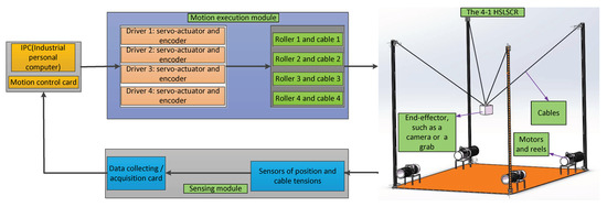
Figure 1.
The composition diagram of the investigated 4-1HSLSCR.
It is also worthwhile mentioning that the tension of the catenary cable, contrary to a straight cable, is not constant along the profile of the catenary cable. In more detail, the cable tension Ti at the terminal point can be defined as Ti= [Hicosθi Hisinθi Hitanγi]T. θi is the angle between the x-axis of the local cable frame and x-axis of the base reference frame; thus, Vi = Hitanγi. The cable tension Ti is decomposed into the three directions of the base reference frame at the terminal point P, and the dynamic equation of the 4-1HSLSCRs with a high speed and long-span cables, using the Newton method, can be expressed according to the following equation:
For simplicity, Eq. (5) can be expressed as follows:
where mp is the mass of the end-effector; is the total mass of the four cables; is the horizontal components of the four cable tensions at the last node P; is the gravitational force of cables; is the gravitational force of the end-effector; is the external forces; is the acceleration of the end-effector; is the structure matrix of the 4-1HSLSCRs; and (i = 1, 2, 3, 4).
Now, Eq. (6) can be expressed in a simpler matrix form as follows:
where and T = [T1, T2, T3, T4]T is the vector consisting of the four cable tensions.
It should be pointed that the dynamic stability of the 4-1HSLSCRs will be proposed based on the position influence factor, cable tension influence factor and the velocity influence factor with dynamic equation of the robots. One important difference is that the qualitative relationship between the stability of the cable robots and the minimum cable tensions was discussed with the static equilibrium in ref. [25].
As mentioned above, the cables have unilateral driving properties so that the 4-1HSLSCRs must be actuated redundantly. Therefore, there must be infinite solutions to the cable tension T, and, according to matrix theory, the vector H can be obtained according to the following equation:
where is the minimum-norm least squares solution to the vector H; is the homogeneous solution; is the kernel of the matrix J; and λ is an arbitrary scalar for the investigated 4-1HSLSCRs.
Moreover, the cable tension can be obtained through the following formula:
The cable tension T needs to meet the following conditions:
where Ts,min is the lower boundary of the cable tension and Ts,max is the upper boundary of the cable tension.
Apart from the abovementioned, keeping the cables as taut as possible is necessary for the 4-1HSLSCRs to work normally. In other words, it is required in actual practice that the sag-to-span ratio denoted by ri is satisfied with the predetermined condition, which can be defined as follows:
Furthermore, there are four cables for the 4-1HSLSCRs, and thus, substituting Eqs. (8) and (9) into (10) yields the following expression:
Additionally, substituting Eqs. (4), (8) and (9) into (11) yields the following expression:
Then, the combination of Eqs. (12) and (13) leads to the following expression:
where is the lower boundary of the arbitrary scalar λ and
is the upper boundary of the arbitrary scalar λ.
As previously mentioned, the cable tension T may have infinite solutions. Under the given situation, the minimum variance of the cable tension is employed to obtain the unique solution for cable tension while using Eqs. (7) and (14) as the constraints of the optimization. Consequently, the determination of the cable tensionT for the 4-1HSLSCRs is formulated as follows:
where E(T) is the arithmetic mean value of T.
Additionally, the cable tension T can be obtained with the optimization model Eq. (15), and furthermore, the minimum cable tension Tmin can be obtained while the end-effector is located at an arbitrary position of the workspace. It should be pointed out that Tmin being the weakest constraint has an important influence on the stability of 4-1HSLSCRs. It can be obtained according to the following equation:
where Tmin is the smallest component in T.
2.1.2. The Influencing Factors of Dynamic Stability
The authors of [20] investigated the effect of the position of the end-effector and the cable tension on the stability of the camera robots by using a massless linear cable model, and furthermore, they studied the position influencing factor and cable tension influencing factor. Then, a force–position stability measure approach for the camera robot was proposed with these influencing factors, which is in the static sense. It should be noted that the abovementioned influencing factors, however, were proposed based on a massless linear cable model, and thus, the sags of the long-span cables were apparently not considered. The long-span cable sags have an important effect on the abovementioned influencing factors, and therefore, the reader can refer to this work for a comprehensive understanding of the two influencing factors, whereas a brief overview is presented in this section. Referring to the definition of each symbol in [20], the position of the end-effector within the workspace is denoted by P; the vertical midline of the workspace is denoted by a; the intersection of the vertical midline and the horizontal plane where the specified position is located is denoted by Q; and the top position of the vertical midline is denoted by M. In this condition, two position influencing factors, and which are related to the position of the end-effector of the 4-1HSLSCR, are proposed and defined as:
where is the position of the end-effector of the 4-1HSLSCR; and , and are the angles between the catenary cable that has the minimum cable tension and is in the horizontal plane while the end-effector is located at the positions of P, Q and M, respectively.
Apart from the abovementioned position influencing factors for the stability of the 4-1HSLSCRs, two cable tension influencing factors, and , which are related to the position of the end-effector and the cable tension of the 4-1HSLSCRs, are proposed, and they can be expressed as:
where , and are the minimum cable tensions while the end-effector of the 4-1HSLSCR is located at the position P, Q and M, respectively.
2.2. The Velocity Influence Function
Additionally, the velocity of the end-effector also has a crucial influence on the stability of the 4-1HSLSCRs. Therefore, this section deliberately emphasizes the effects of the velocity of the end-effector on the stability of the 4-1HSLSCRs. In this regard, a function representing these effects, which is denoted by , is constructed at a later stage.
It should be pointed that with respect to a given position of the end-effector, the end-effector may possess different velocities. Nevertheless, the stability of the 4-1HSLSCRs while the end-effector locates at the given position, through the dual relationship between the velocity of a robot and its stability, is strongest when the velocity of the end-effector is equal to zero. Therefore, for a certain position of the end-effector, the robots are seen as the most stable while . Furthermore, the stability of the 4-1HSLSCRs at the present position with other velocities is lower, and indeed, the stability is the weakest at the present position with the maximum velocity. Meanwhile, in order to employ the interval [0, 1] to measure the stability of the 4-1HSLSCR, the range of the velocity influence function must be the interval [0, 1].
Based upon the analysis and discussion above, the velocity influence function must possess the following three properties:
(1) The range of the velocity influence function is the interval [0, 1], which can be employed to measure the stability of the 4-1HSLSCR.
(2) The stability of the 4-1HSLSCR at the present position becomes weaker with the increase in the velocity of the end-effector.
(3) The present position is assumed to be , and moreover, two extreme cases should be discussed: (i) when the end-effector of the 4-1HSLSCR is located at the present position with a velocity of zero, the 4-1HSLSCR is the most stable, and indeed, the stability measurement does not consider the effect of the velocity on the stability of the 4-1HSLSCR; (ii) when the end-effector of the 4-1HSLSCR is located at the present position with the maximum possible velocity, the 4-1HSLSCR has the weakest stability, and therefore, the stability of the 4-1HSLSCR at the position with the maximum velocity is 0. It should also be noted that the stability of the 4-1HSLSCR at other velocities falls somewhere between the two extremes.
3. Dynamic Stability Measurement Method
The 4-1HSLSCRs employ their flexible cables as the drive system, which leads to the low stability of the motions for the robots. Moreover, 4-1HSLSCRs become unstable when the equilibrium condition of the robot is disturbed by external disturbances during the movement. Therefore, the stability of the 4-1HSLSCR indicates the ability to resist external disturbances in the weakest constraint direction and to keep the end-effector in an equilibrium condition while the external disturbances occur during movement. The dynamic stability of the 4-1HSLSCRs mainly depends on the position and the velocity of the end-effector, as well as the cable tension. For this reason, a dynamic stability measurement method is proposed for 4-1HSLSCRs that have a high speed and long-span cables. Moreover, compared to [20], the innovation of this paper lies in the following two aspects: Firstly, for 4-1HSLSCRs, the velocity of the end-effector is bound to affect the stability of the robot. In this regard, the stability of the 4-1HSLSCR is not only related to the position of the end-effector and the cable tension in the weakest direction, but also related to the motion state of the end-effector. Secondly, compared with the straight line cables used in [20], the long-span catenary cables have an important influence on the cable tension, which further affects the stability of the 4-1HSLSCR. Therefore, the effect of the influence mechanism of the position and the velocity of the end-effector, as well as the cable tension in the weakest constraint direction, on the stability of 4-1HSLSCRs is investigated, and moreover, the dynamic stability measurement method based on the position and cable tension factors, as well as the attitude influence function, is defined as:
where is the stability measurement index when the effects of the velocity on the stability of the camera robot are not considered [20], and p1, p2, q1 and q2 are weight coefficients. It should be noted that the range of , generally speaking, lays between 0 and 1.
As mentioned in the previous description in Section 2.2, the range of the velocity influence function consists of the interval from 0 to 1. Therefore, the values of the dynamic stability measurement index are also the interval from 0 to 1, as was described in Section 1, and the dynamic stability measurement index, which is based on the position, cable tension and velocity factors of the end-effector, measures the dynamic stability of the 4-1HSLSCRs with the interval [0, 1].
It should be pointed out that the dynamic stability of 4-1HSLSCRs is closely related to the kinetic energy of the robots. Therefore, is deliberately chosen to depict the crucial influence of the velocity of the end-effector on the stability of the 4-1HSLSCR. Note that denotes the present end-effector velocity for the 4-1HSLSCRs, whereas denotes the maximum extreme velocity, which means that the 4-1HSLSCRs become unstable with the maximum extreme velocity. This situation should be avoided in practical applications. Note that the velocity influence function is written explicitly as a function of the square of the velocity of the end-effector to provide mathematical insight into the significant relationship between the proposed dynamic stability and the kinetic energy of the 4-1HSLSCRs. According to the kinetic energy equation, it can be seen that the proposed velocity influence function describes the ratio of the kinetic energy between the current motion state and instability state of the end-effector for the 4-1HSLSCRs.
As was stated in Section 2.2., the velocity influence function is required to obtain the proposed three properties. Therefore, the proof that the selected velocity influence function obtains the proposed three properties is given.
Proof:
(1). , . Therefore, the selected velocity influence function meets the requirements of property (1) presented in Section 2.2.
(2). The maximum velocity of the 4-1HSLSCR, , is the constant of the selected 4-1HSLSCR; meanwhile, an increase in the present velocity leads to a corresponding increase in . The values of the selected function decrease with the increase in the velocity of the end-effector of the 4-1HSLSCR. Therefore, the selected function meets the requirements of property (2) presented in Section 2.2.
(3). The selected velocity influence function is equal to 1 when the velocity of the end-effector of the 4-1HSLSCR is equal to zero, and therefore, the dynamic stability of the 4-1HSLSCR is defined as ; the velocity of the end-effector is equal to , and therefore, the selected velocity influence function is equal to 0, leading to . Hence, the selected velocity influence function meets the requirements of property (3) presented in Section 2.2. □
From the above discussion, it can be concluded that the selected velocity influence function satisfies the requirements of all properties. Thus, it can be used to describe the effects of the velocity of the end-effector on the dynamic stability of 4-1HSLSCRs.
4. Dynamic Stability Sensitivity Analysis Method
As mentioned before, the dynamic stability measurement method investigated in Section 3 demonstrated that the position and the velocity of the end-effector, as well as the cable tension, have significant effects on the dynamic stability of 4-1HSLSCRs. As a result, this section mainly focuses on the effect of the influencing degree of these factors on the dynamic stability of 4-1HSLSCRs. It can be seen from Eq. (21) that the stability mechanism of 4-1HSLSCRs is extremely complex and is affected by a considerable number of factors, for example, the position and the velocity of the end-effector, as well as the cable tension. Additionally, the importance of these influencing factors on the dynamic stability of the 4-1HSLSCRs can be evaluated through a sensitivity analysis. The dynamic stability sensitivity analysis of the 4-1HSLSCRs is used to quantitatively investigate the influencing degree of the influencing factors on the stability of a 4-1HSLSCR. The greater sensitivity of an influencing factor on the stability for the 4-1HSLSCRs, the greater influence on the stability, and vice versa. Therefore, through this stability sensitivity analysis, we can identify the influencing factors that have a large influence on the stability. As a result, a dynamic stability sensitivity analysis method for 4-1HSLSCRs is developed in this section using a grey relational analysis. The most sensitive factor among the stability influencing factors can be identified and prioritized. Additionally, with this foundation, the most sensitive dynamic stability influencing factors can be accurately controlled in 4-1HSLSCRs to achieve a more stable operation.
The grey relational analysis uses curves formed by the reference sequence and the comparison sequences to determine the otherness and proximity between them [42,43]. For these reasons, the grey relational degree, in the present paper, is employed to depict the correlation degree between the dynamic stability sequences and influencing factor sequences. Moreover, the instability of the 4-1HSLSCRs results from a variety of factors. The main factors and secondary factors, and the maximum and minimum influencing factors for the stability of the 4-1HSLSCRs, can be accurately identified with a grey relational analysis and grey correlation degree, respectively. Therefore, a grey relational dynamic stability sensitivity analysis method for 4-1HSLSCRs is proposed in this section.
4.1. Determination of the Stability and Influencing Factor Sequences
According to the grey correlation theory, the numerical values of the dynamic stability of the 4-1HSLSCRs are set as the reference sequence, whereas the eight influencing factors (displacement component of the x-axis, y-axis and z-axis; the end-effector velocity; and the four cable tensions) are set as the comparison sequence. Suppose the reference and comparable sequences are denoted as and , respectively, where i indicates the number of the selected comparison sequences composed of the eight influencing factors, and meanwhile, k is the changing number of the dynamic stability influencing factors and the dynamic stability of the 4-1HSLSCRs in this paper. Therefore, the whole sequence matrix consisting of the two crucial sequences can be defined as follows:
4.2. Normalization of the Sequence Matrices
In general, the raw data of the dynamic stability reference sequence and the influencing factor comparison sequence may differ from the others in terms of their range and their measure units, and thus, the influence of some factors may be neglected. Note that this leads to an incomparable condition and incorrect conclusion. Hence, the main procedure of the grey relational analysis is, firstly, a normalization treatment used on the initial data of the sequence matrices to obtain the grey correlation grades. Furthermore, these sequences can be transformed with this formula:
4.3. Grey Correlation Coefficient
After the normalization treatment for the sequence matrices, the absolute difference between the dynamic stability reference and each influencing factor comparison sequence, denoted by , can be obtained. Moreover, the maximum difference denoted by and the minimum difference denoted by can be obtained. Therefore, the grey relation coefficients can be obtained as follows:
where is the distinguishing coefficient, being a positive number which is less than 1, and it is generally chosen as 0.5 [44,45]. The distinguishing coefficients are set as 0.5 and 0.6 to explain the effects of the distinguishing coefficient on the stability sensitivity of the 4-1HSLSCRs in this paper.
4.4. Grey Correlation Dynamic Stability Sensitivity Analysis Index
The correlation between the dynamic stability reference sequence and influencing factor comparison sequences can be represented by a grey relational degree. If a certain influencing factor in the comparison sequence is far more critical than other influencing factors to the dynamic stability, the grey correlation degree of this influencing factor will be higher than other grey correlation degrees. Thus, the grey correlation degree, in this paper, can be employed to measure the influence degree of the end-effector position and the end-effector velocity, as well as the cable tension, on the dynamic stability of the 4-1HSLSCR. Main factors and secondary influencing factors, as well as the maximum and minimum influencing factors for the dynamic stability of the 4-1HSLSCRs, can be obtained through the influencing factor correlation degrees. Based on the above, the grey correlation sensitivity analysis method for the dynamic stability of the robots can be measured with the grey correlation degree, and thus, the dynamic stability sensitivity analysis index, after deriving the grey relational coefficients, can be obtained as follows:
5. Simulation Examples and Results
5.1. Camera Robot—A Selected 4-1HSLSCR
A camera robot, which is a 4-1HSLSCR with a camera platform used for aerial panoramic photographing, as shown in Figure 2, is employed to illustrate the proposed dynamic stability measurement approach and grey relational sensitivity analysis method to determine the dynamic stability of the 4-1HSLSCR. The model parameters of the investigated camera robot are set as shown in Table 1.
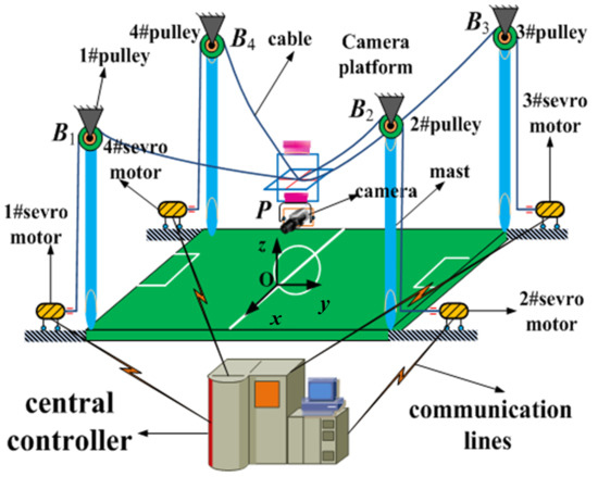
Figure 2.
The investigated camera robot.

Table 1.
Model parameters.
A spatial spiral, as shown in Figure 3, is selected to account for the proposed approaches in this paper, and the selected trajectory is defined as follows:
where R = 10 m; ω = 0.2 πrad/s; and v0 = 0 m/s.

Figure 3.
Spatial spiral trajectory of the camera robot: (a) spatial spiral trajectory; (b) x-component; (c) y-component; (d) z-component.
The selected spatial spiral trajectory and its components for the camera robot are depicted in Figure 3 in more detail. The z-component of the selected spatial spiral trajectory depicted by Eq. (26) is a quadratic function of the time, whereas the velocity in the z-component is a linear function of the time. We should note that the end-effector moves faster on the spatial spiral trajectory, which is different from a uniform spiral.
The dynamic stability of the camera robot is investigated under four situations to investigate the effects of the sags of the long-span cables and the velocity of the end-effector on the dynamic stability of the camera robot. The variable s (s = 1, 2) is employed to express the modeling method of the flexible cables, where s = 1 corresponds to the massless straight line model of the cables and s = 2 corresponds to the catenary model of the cables. The variable t (t = 1, 2) is used to indicate whether the influence of the velocity of the end-effector on the dynamic stability of the camera robot is considered, where t = 1 corresponds to not considering the influence of the end-effector velocity on the dynamic stability, and t = 2 corresponds to considering the influence of the end-effector velocity on the dynamic stability. In more detail, these four situations are shown in Table 2.
Table 2.
Dynamic stability under four conditions.
In the above four cases, the stability of the camera robot under the long-span catenary cables and when considering the influence of the velocity of the end-effector is denoted by ; and the stability of the robot under the massless straight line cables and when not considering the influence of the velocity of the end-effector is represented as . Because the difference between them is the greatest, the stability difference influence index denoted by is used to evaluate the difference between and , and it is defined as follows:
5.2. Results and Discussion
The influence of the moving velocity of the camera robot and the cable modeling methods on the stability are studied in more detail in this section. Firstly, the relationship between the end-effector moving velocity and the stability of the camera robot is further studied by using the simulation analysis. Moreover, the influence curves of the movement velocities of the end-effector on the dynamic stability of the camera robot along the trajectory Eq. (26) with different cable models, namely the massless straight line cables and long-span catenary cables, are shown in Figure 4. Through the comparison, it can be seen that the velocities of the end-effector have a great influence on the dynamic stability under the two kinds of cable modeling methods, and furthermore, the stability of the camera robot obtained with the massless straight line cables is larger than that obtained by the catenary cable model. In particular, because the starting position point has a larger z-coordinate than the ending position point for the selected trajectory, the end-effector located in the upper area of the workspace has a greater stability than the lower area. Therefore, under the same cable model and the same velocity pattern, the dynamic stability of the camera robot at the end of the trajectory, calculated with Eq. (26), is smaller than that at the starting point. As shown in Figure 3a,b, the influence of the velocity of the end-effector on the stability of the camera robot under the straight line cable model and the catenary cable model is depicted, respectively. Note that the average differences of the influence of the end-effector moving velocity on the stability under the straight line cables and catenary cables are as high as 80% and 60%, respectively. Based on the above analysis, we can come to the conclusion that for the camera robot with a high speed and large-span cables, the movement velocity of the end-effector has a crucial effect on the stability of the camera robot.
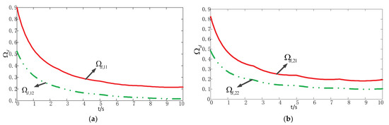
Figure 4.
Stability comparison along the given spatial spiral trajectory when s = 1, t = 1, 2 and s = 2, t = 1, 2: (a) comparison of the stability with s = 1, t = 1 and s = 1, t = 2; (b) comparison of the stability with s = 2, t = 1 and s = 2, t = 2.
Secondly, the influence of the cable modeling methods on the dynamic stability of the camera robot is studied. The influence curves of the cable model methods are shown in Figure 5, which represent the effect of the different moving velocities on the dynamic stability of the camera robot while the camera platform operates along the trajectory calculated using Eq. (26). As can be seen from the four curves in Figure 5, the cable modeling methods have also a certain effect on the dynamic stability of the camera robot, and moreover, the robot stability decreases with the passage of time. This is because with the passage of time, the z-coordinate of the spatial spiral decreases, and meanwhile, the camera platform located in the upper area of the workspace is more stable than the one located in the lower area of the workspace. Therefore, the dynamic stability of the camera robot decreases with time. Note that the dynamic stability is the minimum when the camera platform is located at the end point of the spiral trajectory in Figure 5a due to the velocity influence function of the camera platform at this position. When the camera platform moves at the maximum speed, it is the minimum of the spiral trajectory. Figure 5b shows the curves that do not consider the effects of the moving velocity of the camera platform on the stability of the camera robot, which is the static structural stability proposed in [20], and it can be noted that this is the term in Eq. (19). It can be seen from the figure that under different moving velocities, the average difference of influence of the cable modeling methods on the robot stability reaches 21%. Based on the above analysis, for the camera robot with a high speed and long-span cables, it was found that the cable modeling methods have a crucial effect on the dynamic stability of the camera robot; thus it is necessary to consider the influences of long-span cable sags on the dynamic stability of the camera robot.
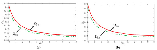
Figure 5.
Comparison of the stability along the given spatial spiral trajectory when s = 1, 2, t = 1 and s = 1, 2, t = 2: (a) comparison of the stability with s = 1, t = 2 and s = 2, t = 2; (b) comparison of the stability with s = 1, t = 1 and s = 2, t = 1.
Thirdly, the influence of the end-effector moving velocity and the cable modeling methods on the stability of the camera robot is investigated. As shown in Figure 6, the influence curves of dynamic stability when considering the moving velocity of the camera platform and cable modeling methods are depicted. It can be seen that the cable modeling mode and moving velocity of the end-effector have a crucial influence on the dynamic stability of the camera robot. There is little difference between the curves in Figure 4a and Figure 6a, and the solid curves at the top in the two figures show the stability of the camera robot with straight line cables when the influence of the moving velocity of the camera platform along the spiral trajectory in space is not considered. The difference lies in the bottom curves depicted by the dotted line. As the difference is small, the curves in Figure 4a and Figure 6a are still similar, and the difference is mainly due to the different influences of the straight line cables and the catenary cables on the stability of the robot. It can be concluded from Figure 6 that whether the moving velocity of the camera robot is considered or not, it has a much greater effect on the robot stability than the different modeling methods of the cables. Moreover, Figure 6b shows the relationship between the stability difference influence index and the time. Note that considering the moving velocity of the camera platform and the catenary cable sags at the same time has a crucial influence on the dynamic stability of the robot, and it should also be noted that its minimum stability difference is as high as 87%.

Figure 6.
Comparison of the stability along the given spatial spiral trajectory when s = 1, t = 1 and s = 2, t = 2: (a) stability comparison; (b) stability difference influence index .
Finally, the influence of the modeling method of the cables on the cable tension is analyzed and studied in this section. A comparison of the cable tensions between catenary cables and straight line cables when the camera platform is manipulated along the spatial spiral trajectory is depicted in Table 3. It should be pointed out that the cable tensions obtained by the two cable models are smooth and continuous, and there is not any impact on the motion of the camera robot. From Table 3 it can be deduced that the cable tension of the catenary cables is about 9 times that of the massless straight line cables. Therefore, the cable sags of the camera robot must be considered.
Table 3.
Cable tensions of the two cable modeling methods along the spatial spiral trajectory.
The values of the dynamic stability of the camera robot along the given trajectory that were calculated with Eq. (26), according to the grey relational sensitivity analysis method for the dynamic stability of the camera robot, are selected as the reference sequence to investigate the dynamic stability sensitivity of the robot. The position and the velocity, as well as the four cable tensions, are taken as the dynamic stability effect factors. Additionally, the numerical values of these dynamic stability effect factors are set as eight comparison sequences. All these sequences are analyzed by preprocessing the data using Eq. (23), and furthermore, the grey relational coefficient can be obtained by Eq. (24). Additionally, the following grey correlation degrees, which are calculated with Eq. (25) while is set as 0.5, are shown in Table 4. It is known that a correlation degree close to 1, according to the grey theory and grey correlation analysis method, means the influence degree of this factor with regard to the dynamic stability of the camera robot is great. It can be seen from Table 4 that the effect of the grey correlation degree of the eight selected influencing factors on the dynamic stability of the camera robot is greater than 0.5, and therefore, this indicates that all of the factors have a crucial influence on the dynamic stability of the robot.
Table 4.
Grey correlation degree of the eight influencing factors on the dynamic stability.
In addition, it should be pointed out that the distinguishing coefficient has an effect on the grey correlation degree between the dynamic stability and its eight influencing factors. Therefore, the distinguishing coefficient is set as 0.5 and 0.6 to explain the influence of the distinguishing coefficient on the dynamic stability sensitivity of the robot, and the grey correlation degree results are shown in Figure 7a,b, respectively. It is worthwhile mentioning that for the different distinguishing coefficients, the influence law of the selected eight influencing factors on the dynamic stability is consistent. In more detail, for the eight selected influencing factors, the importance follows this sequence: cable tension T2 > T4 > T3 > T1 > velocity of the camera platform v > z-direction displacement of the camera platform > x > y. Furthermore, it can be seen that among the eight selected influencing factors, the cable tension has the greatest influence on the dynamic stability of the camera robot, followed by the velocity and position of the camera platform. Therefore, the four cable tensions must be strictly controlled during the operation to improve the stability of the camera robot.
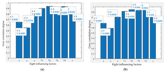
Figure 7.
Grey correlation degree between dynamic stability and eight influencing factors (a) ; (b) .
To summarize, the following conclusions can be drawn from the theoretical and simulation analysis of this paper. For the 4-1HSLSCRs, the self-weights of the cables and the velocity of the end-effector have a crucial influence on the stability and the cable tension of the robots, and it should be pointed that the velocity of the end-effector has a more important influence on the dynamic stability of the 4-1HSLSCRs. Moreover, we must note that the used control strategy is bound to affect the stability influencing factors during the actual motion control process, and therefore, the practical stability and stability optimization of the 4-1HSLSCRs can be obtained with an appropriate and robust control strategy, such as computed torque control [46], adaptive fuzzy sliding mode control [47], etc. The sensitivity analysis of the 4-1HSLSCRs can determine the primary and secondary influencing factors of the dynamic stability, whereas the research results can be employed in the design of a robust motion trajectory and motion control for 4-1HSLSCRs. This will lead to the theoretical and engineering practical value of improving the dynamic stability of 4-1HSLSCRs.
6. Conclusions
Stability is a crucial and significant characteristic of cable robots. It has also been a great concern in cable robots, especially for 4-1HSLSCRs that have a high speed and long-span cables. This paper, as a result, focused on two special problems of dynamic stability measurement and stability sensitivity analysis for 4-1HSLSCRs. The following conclusions can be drawn from the presented analysis results:
(1) This paper discusses the influence mechanism of the position and velocity of the end-effector, as well as the cable tension, with regard to the dynamic stability of 4-1HSLSCRs, and proposes a dynamic stability measurement method for 4-1HSLSCRs with a high speed and long-span cables.
(2) The dynamic stability of the 4-1HSLSCRs is influenced by various factors, and these various influencing factors have different sensitivities. A grey relational analysis can investigate the sensitivity of the influencing factors on the dynamic stability of the 4-1HSLSCRs. The sensitivity analysis model for the dynamic stability of 4-1HSLSCRs, as a result, is established by using the grey relational analysis method.
(3) A camera robot, which is a 4-1HSLSCR with a camera platform that can be used in aerial panoramic photographing, is employed to illustrate the proposed dynamic stability measurement approach and grey relational stability sensitivity analysis method. On the one hand, the dynamic stability measurement simulation proves that the weights and the configurations of the long-span cables and the velocity of the end-effector have great effects on the dynamic stability and the cable tension of the robots. It should be noted that the minimum stability difference when considering the velocity of the camera platform and the catenary cable sags at the same time is as high as 87%. Meanwhile, the cable tension in the catenary cables is about 9 times that of the massless straight line cables. On the other hand, for the eight selected influencing factors, the following sequence can be determined based on importance: cable tension T2 > T4 > T3 > T1 > velocity of the camera platform v > z-direction displacement of the camera platform > x > y. It can be seen that among the eight selected influencing factors, the cable tension has the greatest effect on the dynamic stability of the robots, followed by the velocity and position of the camera platform. Therefore, the four cable tensions must be strictly controlled during its operation to improve the stability of the camera robot.
The investigated 4-1HSLSCR in this work is actually a cable robot with a point-mass end-effector, and as a consequence, the effect of the posture of the end-effector is not considered. It is noted that the posture of the end-effector, however, is bound to affect the stability of the cable robots. Our studies, as a result, will focus on the influencing mechanism of the posture of the end-effector on the stability of cable robots, in addition to verifying the proposed methods and the obtained results of this paper for the improvement of cable robots.
Author Contributions
Conceptualization, P.L.; methodology, P.L.; software, Y.S.; validation, P.L. and X.Q.; formal analysis, Y.S.; investigation, P.L.; resources, H.T.; data curation, X.C.; writing—original draft preparation, P.L.; writing—review and editing, P.L. and X.Q.; supervision, P.L.; project administration, X.Z.; funding acquisition, P.L. and H.T. All authors have read and agreed to the published version of the manuscript.
Funding
This research was funded through the financial support of the National Natural Science Foundation of China (NSFC) under Grant NO. 52174149, the Bilin District Applied Technology Research and Development Projects in 2022 under Grant No. GX2228, and the Key Research and Development Program of Shaanxi Province under Grant NO. 2022GY-241.
Institutional Review Board Statement
Not applicable.
Informed Consent Statement
Not applicable.
Data Availability Statement
The data used to support the findings of this study are available from the corresponding author upon request.
Acknowledgments
This research is supported by the Open Fund of Key Laboratory of Electronic Equipment Structure Design (Ministry of Education) of Xidian University. The authors are grateful to the Guest Editors, Róbert Szabolcsi and Péter Gáspár, as well as the anonymous reviewers for their constructive comments and helpful suggestions that greatly improved the quality of this article.
Conflicts of Interest
The author(s) declare no potential conflicts of interest with respect to the research, authorship and/or publication of this article.
References
- Duan, Q.J.; Duan, X. Workspace Classification and Quantification Calculations of Cable-Driven Parallel Robots. Adv. Mech. Eng. 2014, 6, 358727. [Google Scholar] [CrossRef]
- Tang, L.; Shi, P. Design and analysis of a gait rehabilitation cable robot with pairwise cable arrangement. J. Mech. Sci. Technol. 2021, 35, 3161–3170. [Google Scholar] [CrossRef]
- Rasheed, T.; Long, P.; Caro, S. Wrench-Feasible Workspace of Mobile Cable-Driven Parallel Robots. J. Mech. Robot. 2020, 12, 031009. [Google Scholar] [CrossRef]
- Goodarzi, R.; Korayem, M.H.; Tourajizadeh, H.; Nourizadeh, M. Nonlinear dynamic modeling of a mobile spatial cable-driven robot with flexible cables. Nonlinear Dyn. 2022, 108, 3219–3245. [Google Scholar] [CrossRef]
- Abbasnejad, G.; Tale-Masouleh, M. Optimal wrench-closure configuration of spatial reconfigurable cable-driven parallel robots. Proc. Inst. Mech. Eng. Part C J. Mech. Eng. Sci. 2021, 235, 4049–4056. [Google Scholar] [CrossRef]
- Li, X.M.; Yang, Q.Q.; Song, R. Performance-Based Hybrid Control of a Cable-Driven Upper-Limb Rehabilitation Robot. IEEE Trans. Biomed. Eng. 2021, 68, 1351–1359. [Google Scholar] [CrossRef] [PubMed]
- Wang, Y.L.; Wang, K.Y.; Wang, K.C.; Mo, Z.J. Safety Evaluation and Experimental Study of a New Bionic Muscle Cable-Driven Lower Limb Rehabilitation Robot. Sensors 2020, 20, 7020. [Google Scholar] [CrossRef] [PubMed]
- Tourajizadeh, H.; Yousefzadeh, M.; Khalaji, A.K.; Bamdad, M. Design, Modeling and Control of a Simulator of an Aircraft Maneuver in the Wind Tunnel Using Cable Robot. Int. J. Control Autom. Syst. 2022, 20, 1671–1681. [Google Scholar] [CrossRef]
- Wang, X.G.; Peng, M.J.; Hu, Z.H.; Chen, Y.S.; Lin, Q. Feasibility investigation of large-scale model suspended by cable-driven parallel robot in hypersonic wind tunnel test. Proc. Inst. Mech. Eng. Part G J. Aerosp. Eng. 2017, 231, 2375–2383. [Google Scholar] [CrossRef]
- Li, H.; Yao, R. Optimal Orientation Planning and Control Deviation Estimation on FAST Cable-Driven Parallel Robot. Adv. Mech. Eng. 2014, 6, 716097. [Google Scholar] [CrossRef]
- Yin, J.N.; Jiang, P.; Yao, R. An approximately analytical solution method for the cable-driven parallel robot in FAST. Res. Astron. Astrophys. 2021, 21, 046. [Google Scholar] [CrossRef]
- Li, G.; Ge, R.; Loianno, G. Cooperative Transportation of Cable Suspended Payloads With MAVs Using Monocular Vision and Inertial Sensing. IEEE Robot. Autom. Lett. 2021, 6, 5316–5323. [Google Scholar] [CrossRef]
- Rossonnando, F.; Rosales, C.; Gimenez, J.; Salinas, L.; Soria, C.; Sarcinelli-Filho, M.; Carelli, R. Aerial Load Transportation with Multiple Quadrotors Based on a Kinematic Controller and a Neural SMC Dynamic Compensation. J. Intell. Robot. Syst. 2020, 100, 519–530. [Google Scholar] [CrossRef]
- Xian, B.; Wang, S.; Yang, S. Nonlinear adaptive control for an unmanned aerial payload transportation system: Theory and experimental validation. Nonlinear Dyn. 2019, 98, 1745–1760. [Google Scholar] [CrossRef]
- Tang, X. An Overview of the Development for Cable-Driven Parallel Manipulator. Adv. Mech. Eng. 2014, 6, 823028. [Google Scholar] [CrossRef]
- Qian, S.; Zi, B.; Shang, W.W.; Xu, Q.S. A Review on Cable-driven Parallel Robots. Chin. J. Mech. Eng. 2018, 31, 66. [Google Scholar] [CrossRef]
- Wei, H.L.; Qiu, Y.Y.; Sheng, Y. On the Cable Pseudo-Drag Problem of Cable-Driven Parallel Camera Robots at High Speeds. Robotica 2019, 37, 1695–1709. [Google Scholar] [CrossRef]
- Su, Y.; Qiu, Y.; Liu, P.; Tian, J.; Wang, Q.; Wang, X. Dynamic Modeling, Workspace Analysis and Multi-Objective Structural Optimization of the Large-Span High-Speed Cable-Driven Parallel Camera Robots. Machines 2022, 10, 565. [Google Scholar] [CrossRef]
- Liu, P.; Qiu, Y.; Su, Y. A new hybrid force-position measure approach on the stability for a camera robot. Proc. Inst. Mech. Eng. Part C J. Mech. Eng. Sci. 2016, 230, 2508–2516. [Google Scholar] [CrossRef]
- Liu, P.; Qiu, Y. Approach with a hybrid force-position property to assessing the stability for camera robots. J. Xidian Univ. 2016, 43, 87–93. [Google Scholar] [CrossRef]
- Su, Y.; Qiu, Y.; Liu, P. Optimal Cable Tension Distribution of the High-Speed Redundant Driven camera robots Considering Cable Sag and Inertia Effects. Adv. Mech. Eng. 2014, 6, 729020. [Google Scholar] [CrossRef]
- Korayem, M.H.; Yousefzadeh, M.; Susany, S. Dynamic Modeling and Feedback Linearization Control of Wheeled Mobile Cable-Driven Parallel Robot Considering Cable Sag. Arab. J. Sci. Eng. 2017, 42, 4779–4788. [Google Scholar] [CrossRef]
- Sohrabi, S.; Daniali, H.M.; Fathi, A.R. Dynamic Modeling of Long Span New Material Cable Robot. Trans. Can. Soc. Mech. Eng. 2017, 41, 517–530. [Google Scholar] [CrossRef]
- Behzadipour, S.; Khajepour, A. Stiffness of Cable-based Parallel Manipulators With Application to Stability Analysis. J. Mech. Des. 2005, 128, 303–310. [Google Scholar] [CrossRef]
- Liu, P.; Qiu, Y.; Su, Y.; Chang, J. On the Minimum Cable Tensions for the Cable-Based Parallel Robots. J. Appl. Math. 2014, 2014, 350492. [Google Scholar] [CrossRef]
- Bosscher, P.; Ebert-Uphoff, I. A Stability Measure for Underconstrained Cable-Driven Robots. In Proceedings of the IEEE International Conference on Robotics and Automation, 2004, Proceedings, ICRA ‘04. 2004, New Orleans, LA, USA, 26 April–1 May 2004; Volume 4945, pp. 4943–4949. [Google Scholar]
- Bosscher, P.M. Disturbance Robustness Measures and Wrench-Feasible Workspace Generation Techniques for Cable-Driven Robots; Georgia Institute of Technology: Atlanta, GA, USA, 2004. [Google Scholar]
- Liu, P.; Qiao, X.; Zhang, X. Stability sensitivity for a cable-based coal-gangue picking robot based on grey relational analysis. Int. J. Adv. Robot. Syst. 2021, 18, 17298814211059729. [Google Scholar] [CrossRef]
- Wang, Y.-l.; Wang, K.-y.; Wang, W.-l.; Yin, P.-c.; Han, Z. Appraise and analysis of dynamical stability of cable-driven lower limb rehabilitation training robot. J. Mech. Sci. Technol. 2019, 33, 5461–5472. [Google Scholar] [CrossRef]
- Liu, S.; Lin, Y. Introduction to Grey Systems Theory. In Grey Systems; Springer: Berlin/Heidelberg, Germany, 2010; pp. 1–18. [Google Scholar]
- Ju-Long, D. Control problems of grey systems. Syst. Control Lett. 1982, 1, 288–294. [Google Scholar] [CrossRef]
- Liu, S.; Forrest, J.Y.L. Grey Systems: Theory and Applications; Springer Science & Business Media: Berlin/Heidelberg, Germany, 2010. [Google Scholar]
- Liu, S.f.; Xie, N.m.; Forrest, J. Novel models of grey relational analysis based on visual angle of similarity and nearness. Grey Syst. Theory Appl. 2011, 1, 8–18. [Google Scholar] [CrossRef]
- Patil, A.; Walke Gaurish, A.; Mahesh, G. Grey relation analysis methodology and its application. Res. Rev. Int. J. Multidiscip. 2019, 4, 409–411. [Google Scholar]
- He, X.Y.; Li, L.P.; Liu, X.J.; Wu, Y.S.; Mei, S.J.; Zhang, Z. Using grey relational analysis to analyze influential factor of hand, foot and mouth disease in Shenzhen. Grey Syst.-Theory Appl. 2019, 9, 197–206. [Google Scholar] [CrossRef]
- Zhang, C.X.; Duan, L.Z.; Liu, H.Y.; Zhang, Y.R.; Yin, L.L.; Lu, Q.; Duan, G.N. Identifying the Influencing Factors of Patient’s Attitude to Medical Service Price by Combing Grey Relational Theory with CMH Statistical Analysis. J. Grey Syst. 2020, 32, 80–95. [Google Scholar]
- Duran, E.; Duran, B.U.; Akay, D.; Boran, F.E. Grey relational analysis between Turkey’s macroeconomic indicators and domestic savings. Grey Syst.-Theory Appl. 2017, 7, 45–59. [Google Scholar] [CrossRef]
- Chen, X.D.; Pei, D.S.; Li, L.P. Grey relation between main meteorological factors and mortality. Grey Syst.-Theory Appl. 2019, 9, 185–196. [Google Scholar] [CrossRef]
- Chang, S.; Huang, F.; Zhao, J.J.; Zhang, Y. Identifying Influential Climate Factors of Land Surface Phenology Changes in Songnen Plain of China Using Grid-based Grey Relational Analysis. J. Grey Syst. 2018, 30, 18–33. [Google Scholar]
- Yang, L.; Xie, N.M. Evaluation of provincial integration degree of “internet plus industry” based on matrix grey relational analysis Case of China 2014–2016. Grey Syst.-Theory Appl. 2019, 9, 31–44. [Google Scholar] [CrossRef]
- Liu, P.; Ma, H. On the Stability for a Cable-Driven Parallel Robot While Considering the Cable Sag Effects. In Proceedings of the 2016 13th International Conference on Ubiquitous Robots and Ambient Intelligence (URAI), Xi’an, China, 19–22 August 2016; pp. 538–543. [Google Scholar]
- Kuo, T. A Review of Some Modified Grey Relational Analysis Models. J. Grey Syst. 2017, 29, 70–77. [Google Scholar]
- Liu, H.; Liu, Q.; Hu, Y. Evaluating Risks of Mergers & Acquisitions by Grey Relational Analysis Based on Interval-Valued Intuitionistic Fuzzy Information. Math. Probl. Eng. 2019, 2019, 3728029. [Google Scholar] [CrossRef]
- Huang, C.-Y.; Lin, Y.-C.; Lu, Y.-C.; Chen, C.-I. Application of Grey Relational Analysis to Predict Dementia Tendency by Cognitive Function, Sleep Disturbances, and Health Conditions of Diabetic Patients. Brain Sci. 2022, 12, 1642. [Google Scholar] [CrossRef]
- Tsolas, I.E. Financial Performance Assessment of Construction Firms by Means of RAM-Based Composite Indicators. Mathematics 2020, 8, 1347. [Google Scholar] [CrossRef]
- Begey, J.; Cuvillon, L.; Lesellier, M.; Gouttefarde, M.; Gangloff, J. Dynamic Control of Parallel Robots Driven by Flexible Cables and Actuated by Position-Controlled Winches. IEEE Trans. Robot. 2019, 35, 286–293. [Google Scholar] [CrossRef]
- Llopis-Albert, C.; Rubio, F.; Valero, F. Modelling an Industrial Robot and Its Impact on Productivity. Mathematics 2021, 9, 769. [Google Scholar] [CrossRef]
Publisher’s Note: MDPI stays neutral with regard to jurisdictional claims in published maps and institutional affiliations. |
© 2022 by the authors. Licensee MDPI, Basel, Switzerland. This article is an open access article distributed under the terms and conditions of the Creative Commons Attribution (CC BY) license (https://creativecommons.org/licenses/by/4.0/).