Article

Slow–Fast Dynamics Behaviors under the Comprehensive Effect of Rest Spike Bistability and Timescale Difference in a Filippov Slow–Fast Modified Chua’s Circuit Model

1
Faculty of Civil Engineering and Mechanics, Jiangsu University, Zhenjiang 212013, China
2
Faculty of Mathematics and Statistics, Yancheng Teachers University, Yancheng 224002, China
3
School of Aeronautics and Astronautics, Sichuan University, Chengdu 610065, China
*
Author to whom correspondence should be addressed.
Mathematics 2022, 10(23), 4606; https://doi.org/10.3390/math10234606
Submission received: 23 October 2022 / Revised: 29 November 2022 / Accepted: 1 December 2022 / Published: 5 December 2022
(This article belongs to the Special Issue Modeling and Analysis in Dynamical Systems and Bistability)

Abstract

:
Since the famous slow–fast dynamical system referred to as the Hodgkin–Huxley model was proposed to describe the threshold behaviors of neuronal axons, the study of various slow–fast dynamical behaviors and their generation mechanisms has remained a popular topic in modern nonlinear science. The primary purpose of this paper is to introduce a novel transition route induced by the comprehensive effect of special rest spike bistability and timescale difference rather than a common bifurcation via a modified Chua’s circuit model with an external low-frequency excitation. In this paper, we attempt to explain the dynamical mechanism behind this novel transition route through quantitative calculations and qualitative analyses of the nonsmooth dynamics on the discontinuity boundary. Our work shows that the whole system responses may tend to be various and complicated when this transition route is triggered, exhibiting rich slow–fast dynamics behaviors even with a very slight change in excitation frequency, which is described well by using Poincaré maps in numerical simulations.

1. Introduction

In the past decades, many research groups and scholars have studied slow–fast dynamical systems via experiments and computations based on extensive applications across many practical problems. For instance, neuronal activities and neural networks [1,2,3], calcium-ion oscillations in cells [4,5], catalytic oxidation reactions [6,7], and other applications [8,9,10].
Such systems frequently behave in complicated nonlinear phenomena characterized by various slow–fast dynamic behaviors such as relaxation oscillations, canard phenomena, bursting oscillations and mixed-mode oscillations. For more details, we suggest readers refer to the references [10,11] in addition to the references therein. In particular, bursting oscillations are generally more complicated and varied in oscillation patterns and generation mechanisms than the other three, and receive much more attention from scholars. In bursting oscillations, the waveform often presents periodic alternations between a cluster of spiking pattern (SP) and a period of quiescent state (QS). A general and powerful approach to deal with the mechanism of bursting phenomena in a slow–fast dynamical system is based on phase reduction and bifurcation theories [12,13]. Such methodology, i.e., the so-called slow–fast decomposition analysis, mainly consists of two steps: firstly, dividing the whole system into a fast subsystem and a slow subsystem via the timescale separation of state variables; secondly, utilizing the attractor structures and their bifurcations of the fast subsystem to explain the generation mechanism of potential bursting oscillations. Based on this method, bursting phenomena and the underlying generation mechanisms are well understood by employing dynamics of the fast subsystems. Relatively complete bursting patterns have been listed by Izhikevich [14] via slow–fast decomposition. More importantly, Izhikevich also provides a widely adopted classification method for bursting phenomena, by which one bursting oscillation can be named according to the two important bifurcations leading to transitions between QSs and the following SPs. For instance, “subcritical–Hopf/LPC” bursting means that the following dynamical generation mechanism can explain this bursting phenomenon: the trajectory will behave in SPs after it passes through a subcritical-Hopf bifurcation point and may enter into the following QS via the bifurcation LPC (fold bifurcation of limit cycles).
Since the dynamic features of the fast subsystems play the leading role in bursting oscillations, many researchers have paid increasing attention to the complicated structures existing in the fast subsystems, such as bistability and nonsmooth factors. Moreover, novel bursting patterns in addition to the related generation mechanisms have been explored in experiments and numerical computations in succession.
Bistability, referring to two coexisting attractors in a fixed parameter range, represents a common dynamics structure in nonlinear dynamical systems, and mounting evidence suggests that this geometric structure is a key factor (but not necessary) in the presence of bursting oscillations [2,14,15,16]. Two coexisting stable equilibria have been analytically investigated to be the principal reason of winner-take-all behavior in competition models [2,17], or the binocular rivalry in the so-called Levelt’s propositions [18]. Another bistability structure, namely rest spike bistability consisting of a stable limit cycle and a stable equilibrium separated by a saddle, has been studied as the core structure for slow spiking and bursting phenomena in the family of Morris–Lecar models [19]. The mixed bursting oscillation is a novel bursting form recently observed in a study by Ref. [20], where the trajectory can perform different SP patterns in a complete periodic motion. Duan et al. point out that such a special bursting pattern can be explained by bistability structures in the fast subsystem [21]. In continuous slow–fast dynamical systems, the slow–fast dynamic behaviors as well as the generation mechanisms are well understood based on slow–fast decomposition and the relatively well-developed conventional dynamics theories [22].
Discontinuity boundaries will exist in the fast subsystems where some nonsmooth events are involved, on which nonconventional dynamic behaviors may appear and participate in the dynamical evolution process of bursting oscillations. In nonlinear rotary drilling systems, friction induced by bit-rock interaction laws can cause the vector fields to become discontinuous, leading to the unique nonsmooth bursting patterns characterized by stick–slip motions [23,24,25]. Similar nonsmooth bursting patterns can also be observed when adopting a threshold control strategy in the Hindmarsh–Rose neuronal model [26]. On the other hand, owing to the unique advantages of nonsmoothness, almost all of the artificial neuron models are designed to be discontinuous [27].
In the slow–fast dynamical systems with discontinuous vector fields, complicated structures may be observed in the slow–fast dynamic behaviors when they interact with discontinuity boundaries, and the traditional dynamics and bifurcation theories may be useless to the understanding of those slow–fast dynamics behaviors. Fortunately, owing to the successful application of differential inclusion theory [28], nonconventional dynamics and bifurcation theories are developing rapidly (more details can be seen in [29] as well as the references therein). Riding on the nonconventional dynamics theories, scholars have proved that many nonconventional bifurcations may also affect the transition mechanisms of slow–fast dynamic behaviors, for instance, nonsmooth fold bifurcation and boundary homoclinic bifurcation can also cause the alternations between QSs and SPs [30,31,32]. Sliding bifurcations lead to unique sliding structures in SPs, although they do not result in transitions between QSs and SPs [33]. In [34], it was proved that boundary homoclinic bifurcation is a high codimension nonconventional bifurcation, which may result in different nonsmooth bursting patterns under different local structures of pseudo-equilibrium.
Almost all the above papers related to bursting phenomena indicate that bifurcations seem to be the only explanation for alternations between QSs and SPs. Recently, a different viewpoint was provided in the works [35,36,37] via proposal of the novel bursting mode referred to as pulse-shaped explosion, which can be attributed to the asymptotic behavior of vector field rather than bifurcations of attractors. Hastings et al. also pointed out that the saddle point and ghost attractor are the two essential elements leading to the non-bifurcation-induced transition in long-term ecological understanding [38]. This indicates that the related works regarding bursting oscillations also need to consider not only potential bifurcations but, more importantly, special flow structures in the fast subsystems.
In previous works related to bursting oscillations, the transition mechanism of bursting phenomena can be roughly classified into the following two types.
  • The bifurcation-induced transition mechanism, which means that the bifurcation structures of attractors in the fast subsystems can explain the transitions in bursting oscillations very well.
  • Non-bifurcation-induced transition mechanism, which means that the transitions in bursting oscillations can only be attributed to the unique manifold structures rather than to the bifurcation structures.
The bifurcation-induced transition mechanism in continuous (or discontinuous) slow–fast dynamical systems can be regarded as the replay of dynamics structures of bifurcations, which can be predicted well via bifurcation analyses of the fast subsystems, and the related achievements are plentiful and substantial. However, for the non-bifurcation-induced transition mechanism, there is not yet a useful research method, and the research also is relatively lag. Accordingly, further exploration of non-bifurcation-induced transition mechanism is important and meaningful to the comprehensive understanding of bursting phenomena in the slow–fast dynamics theory.
In the recent works by [30,39] involving Filippov slow–fast dynamical systems, unique nonsmooth rest spike bistability consisting of a stable nonsmooth cycle and the inner stable pseudo-equilibrium point is proved as the core structure of bursting patterns. Specifically, the alternation from the spike attractor (stable cycle) to the rest attractor (inner equilibrium) is not caused by bifurcations in the fast subsystems, thus indicating the occurrence of a non-bifurcation-induced transition. However, unfortunately, the underlying dynamics mechanism still needs to be clarified. Based on this, we will present further discussion of such non-bifurcation-induced transition structure in this paper by establishing a Filippov modified Chua’s circuit model with an external low–frequency excitation. Furthermore, we try to analyze the dynamics generation mechanism and the induced slow–fast dynamics behaviors, especially the influence on whole system responses, through quantitative calculations and qualitative analyses.
The rest of this paper is organized as follows. Section 2 presents a 3D Filippov slow–fast dynamical system by establishing a Filippov modified Chua’s circuit with an external low-frequency excitation. In Section 3, nonsmooth singularities are analyzed by employing nonconventional dynamics theory. Various slow–fast dynamics behaviors as well as the generation mechanisms are presented in Section 4 via numerical simulations. We draw some conclusions and discussions in Section 5.

2. Mathematical Model

The typical Chua’s circuit and modifications have been taken as examples in many studies of slow–fast dynamics via experiments or numerical simulations. To name but a few, canards and chaotic bursting were reproduced in memristor-based Chua’s circuit [40]; Marszalek and Trzaska analyzed mixed-mode oscillations and relaxations in slow–fast modified Chua’s circuit models with autonomous vector fields [41]. Particularly, those modified Chua’s circuits with low–frequency excitations are also employed to investigate various bursting oscillations and the generation mechanisms [24,25,26,42].
Here, we consider one modified Chua’s circuit by introducing a current source, as shown in Figure 1a. Such a circuit system consists of two capacitances C 1 , 2 , one inductance L, one constant resistance R, one sinusoidal current source i S = I m sin ( ω t ) and one nonlinear resistance R N . According to the Kirchhoff Law, the state equations can be expressed in the 3D ordinary differential equations
C 1 d u 1 d t = u 2 u 1 R g u 1 + i S , C 2 d u 2 d t = i L + u 1 u 2 R , L d i L d t = u 2 ,
where R N is designed as a nonlinear resistance possessing a piece-wise smooth voltage–current characteristic via introducing one comparator, as shown in Figure 1b. Then, the voltage–current characteristic can be written as
i N = g ( u 1 ) = R 12 ( R 15 + R 16 ) + R 13 R 16 R 12 R 15 R 18 u 1 R 10 R 16 ( R 7 + R 6 ) 100 R 6 R 8 R 11 R 18 u 1 3 + ( R 1 + R 2 ) R 16 R 1 R 4 R 18 E s a t sgn ( u 1 ) .
It can be found that u 1 = 0 defines a discontinuity boundary, labeled as Σ , which means that the vector field of system (1) then is piece-wise smooth.
Using the following transformations τ = t R C 2 , x = u 1 E s a t , y = u 2 E s a t , z = R i L E s a t , α = C 2 C 1 , a = ( R 12 R 15 + R 12 R 16 + R 13 R 16 ) R R 12 R 15 R 18 , b = R 10 R 16 ( R 7 + R 6 ) R E s a t 2 100 R 6 R 8 R 11 R 18 , δ = α ( R 1 + R 2 ) R 16 R R 1 R 4 R 18 , A = R I m α E s a t , Ω = ω R C 2 and η = R 2 C 2 L , we can rewrite system (1) into the dimensionless form
x ˙ = α y x f ( x ) + δ sgn H ( X ) + A sin ( Ω τ ) , y ˙ = x y + z , z ˙ = η y ,
where · = d d τ , f ( x ) = a x + b x 3 , X = x y z T , α , b, A, Ω , η are positive while a, δ are negative, H ( X ) : = x = 0 represents the discontinuity boundary Σ .
With the assumption that Ω is small enough, i.e., 0 < Ω 1 , then there exists an order gap between the rates of traditional variables (x, y and z) and the whole excitation, admitting that the system (3) may perform slow–fast dynamics behaviors. However, there is no apparent fast variables and slow variables in (3), indicating that the classical slow–fast decomposition method cannot be directly applied to (3) to explain the potential slow–fast dynamics behaviors such as bursting oscillations since the division of the slow subsystem and the fast subsystem in (3) is the first requirement for the application of this method. In order to apply the classical slow–fast decomposition method to deal with the potential slow–fast dynamics behaviors in (3), we now introduce the following rise–dimension method to realize the timescale separation in (3).
Actually, A sin ( Ω τ ) , A cos ( Ω τ ) = w ( τ ) , v ( τ ) can be described by a simple planar–linear system ( w ˙ = Ω v ; v ˙ = Ω w ) with the initial condition w ( 0 ) = A sin ( 0 ) , v ( 0 ) = A cos ( 0 ) = ( 0 , A ) . Therefrom, system (3) then is equivalent to a 3D Filippov fast subsystem (FS) controlled by a 2D smooth slow subsystem (SS), respectively, expressed as
x ˙ = α y x f ( x ) + δ sgn H ( X ) + w , y ˙ = x y + z , z ˙ = η y , ( FS )
and
w ˙ = Ω v , v ˙ = Ω w . ( SS )
We then have transformed (3) into the standard form represented by a 5D autonomous Filippov slow–fast dynamical system that embodies three fast variables (x, y and z) and two slow variables (w and v). Although the rise–dimension method seems to increase the difficulty in the analysis of (3), it should be pointed out that only the slow variable w appears in the fast subsystem (4), indicating that the dynamics structures of the fast subsystem only can be affected by w. As a consequence, the classical slow–fast decomposition method can be directly employed to explain the generation mechanism of slow–fast dynamics behaviors in (3) just via regarding the slow variable w as a bifurcation parameter in (4). Meanwhile, the rise–dimension method also demonstrates that the generalized slow–fast analysis method proposed in [42] is feasible mathematically and logically.
When attractors of the fast subsystem come into contact with the discontinuity boundary Σ , unique nonsmooth dynamics such as sliding bifurcations and boundary equilibrium bifurcations may appear and affect the responses of whole system (3). In the following section, we mainly focus on the analyses of nonsmooth dynamics on Σ .

3. Nonsmooth Dynamics Analyses

Note that the discontinuity boundary Σ divides the whole phase space R = { X | ( x , y , z ) } into two subregions R + = { X | ( x , y , z ) , ( x > 0 ) } and R = { X | ( x , y , z ) , ( x < 0 ) } , where two 3D smooth subsystems, denoted by S + ( x > 0 ) and S ( x < 0 ) , can be observed in the two subregions, and the vector fields are, respectively, labeled as F + ( x > 0 ) and F ( x < 0 ) . Let X Σ ( 0 , y Σ , z Σ ; w ) be a point on Σ , by using the two Lie derivatives L F + H = H , F + and L F H = H , F ( H = H ( X Σ ) X Σ , · , · denotes the vector inner product), the discontinuity boundary Σ can be divided into different regions [43].
If L F + H · L F H > 0 , i.e., F + and F have the same direction on Σ at X Σ , then we can define the two so-called sewing regions
Σ + = { X Σ | α y Σ + w δ > 0 , α y Σ + w + δ > 0 } , Σ = { X Σ | α y Σ + w δ < 0 , α y Σ + w + δ < 0 } ,
where the trajectory will cross through the discontinuity boundary without sliding motion when it interacts with Σ in Σ + (or Σ ).
If L F + H · L F H < 0 , L F + H < 0 and L F H > 0 , i.e., both F + and F point to Σ at X Σ , then we can define a so-called sliding region
Σ S = { X Σ | α y Σ + w δ > 0 , α y Σ + w + δ < 0 } ,
where the trajectory will enter into Σ and behave in the special sliding motion when it interacts with Σ S .
In particular, there are two so-called sliding boundaries between the two sewing regions (6) and the sliding region (7), which can be defined by L F + H = 0 and L F H = 0 , respectively, expressed by
Σ S + = { X Σ | α y Σ + w + δ = 0 } , Σ S = { X Σ | α y Σ + w δ = 0 } .
Meanwhile, one 2D sliding vector field located in Σ S can be derived as F S = F + F + 2 + Q F + F 2 by introducing a scalar Q [ 1 , 1 ] via the Utkin’s equivalent control method, corresponding to a linear-planar system
y ˙ Σ = y Σ + z Σ , z ˙ Σ = η y Σ .
Besides the two 3D smooth subsystems S + and S , one may find that the Filippov fast subsystem (4) also has one 2D sliding subsystem (9) in Σ S . Modulated by the slow variable w, attractors such as equilibria and cycles of smooth subsystems may collide with a sliding boundary in (8), behaving in nonconventional bifurcations. In other words, nonconventional bifurcations in (4) generally occur on sliding boundaries. We now turn to discuss the equilibria and their stabilities as well as nonconventional bifurcations.

3.1. Equilibria and the Stabilities

Since the system (3) is Z 2 symmetrical, the equilibrium points of the fast subsystem (4) can be written as X 0 = ( x 0 , 0 , x 0 ; w ) . The equilibria in Filippov dynamical systems can be classified into the following four types: admissible equilibrium, pseudo equilibrium, boundary equilibrium and virtual equilibrium [29]. Furthermore, the first three types of equilibria really exist in the state space. In contrast, the last type of equilibrium does not exist in the state space and should be useless for understanding the slow–fast dynamics behaviors. Based on the fact that the Filippov fast subsystem (4) consists of two 3D smooth subsystems S + , S as well as one 2D sliding subsystem, we then have the following definition for the equilibria that really exist in the fast subsystem (4).
Definition 1.
The real equilibria of the fast subsystem (4) can be classified into the three types:
1. 
if F + ( X 0 ) = 0 and x 0 > 0 ( F ( X 0 ) = 0 and x 0 < 0 ), X 0 is a so-called admissible equilibrium (AE), and x 0 is restricted by w = x 0 + f ( x 0 ) δ ( w = x 0 + f ( x 0 ) + δ );
2. 
if | w | < | δ | and x 0 = 0 , then X 0 is a so-called pseudo equilibrium (PE) located in sliding region Σ S , and which is equal to the equilibrium of sliding subsystem (9);
3. 
if F + ( X 0 ) = 0 , x 0 = 0 and w = δ ( F ( X 0 ) = 0 , x 0 = 0 and w = δ ), X 0 is a so-called boundary equilibrium (BE) located on Σ S + ( Σ S ).
Note that AEs (labeled as A E ± ) and PEs are the equilibrium points of the 3D smooth systems S ± and the 2D smooth system (9), respectively, the corresponding characteristic equations of which can determine the stabilities according to the Routh–Hurwitz Criterion.
For an AE, the corresponding characteristic equation can be computed as the unified form
f A E ( λ ) : = λ 3 + ( κ + 2 ) λ 2 + ( κ + η ) λ + η ( κ + 1 ) = 0 ,
where κ = α a + 3 b x 0 2 . Then we have the following result: if ( κ + 2 ) > 0 , ( κ + 2 ) ( κ + η ) η ( κ + 1 ) > 0 and η ( κ + 1 ) > 0 are satisfied, the AE is stable.
Meanwhile, the stability of PE is characterized by the corresponding characteristic equation
f P E ( λ ) : = λ 2 + λ + η = 0 .
Then the two eigenvalues are easy to be derived as λ 1 , 2 = 0.5 ± 0.5 1 4 η , and PE is always stable when η > 0 . Furthermore, it is a stable node when 0 < η 0.25 , while it is a stable focus when η > 0.25 .

3.2. Boundary Equilibrium Bifurcations

The two boundary equilibria, computed as X B E ± = ( 0 , 0 , 0 ; δ ) , will connect the AE and the PE when A > δ , at which codimension-1 boundary equilibrium bifurcations (BEBs) occurs. Taking the boundary equilibrium X B E + as an example, codimension-1 BEBs need to meet the two following conditions [34]
det F + , X ( X BE + ) = η α ( 1 + a ) 0 , d H ( X BE + ) d w = 1 α ( 1 + a ) 0 ,
where the first one and the second one can be regarded as the nondegeneracy condition and the transversality condition, respectively.
In the arbitrary small neighborhood of X B E + , there exist an AE (labeled as X A E + = ( x 0 , 0 , x 0 ; w 1 ) ( x 0 > 0 ) ) and a PE (labeled as X P E = ( 0 , 0 , 0 ; w 2 ) ). Obviously, we then have
F + ( X A E + ) = 0 , H ( X A E + ) : = x 0 > 0 ,
at X A E + and
F + ( X P E ) + q ( F ( X P E ) F + ( X P E ) ) = 0 , H ( X P E ) : = 0 ,
at X P E by introducing the transformation q = 1 Q 2 , respectively. Linearizing (13) and (14) at X B E + , we can find that
q = x 0 α 1 + a 2 δ .
Noting that x 0 > 0 , we have the following definition for codimension-1 BEBs at X B E + when A > δ , and moreover, the BEBs at X B E can also be obtained according to the symmetry.
Definition 2.
If α ( 1 + a ) 2 δ > 0 , i.e., q < 0 , then X A E + and X P E , located at the opposite sides of X B E + , may convert to each other via X B E + , implying the occurrence of persistence; on the contrary, if α ( 1 + a ) 2 δ < 0 , i.e., q > 0 , then X A E + and X P E , located at the same side of X B E + , may collide with each other at X B E + and disappear together, implying the occurrence of nonsmooth fold bifurcation.

3.3. Tangencies and the Visibilities

Tangencies and the related concepts are the essences of understanding the nonsmooth dynamics on discontinuity boundary, especially for sliding bifurcations of cycles [43,44]. Here we introduce the n-th order Lie derivatives L F + n H and L F n H to discuss the tangencies as well as the local geometries on sliding boundaries Σ S ± ( L n H = L n 1 H X , , where “⋯" denotes F + or F , n N * ).
Note that the two sliding boundaries in (8) are parallel to each other and two simple tangencies will exist on Σ S ± . Taking a point on the sliding boundary Σ S + as an example, there exist the following tangencies.
  • Quadratic tangency, also be called the fold point, can be observed when the two conditions L F + H = 0 and L F + 2 H 0 are satisfied, i.e.
    α y Σ + w + δ = 0 , y Σ + z Σ 0 ,
    at which the trajectory driven by subsystem S + is tangent to sliding boundary Σ S + . Furthermore, when L F + 2 H > 0 , i.e., y Σ + z Σ > 0 , it is a visible fold, while L F + 2 H < 0 , i.e., y Σ + z Σ < 0 , it is an invisible fold.
  • Cubic tangency, also be called the cusp point, can be observed when the three conditions L F + H = 0 , L F + 2 H = 0 and L F + 3 H 0 are satisfied, i.e.
    α y Σ + w + δ = 0 , y Σ + z Σ = 0 , η z Σ 0 ,
    at which one sliding orbit is tangent to sliding boundary Σ S + . Furthermore, it is a visible cusp point when L F + 3 H · L F H < 0 , while it is a invisible cusp point when L F + 3 H · L F H > 0 .
Meanwhile, the tangencies and visibilities on Σ S + can be easily discussed according to the symmetry.
From the above analyses, we can find that a regular point X Σ on Σ can degenerate into a fold point via (16), and then a cusp point via (17), ultimately a BE via L F + H = L F + 2 H = L F + 3 H = 0 . On the other hand, we may also find that a cusp point separates the visibilities of the fold points while a BE can separate the visibilities of cusp points.
To date, the nonsmooth singularities on discontinuity Σ have been analyzed using nonconventional dynamics theory, which may help us to understand the dynamics mechanism for the nonsmooth structures observed both in the attractors of the fast subsystem and in whole system responses. In the following section, we push forward our research by numerical studies with certain parameter values. Furthermore, we discuss the dynamics generation mechanism of the non-bifurcation-induced transition structure characterized by the alternation from the outside spike attractor to the inner rest attractor in rest spike bistability.

4. Numerical Studies

When the values of the parameters other than the excitation amplitude A and the excitation frequency Ω are fixed, it is not difficult to understand that the excitation amplitude A determines the range of slow variable w while the excitation frequency Ω , which has been assumed as 0 < Ω 1 , does not. Based on the classical slow–fast decomposition method, the dynamics behaviors of the fast subsystem (4), such as attractors and their bifurcations, depend on the excitation amplitude A. Thus, when we slightly change the excitation frequency O m e g a , the response of the whole system may be constant. However, the situation is different when there is some special dynamical structure in (4).
In order to exhibit more details, we turn to numerical simulations via setting the parameters as the values in Table 1. From top to bottom in Figure 2, we give four different responses of the whole system (3) with different excitation frequencies.
When Ω = 0.01 , only spiking oscillation mode can be observed, where the trajectory alternates between a cluster of relatively large amplitude oscillations (LAOs) and a cluster of relatively small amplitude oscillations (SAOs), repeated periodically. Then we can call this phenomenon mixed tonic spiking oscillations (MTSOs) since the amplitudes of spiking oscillations can be roughly divided into relatively large ones and small ones.
Interestingly when Ω = 0.027 , the obvious QSs periodically appears between two SAOs, i.e., the so-called bursting phenomenon alternating between SPs and QSs can be observed in this case. Meanwhile, four alternations between LAOs and SAOs can also appear in every SP, leading to two clusters of LAOs and three clusters of SAOs in every SP. Then we can call such bursting phenomenon mixed bursting oscillations (MBOs).
Increasing the excitation frequency to Ω = 0.027174 , MBOs still can be observed in this case. However, only two alternations between LAOs and SAOs can be observed in every SP, leading to that every SP consists of two clusters of SAOs separated by a cluster of LAOs.
Furthermore, by increasing the excitation frequency to Ω = 0.0285 , alternations between SPs and QSs still exist in the oscillation structure. However, we may find that LAO no longer exists in SPs in this case, i.e., the amplitudes of SPs nearly keep constant. Therefore, we call this phenomenon typical bursting oscillations (TBOs).
Based on the numerical results in Figure 2, although the slight change of excitation frequency Ω does not affect the stabilities and bifurcations of attractors in the fast subsystem (4), the responses of whole system (3) from MTSOs to two different MBOs and then to TBOs appear in turn with increasing Ω . We now try to reveal the generation mechanisms for those oscillation structures using the classical slow–fast decomposition method.

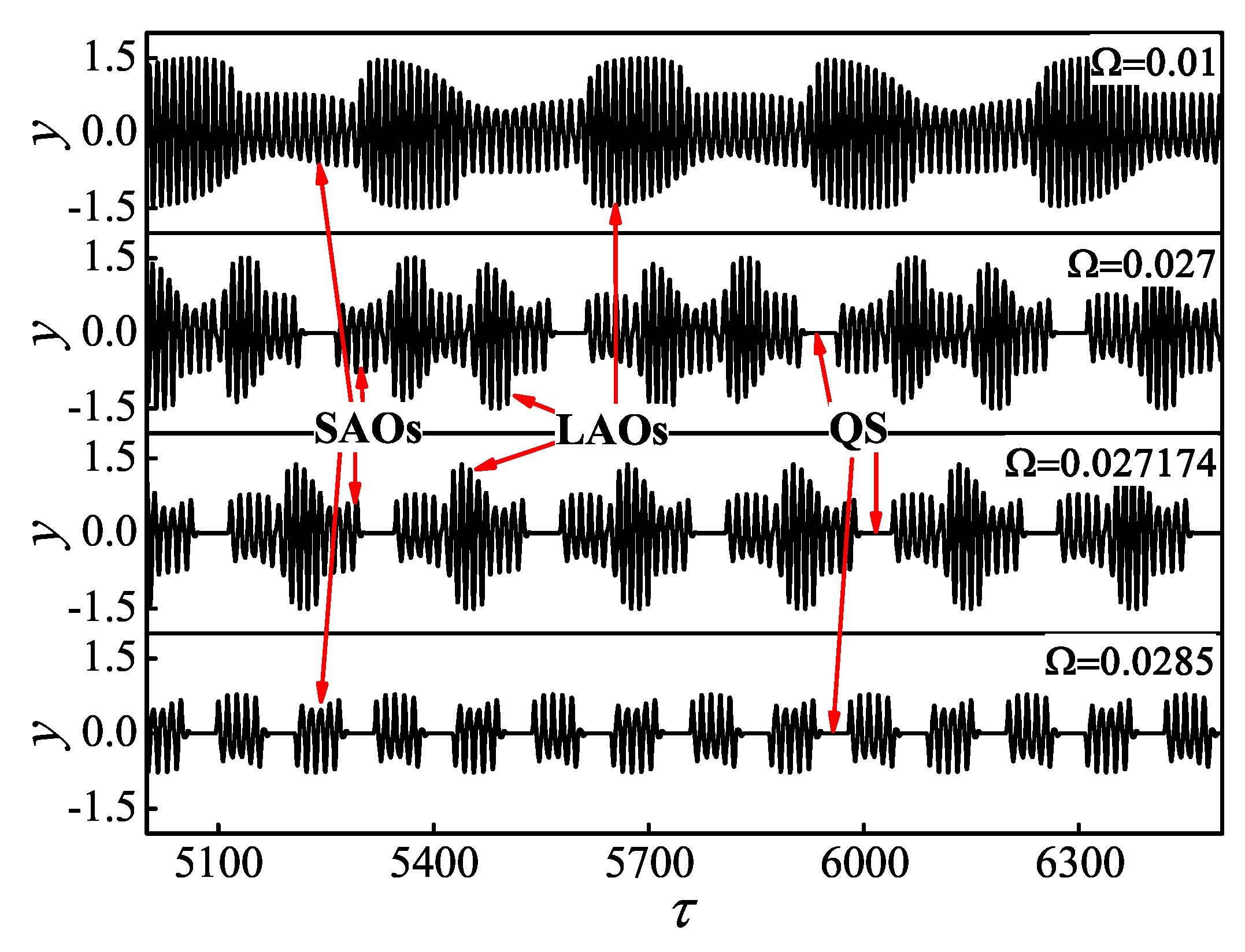
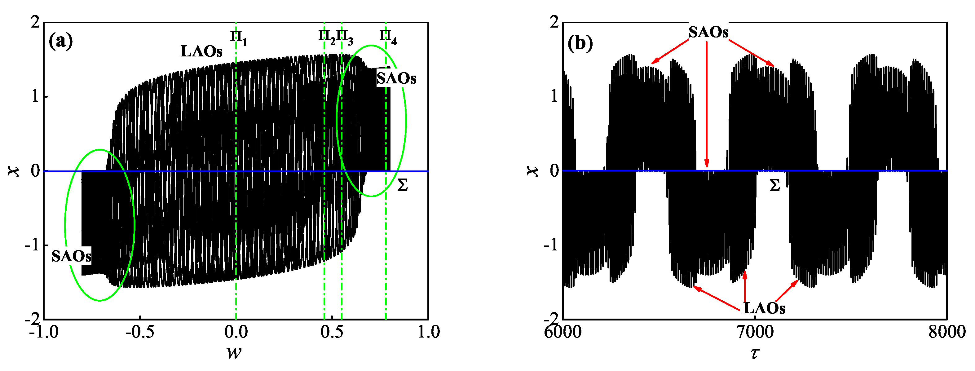
4.1. Generation Mechanism of MTSOs

Since the discontinuity boundary Σ is defined by x = 0 , we redraw the phase portrait in ( w , x ) plane and the time history of x of the MTSOs when Ω = 0.01 , respectively, given in Figure 3a,b. Then we may find that every spiking oscillation contacts the discontinuity boundary Σ (denoted as the blue horizontal line). Meanwhile, Figure 3a also reflects that the mixed tonic spiking oscillation with Ω = 0.01 may be not strictly periodic.
In order to exhibit more details about the oscillation structures, we choose Π 1 : = w = 0 , Π 2 : = w = 0.46 , Π 3 : = w = 0.55 and Π 4 : = w = 0.78 as cross sections, respectively, as shown in Figure 3a. Poincaré maps are plotted in Figure 4, where one may find that the response of the whole system (3) then is a quasi-periodic oscillation when Ω = 0.01 , since all the Poincaré maps on the four cross sections are nearly closed curves.
According to the Poincaré maps in Figure 4, it is not difficult to predict that limit cycles, i.e., the so-called spike attractors exist in the Filippov fast subsystem (4). Furthermore, the relatively large closed curves intercepted from LAOs, labeled as LAO in Figure 4a–c, indicate that the corresponding spiking attractor behaves in crossing motions on Σ . While the relatively small closed curves intercepted from SAOs, labeled as SAO in Figure 4b–d, indicate that the corresponding spiking attractor behaves in sliding motions on Σ .
The relatively small closed curves intercepted from SAOs appears in the inner of the relatively large closed curves intercepted from LAOs, seen in Figure 4b,c. It indicates that the spiking attractor behaving in crossing motions coexists with the spiking attractor behaving in sliding motions. Moreover, the relatively small closed curves intercepted from SAOs behaves in different nonsmooth structures, which means that the corresponding spiking attractor may undergo sliding bifurcation.
Considering the symmetry, as shown by the green circles in Figure 3a, two spike attractors corresponding to the two SAOs exist in (4), respectively, labeled as L C S A + ( w > 0 ) and L C S A ( w < 0 ). Taking L C S A + as the example, Figure 5 gives the corresponding geometry of sliding bifurcation, where L C S A + crosses through the visible cusp point V C on Σ S when w 0.533 to undergo a multi-sliding bifurcation, seen in Figure 5b, leading to the single sliding segment in Figure 5a turns into two sliding segments in Figure 5c.
We now discuss the generation mechanism for the quasi-periodic MTSOs when Ω = 0.01 by using the classical slow–fast decomposition method. Via analyzing the conventional bifurcations of spike attractors in Figure 6a, we can give the complete details about bifurcations of spike attractors in Table 2.
As shown by the red real arrows in Figure 6a, the relatively large amplitude spiking attractor, denoted as L C L A , will collide with the two unstable cycles L C U S ± , respectively, leading to the transitions from L C L A to L C S A ± caused by the fold bifurcations of limit cycles L P C 2 ± . Similarly, the two relatively small amplitude spike attractors L C S A ± may also collide with unstable cycles L C U S ± , respectively, leading to the transitions from L C S A ± to L C L A caused by the fold bifurcations of limit cycles L P C 1 ± .
Considering the symmetry, in order to exhibit the generation mechanism of the quasi-periodic MTSOs, we choose to superimpose one segment of trajectory with τ [ 3 π + 4 n π 2 Ω , 5 π + 4 n π 2 Ω ] ( n N * ) onto the one-parameter bifurcation diagram of spike attractors, seen in Figure 6b. During the slow variable w changes from w = 0.8 to w = 0.8 , it can be found that the evolution process of the trajectory can be explained well by using the bifurcation structures of spike attractors. For example, the multi-sliding bifurcation M S leads the SAOs behaving in single-sliding oscillations to turn into a SAO behaving in double-sliding oscillations. Meanwhile, the two fold bifurcations of limit cycles L P C 1 and L P C 2 + lead the transition from SAOs to LAOs and the transition from LAOs to SAOs, respectively.
It should be pointed out that the two multi-sliding bifurcations M S ± lead to the change of sliding modes in SAOs rather than the transitions between attractors. We will ignore these two multi-sliding bifurcations because the main focus in our work is on the transition mechanism.
Since the whole system (3) is a slow–fast dynamical system when 0 < Ω < < 1 , one may be interested in knowing whether or not the quasi-periodic MTSO response in Figure 3 should be a slow–fast dynamics behavior. The limit cycles in the fast subsystem (4) are presented in Figure 6a via giving the extreme points in the ( w , x ) plane. Without loss of generality, we can also map those limit cycles as fixed points in the ( w , x ) plane via discrete dynamics theory. As shown in Figure 6c, where F P L A , F P S A ± and F P U S ± denote the fixed points corresponding to L C L A , L C S A ± and L C U S ± , respectively, while S N 1 ± and S N 2 ± denote saddle-node bifurcations corresponding to L P C 1 ± and L P C 2 ± .
Similarly, we now represent the quasi-periodic MTSOs in Figure 3 with the maximum points of spikes, as shown by the cyan points in Figure 6c. Based on the classical slow–fast decomposition method, we can find that the quasi-periodic MTSOs is a relaxation oscillation induced by the four saddle-node bifurcations. Accordingly, we may say that the quasi-periodic MTSOs response in Figure 3 is a typical slow–fast dynamics behavior characterized by a relaxation oscillation on the torus.

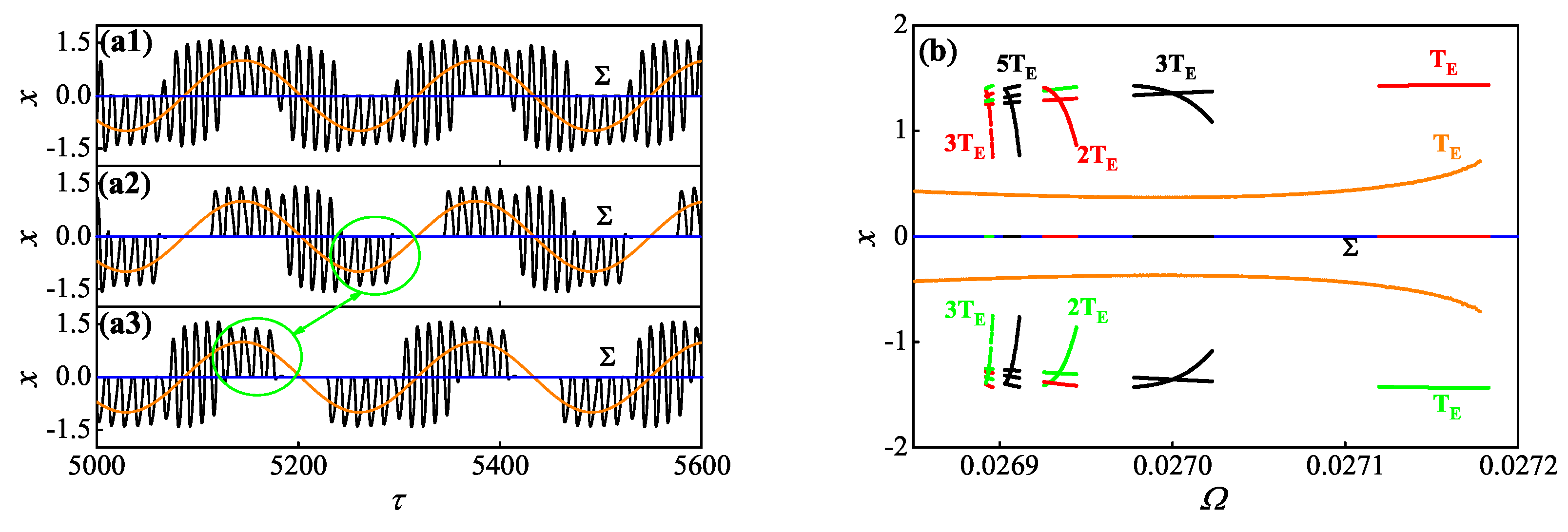
4.2. Generation Mechanism of MBOs and TBOs

Based on the above analyses for the quasi-periodic MTSOs, the response of the whole system (3) can be well predicted by attractors and the bifurcation structures in (4). Meanwhile, according to the spike attractors and bifurcations in Figure 6a, it seems that the transitions between spike attractors should be the only alternative for the whole system trajectory. However, in the MBOs when Ω = 0.027 , redrawn in Figure 7, the appearances of QSs connecting the neighboring two SAOs do not agree with the prediction based on the two fold bifurcations of limit cycles L P C 1 ± .
Figure 7 shows that the MBOs when Ω = 0.027 is a symmetrical period 3 T E response of system (3), where T E denotes the period of excitation T E = 2 π Ω . For the convenience of analysis, we divide the whole period behavior into six equal time segments in time history according to the monotonous zones of slow variable w, labeled as T i ( i = 1 , , 6 ) , respectively, seen in Figure 7b. It can be found that the QSs located on τ T 1 and τ T 4 represent the unique sticking motions which occur on discontinuity boundary Σ . Since the sticking motion is an unique nonsmooth dynamics behavior that the trajectory in Filippov systems converges to a stable PE and behaves in a certain static state, we now count PE as well as BEBs into the bifurcation diagram in Figure 6a, as shown in Figure 8a.
By employing (9) and (15) as well as the results, it is easy to check that one stable focus type pseudo-equilibrium branch P E , existing in the sliding region Σ S , will disappear at the two boundary equilibrium points X B E ± via nonsmooth fold bifurcations (respectively labeled as N F ± ). Under the separation of the four bifurcations L P C 1 ± and N F ± , seen in Figure 8a, three special rest spike bistability structures, composed by stable focus type pseudo-equilibrium points (rest attractors) and nonsmooth stable cycles (spike attractors), can be observed in the fast subsystem. One is composed of P E coexisting with the relatively large amplitude crossing cycle L C L A , while the other two are composed of P E and the small amplitude sliding cycles L C S A ± , more details are given in Table 3.
By then, the symmetrical period 3 T E MBOs in Figure 7 can be divided into two different transition routes. Taking the trajectories in decreasing intervals of the excitation as the example, as shown in Figure 8b, the segment with τ T 1 (black dash–dotted curve) and the segment with τ T 3 (black solid curve), respectively, converge to the special rest attractor P E and the crossing spike attractor L C L A . Then, the segment when τ T 1 and the segment when τ T 3 converge to the relatively small amplitude spiking attractor L C S A , respectively, caused by the bifurcation N F and the bifurcation L P C 2 .
According to the bifurcation structures presented in the fast subsystem (seen in Figure 8a), even when starting from the stable PE, the trajectories of the whole system may also transition to L C S A ± via the two nonsmooth fold bifurcations N F ± , and repeat the transition route similar with the first case with Ω = 0.01 . Clearly, the transition route in the black dash–dotted curve is non-bifurcation-induced transition. Therefore, the key to understanding the generation mechanism of MBOs in Figure 7 is to reveal the dynamics mechanism underlying the appearance of the two coexisting distinct transition routes shown in the green circle in Figure 8b, especially the fundamental reason that results in the transition from L C S A ± to P E .
One may note that the two coexisting attractors in the rest spike bistability II (III) may be very close to each other in the geometric position. For instance, see the rest spike bistability II when w = 0.445 in Figure 9a. The clockwise stable cycle L C S A + , starting from the smooth region R + ( R ), behaves in the sliding motion Γ S + ( Γ S ) when it enters into Σ S at the point P R + ( P R ), until it crosses through the sliding boundary Σ S ( Σ S + ) at the point P S ( P S + ) to enter into the opposite side of Σ . We can find that the coexisting stable P E is very close to the sliding segment Γ S . We now focus on the division of attractor basins of the two coexisting attractors in the rest spike bistability II, which is important to explain the transition route from L C S A ± to P E .
Since the stable P E is very close to the sliding segment Γ S of spike attractor L C S A + , the sliding trajectories (denoted by Φ S ( x ( τ ) , y ( τ ) , z ( τ ) ) = ( 0 , y S ( τ ) , z S ( τ ) ) ) between P E and the sliding segment Γ S will converge to one of the two coexisting attractors ultimately, According which the attractor basins of the two coexisting attractors in rest spike bistability II can be analyzed. Meanwhile considering that the sliding vector field (9) is linear, all the sliding trajectories Φ S can be derived analytically according to that P E is a stable focus, expressed by
y S ( τ ) = e τ 2 [ μ 1 ( 5 sin 35 τ 10 35 cos 35 τ 10 ) + μ 2 ( 5 cos 35 τ 10 + 35 sin 35 τ 10 ) ] 6 , z S ( τ ) = e τ 2 ( μ 1 sin 35 τ 10 + μ 2 cos 35 τ 10 ) , w ± δ α y S ( τ ) w δ α ,
where the two coefficients μ 1 , 2 can be calculated by submitting the corresponding initial conditions of a sliding trajectory Φ S into (18).
It is not difficult to verify that the two cusp points on sliding boundaries Σ S ± both are visible, computed as V C ± ( 0 , 0.445 ± 0.5 1.63 , 0.445 ± 0.5 1.63 ) via (17). Taking V C + as the initial conditions of (18), one special sliding orbit, labeled as Φ C + , can be computed with negative τ . Certainly, the sliding trajectories between P E and Φ C + will slide to the stable P E in the forward time. However, what is in doubt is whether all the sliding trajectories between Φ C + and Γ S will converge to the spike attractor L C S A + , that can be answered via the following numerical method.
One may note that all the sliding trajectories between Φ C + and Γ S inescapably cross through the visible fold points between V C + and P S + . Thus, the attractor basin structure can be easily obtained by which of the rest spike bistabilities II the trajectories from these visible fold points eventually converge to. Via numerical verification, the point P B + divides the sliding boundary Σ S + between V C + and P S + into two segments. As shown in Figure 9b,where trajectories starting from visible points between V C + and P B + converge to P E to behave in sticking motions after a minimal oscillation in R + , while trajectories starting from visible points between P B + and P S + oscillate to spike attractor L C S A + . Similarly, another special sliding orbit, denoted as Φ s e p + , can be obtained numerically by taking P B + as the initial condition of (18). It can be regarded as an attractor basin boundary of the rest spike bistability II in sliding region.
Meanwhile, the classical slow–fast decomposition method reflects a fundamental fact in the family of slow–fast dynamical systems, referring to the fact that the dynamics behaviors of the fast subsystem are modulated continuously by the slow variable. According to that, the attractor basin structures of rest spike bistability II have changed after the whole system completes one spiking oscillation. Without loss of generality, taking the trajectory oscillating along with the L C S A + in Figure 9a as the example. Assume that the whole system trajectory starts at a point in the sliding region, where the corresponding slow variable is W 1 = 0.5 sin ( 0.027 τ 1 ) , the trajectory completes a spike after one period of L C S A + (denoted as T S A + ). The slow variable has changed to be W 2 = 0.5 sin [ 0.027 ( τ 1 + T S A + ) ] , i.e., there exists a slight variation Δ w = | W 1 W 2 | . For more precision, here we name it the deviation of the slow variable (DSV for short).
Note that the excitation frequency has been assumed as 0 < Ω < < 1 , then we have Δ w 0.5 Ω T S A + , indicating that the DSV Δ w will increase along with the increase of Ω , as shown in the sketch map in Figure 10a. As we have mentioned that P E may be very close to the sliding segment Γ S of L C S A + , seen in Figure 9a, the increase in DSV caused by the increase of Ω , even though it is relatively small, can lead to unexpected influence on the attractor basins of rest spike bistability II. To illustrate this point, Figure 10b gives the attractor basin structures of rest spike bistability II with w = 0.445 , i.e., Δ w = 0 . The special sliding orbit Φ s e p + (colored in red) divides the sliding region Σ S into two different sub-regions by the aid of sliding boundary Σ S + , respectively, denoted by Σ S P and Σ S L . The sliding trajectories then converge to P E when they are located in Σ S P while the sliding trajectories converge to L C S A + (represented by the two sliding segments Γ S ± ) when they are located in Σ S L .
Interestingly, when we increase the DSV to a appropriate value, for instance, Δ w = 0.034 , another unique sliding orbit besides Φ s e p + , denoted by Φ s e p , can also be obtained numerically. Therefore, the attractor basin structures of rest spike bistability II can be redivided by using Φ s e p + as well as the two sliding boundaries Σ S ± , as shown in Figure 10c. Especially, we can find that the sliding segment Γ S then is located in Σ S P while the sliding segment Γ S + still is located in Σ S L . Sticking motions can be observed when the whole system trajectories oscillating along with L C S A + move to the sliding segment Γ S just in time. While spiking oscillations will persist when the whole system trajectories oscillating along with L C S A + move to the sliding segment Γ S + just in time.
Accordingly, one may find that a threshold Ω T exists in the whole system (3) under the parameter conditions in Table 1, which can be approximately computed as Ω T 0.025837 via tracking the critical value of Ω of the appearance of the dash-dotted transition route in Figure 8b. Therefore, we have the following results for the transitions from rest spike bistability II to rest spike bistability I. When Ω < Ω T , only the transition from L C S A + to L C L A can be observed, which is explained well by the fold bifurcation of limit cycles L P C 1 + . However, when Ω Ω T , the special transition from L C S A + to P E can also be observed besides the above. That can be explained by the disappearance of L C S A + induced by the nonnegligible DSV rather than a common bifurcation. Accordingly, we name it the transition induced by the DSV effect. Meanwhile, considering the symmetry, we have the same results about transitions from the rest spike bistability III to the rest spike bistability I.
For convenience, we can summarize the transition mechanism in a monotonous zone of slow variable w into the following two types when Ω Ω T .
  • The regular transition route, meaning that the trajectory of the whole system will transition to L C L A from L C S A ± , and then to L C S A via the fold bifurcations of limit cycles, leading to the birth of mixed tonic spiking oscillation pattern;
  • The irregular transition route, meaning that the trajectory of the whole system will transition to P E from L C S A ± via DSV effect, and then to L C S A via the nonsmooth fold bifurcations, leading to the birth of bursting oscillation pattern.
By then, the generation mechanism underlying the symmetrical period 3 T E MBOs in Figure 7 can be understood well based on the above analyses. More precisely, assuming that the trajectory starts at the maximum of w in T 1 , it, respectively, passes through the rest spike bistability II and III three times when it oscillates along with spike attractor L C S A ± , where the transition induced by DSV effect, respectively, only takes place once. It results in a symmetrically periodic transition structure composed of two irregular transitions followed by for regular transitions in a complete oscillation period. Then, the period 3 T E MBOs, consisting of two QSs characterized by sticking motions and two SPs characterized by mixed spiking oscillations, can be observed in the whole system.
Based on the analysis of the generation mechanism of the period 3 T E MBOs when Ω = 0.027 , it is not difficult to understand the responses of whole system (3) when Ω = 0.027174 and Ω = 0.0285 . We now focus on the generation mechanisms of the two responses in Figure 11.
When Ω = 0.027174 , seen in Figure 11a, we may find that the whole system (3) behaves in an asymmetrical period– 1 T E MBOs, and the trajectory, respectively, passes through the rest spike bistability II and III once when it oscillates along with spike attractor L C S A ± . The transition induced by the DSV effect only occurs when the trajectory moves to the rest spike bistability I from the rest spike bistability III, however, it does not take effect when the trajectory moves to the rest spike bistability I from the rest spike bistability II. It results in the appearance of the asymmetrical period– 1 T E MBOs consisting of one QS characterized by a sticking motion and one SP characterized by mixed spiking oscillations.
When Ω = 0.0285 , seen in Figure 11b, the whole system response is a symmetrical period– 1 T E TBOs. Similarly, with the whole system response with Ω = 0.027174 , the trajectory in this case also passes through the rest spike bistability II and III once when it oscillates along with spike attractor L C S A ± , respectively. However, we can find that the transition induced by the DSV effect may take effect at the two transition locations, leading to the trajectory transition from L C S A ± to P E . That implies the appearance of the symmetrical period– 1 T E TBOs consisting of two QSs characterized by sticking motions and two SPs characterized by spiking oscillations without LAO.

4.3. Coexistence of Whole System Responses

According to the generation mechanism of whole system responses involving transitions induced by the DSV effect, one may find that any response of the whole system is a certain combination form of regular and irregular transition routes. Moreover, such a combination may be random in theory since period–3 movement has been obtained when Ω = 0.027 , implying the appearance of an arbitrary period of whole system response, even chaos.
More interestingly, the period– 1 T E MBOs in Figure 11a is asymmetrical, i.e., there must be another asymmetrical period– 1 T E MBOs coexisting with the one in Figure 11a based on the symmetry. It indicates that the coexistence of attractors can also be observed in the whole system. We will give further discussions in this section.
Figure 12a gives the coexistence response of the whole system when Ω = 0.027174 , and the corresponding initial conditions from top to bottom are ( x ( 0 ) , y ( 0 ) , z ( 0 ) ) = ( 0 , 0.5 , 0.5 ) , ( x ( 0 ) , y ( 0 ) , z ( 0 ) ) = ( 0 , 0.5 , 0.5 ) and ( x ( 0 ) , y ( 0 ) , z ( 0 ) ) = ( 2 , 2 , 2.2 ) , respectively. Numerical results show that there also exists a symmetrical period– 1 T E MTSOs (seen in Figure 12(a1)) besides the two coexisting asymmetrical period– 1 T E MBOs (seen in Figure 12(a2,a3)), indicating that tristability then exists in the whole system (3). Noting that the asymmetrical period– 1 T E MBOs in Figure 12(a3) is symmetrical with the one in Figure 11a, the corresponding generation mechanism can be obtained according to the symmetry. Meanwhile, for the symmetrical period– 1 T E MTSOs in Figure 12(a1), the generation mechanism is attributed to the fact that only two regular transition routes appear in a complete period motion.
In order to show more details about the coexistence of responses of the whole system (3), we turn to exhibit the responses of the whole system via plotting the Poincaré map. The whole system trajectory will oscillate with L C L A when it is in the regular transition route. In contrast, the whole system trajectory may move along with P E in the irregular transition route. Accordingly, Π 1 : = w = 0 is chosen as the Poincaré cross section, which can reflect the symmetry of the whole system response and can distinguish well between the two transition routes. As shown in Figure 12b, we give the Poincaré map of the whole system when Ω ( 0.02685 , 0.027183 ) , in which the period– 1 T E MTSOs (colored in orange) can persistently exist in the whole frequency range.
Meanwhile, the period– 1 T E , period– 3 T E , period– 2 T E , period– 5 T E and period– 3 T E MBOs can discontinuously appear in turn along with the decrease of Ω . In those periodic MBOs, further numerical simulations show that the irregular transition route will appear at most once, which is absent here for brevity. Here the periodic MBOs colored in red denote the irregular transition route that only occurs nearby the rest spike bistability II. While the ones colored in green denote the irregular transition route that only occurs nearby the rest spike bistability III. Moreover, the black ones denote the irregular transition route occurs both in the rest spike bistability II and in III. Furthermore, the structures of MBOs may also alternate between asymmetry and symmetry in this progress. It leads the coexistence of responses of the whole system (3) to alternate between tristability and bistability, more details see Table 4.
Then, we can find that the whole system (3) exhibits various dynamics behaviors characterized by one period– 1 T E MTSOs coexisting with one (or two) periodic MBOs when the irregular transition route is involved. It indicates that the response only involving regular transition route still exists in the whole system when Ω Ω T . We now turn to show another interesting coexistence of the whole system responses.
When Ω = 0.0285 , tristability structure can also be observed in the whole system. As shown in Figure 13a, one symmetrical period– 1 T E TBOs, which has been presented in Figure 11b, can coexist with two asymmetrical period– 1 T E MTSOs, the corresponding initial conditions from top to bottom are ( x ( 0 ) , y ( 0 ) , z ( 0 ) ) = ( 0 , 0 , 0 ) , ( x ( 0 ) , y ( 0 ) , z ( 0 ) ) = ( 2 , 2 , 2.2 ) and ( x ( 0 ) , y ( 0 ) , z ( 0 ) ) = ( 2 , 2 , 2.2 ) , respectively. Similarly, we also give the Poincaré map when Ω ( 0.0284 , 0.02852 ) in Figure 13b, where the symmetrical period– 1 T E TBOs (colored in orange) can persistently exist in the whole frequency range. Meanwhile, both the two asymmetrical period– 1 T E MTSOs presented in Figure 13(a2,a3) perform the obvious period-doubling cascades along with the decrease of Ω , colored in light gray and gray, respectively.
Different from the former case in Figure 12b, one may find that tristability structure always exists in the whole system (3) when Ω ( 0.0284 , 0.02852 ) . Moreover, the tristability can be composed not only by a period– 1 T E TBOs coexisting with two periodic MTSOs but also by a period– 1 T E TBOs coexisting two chaotic MTSOs.

5. Conclusions and Discussions

Based on the unique rest spike bistability consisting of a limit cycle and the inner pseudo equilibrium in a Filippov slow–fast dynamical system, we have further discussed the non-bifurcation-induced transition characterized by the transition from the outside spike attractor to the inner rest attractor via various slow–fast dynamic behaviors in system (3). We found that the common feature DSV effect induced by the objective reality of timescale difference is one key factor in the transition. Furthermore, it has been proved that the DSV effect can be determined by timescale difference. In this sense, the non-bifurcation-induced transition mechanism can be regarded as the comprehensive effect of rest spike bistability and timescale difference.
Our work also reveals that there exists an essential threshold in timescale difference when a slow–fast dynamical system possesses such an interesting transition mechanism, which can be used to distinguish between transition routes across the whole system responses. As in the Filippov slow–fast dynamical system (3), the threshold Ω T under the parameter conditions in Table 1 has been given numerically. The whole system only behaves in a regular transition route that can be predicted well by bifurcation structures when Ω < Ω T . However, the irregular transition route, i.e., the non-bifurcation-induced transition route may coexist with the regular transition route when Ω > Ω T . The whole system responses then tend to be complicated and varied (shown in Figure 12b and Figure 13b). This manifests mainly in the two aspects as follows.
  • The combination form of the two coexisting transition routes may be random since the period-3 solution can be observed in the whole system responses, leading to various oscillation patterns such as multi-periodic and chaotic slow–fast dynamics behaviors.
  • Interesting and various coexistences of whole system responses can also be observed. For instance, discontinuous alternations between bistability, tristability, and persistent tristability may be performed across the whole system.
Note that the core of the classical slow–fast decomposition analysis method extensively adopted in slow–fast dynamics represents the dynamics analysis of the fast subsystem after timescale separation via the key slow variable as the bifurcation parameter. The influence of timescale difference on the whole system is ignored. On the contrary, our results show that the timescale difference must be considered in certain conditions, such as the appearance of rest spike bistability in this paper. Moreover, our numerical results indicate that the timescale difference is highly sensitive to the whole system in this regard, and thus warrants the attention of researchers in fields related to slow–fast dynamics.
A similar non-bifurcation-induced transition as that used in this paper has been involved in recent works [22,31]. However, to the best of our knowledge, we are the first to investigate that such a special transition mechanism should be a comprehensive effect of rest spike bistability and timescale difference. Furthermore, our work suggests that one non-bifurcation parameter of the fast subsystems, i.e., the excitation frequency, can also induce various slow–fast dynamic behaviors in a Filippov slow–fast dynamical system. It may provide a valuable reference for the modification and design of artificial neuron models since nearly all existing artificial neuron models are discontinuous.
Additionally, this paper mainly introduces the non-bifurcation-induced transition mechanism under the comprehensive effect of rest spike bistability and timescale difference via numerical methods. An in-depth investigation into the innate character underlying this transition mechanism and to theorize the related numerical results will prove meaningful for understanding slow–fast dynamics, which is not a trivial problem and will be our primary concern in the future.

Author Contributions

Conceptualization, S.L. and Q.B.; methodology, S.L. and Q.B.; validation, M.X. and S.L.; formal analysis, S.L.; investigation, S.L. and W.L.; writing—original draft preparation, S.L. and M.X.; writing—review and editing, S.L. and Z.C.; funding acquisition, Q.B. and W.L. All authors have read and agreed to the published version of the manuscript.

Funding

This work was supported by the National Natural Science Foundation of China (Grant Nos. 11632008, 12002299 and 11872189) and by Natural Science Foundation for Colleges and Universities in Jiangsu Province (Grant Nos. 20KJB110010).

Institutional Review Board Statement

Not applicable.

Informed Consent Statement

Not applicable.

Data Availability Statement

Not applicable.

Acknowledgments

We would like to express our deep gratitude to the anonymous referees for their valuable comments.

Conflicts of Interest

The authors declare that there is no conflict of interests regarding the publication of this manuscript.

References

  1. Chen, B.; Miller, P. Attractor-state itinerancy in neural circuits with synaptic depression. J. Math. Neurosci. 2020, 10, 15. [Google Scholar] [CrossRef] [PubMed]
  2. Curtu, R. Singular Hopf bifurcations and mixed-mode oscillations in a two-cell inhibitory neural network. Phys. D 2010, 239, 504–514. [Google Scholar] [CrossRef]
  3. Budzinski, R.C.; Lopes, S.R.; Masoller, C. Symbolic analysis of bursting dynamical regimes of Rulkov neural networks. Neurocomputing 2021, 441, 44–51. [Google Scholar] [CrossRef]
  4. Tepikin, A.V.; Petersen, O.H. Mechanisms of cellular calcium oscillations in secretory cells. BBA- Cell Res. 1992, 1137, 197–207. [Google Scholar] [CrossRef] [PubMed]
  5. Liu, P.; Liu, X.; Yu, P. Mixed-mode oscillations in a three-store calcium dynamics model. Commun. Nonlinear Sci. Numer. Simul. 2017, 52, 148–164. [Google Scholar] [CrossRef]
  6. Vishnevskii, A.L.; Elokhin, V.I.; Kutsovskaya, M.L. Dynamic model of self-oscillatory evolution in carbon monoxide oxidation over Pt(110). React. Kinet. Catal. Lett. 1993, 51, 211–217. [Google Scholar] [CrossRef]
  7. Li, X.; Bi, Q. Bursting oscillation in CO oxidation with small excitation and the enveloping slow-fast analysis method. Chin. Phys. B 2012, 21, 060505. [Google Scholar] [CrossRef]
  8. MacKay, L.; Lehman, E.; Khadra, A. Deciphering the dynamics of lamellipodium in a fish keratocytes model. J. Theor. Biol. 2020, 2020, 110534. [Google Scholar] [CrossRef]
  9. Barnhart, E.L.; Allard, J.; Lou, S.S.; Theriot, J.A.; Mogilner, A. Adhesion-dependent wave generation in crawling cells. Curr. Biol. 2017, 27, 27–38. [Google Scholar] [CrossRef] [Green Version]
  10. Bertram, R.; Rubin, J.E. Multi-timescale systems and fast–Slow analysis. Math. Biosci. 2016, 287, 105–121. [Google Scholar] [CrossRef]
  11. Prohens, R.; Teruel, A.E.; Vich, C. Slow–Fast n-dimensional piecewise linear differential systems. J. Differ. Equations 2016, 260, 1865–1892. [Google Scholar] [CrossRef]
  12. Rinzel, J.; Lee, Y.S. Dissection of a model for neuronal parabolic bursting. J. Math. Biol. 1987, 25, 653–675. [Google Scholar] [CrossRef]
  13. Rinzel, J. Formal classification of bursting mechanisms in excitable systems. In Lecture Notes in Biomathematics; Teramoto, E., Yamaguti, M., Eds.; Springer: Berlin/Heidelberg, Germany, 1987; pp. 267–281. [Google Scholar]
  14. Izhikevich, E.M. Neural excitability, spiking and bursting. Int. J. Bifurcat. Chaos 2012, 10, 1171–1266. [Google Scholar] [CrossRef] [Green Version]
  15. Han, X.; Bi, Q. Generation of hysteresis cycles with two and four jumps in a shape memory oscillator. Nonlinear Dyn. 2013, 72, 407–415. [Google Scholar] [CrossRef]
  16. Wang, Z.; Duan, L.; Cao, Q. Multi-stability involved mixed bursting within the coupled pre-Btzinger complex neurons. Chin. Phys. B 2018, 27, 070502. [Google Scholar] [CrossRef]
  17. Curtu, R.; Shpiro, A.; Rubin, N.; Rinzel, J. Mechanisms for frequency control in neuronal competition models. SIAM J. Appl. Dyn. Syst. 2008, 7, 609–649. [Google Scholar] [CrossRef] [Green Version]
  18. Buckthought, A.; Kirsch, L.E.; Fesi, J.D.; Mendola, J.D. Interocular grouping in perceptual rivalry localized with fMRI. Brain Topogr. 2021, 34, 323–336. [Google Scholar] [CrossRef]
  19. Cirillo, G.I.; Sepulchre, R. The geometry of rest-spike bistability. J. Math. Neurosci. 2020, 10, 13. [Google Scholar] [CrossRef]
  20. Kingston, S.L.; Thamilmaran, K. Bursting oscillations and mixed-mode oscillations in driven Liénard system. Int. J. Bifurcat. Chaos 2017, 27, 1730025. [Google Scholar] [CrossRef]
  21. Zhao, Y.; Liu, M.; Zhao, Y.; Duan, L. Dynamics of mixed bursting in coupled pre–Btzinger complex. Acta Phys. Sin.-Ch. Ed. 2021, 70, 120501. [Google Scholar] [CrossRef]
  22. SKuznetsov, Y.A. Elements of Applied Bifurcation Theory, 2nd ed.; Springer: New York, NY, USA, 2011. [Google Scholar]
  23. Liu, X.; Vlajic, N.; Long, X.; Meng, G.; Balachandran, B. Nonlinear motions of a flexible rotor with a drill bit: Stick-slip and delay effects. Nonlinear Dyn. 2013, 72, 61–73. [Google Scholar] [CrossRef]
  24. Moharrami, M.J.; de Martins, C.A.; Shiri, H. Nonlinear integrated dynamic analysis of drill strings under stick-slip vibration. Appl. Ocean Res. 2021, 108, 102521. [Google Scholar] [CrossRef]
  25. Depouhon, A.; Detournay, E. Instability regimes and self-excited vibrations in deep drilling systems. J. Sound Vib. 2014, 333, 2019–2039. [Google Scholar] [CrossRef] [Green Version]
  26. Yang, Y.; Liao, X. Filippov Hindmarsh-Rose Neuronal Model with Threshold Policy Control. IEEE T. Neur. Net Lear. 2018, 30, 1–6. [Google Scholar] [CrossRef]
  27. Wang, X.; Lin, X.; Dang, X. Supervised learning in spiking neural networks: A review of algorithms and evaluations. Neural Netw. 2020, 125, 258–280. [Google Scholar] [CrossRef]
  28. Kunze, M. Non-Smooth Dynamical Systems, 1st ed.; Springer: Berlin/Heidelberg, Germany, 2000. [Google Scholar]
  29. Bernardo, M.D.; Budd, C.J.; Champneys, A.R.; Kowalczyk, P. Piecewise-Smooth Dynamical Systems, 1st ed.; Springer: London, UK, 2008. [Google Scholar]
  30. Shen, B.; Zhang, Z. Complex bursting oscillations induced by bistable structure in a four-dimensional Filippov-type laser system. Pramana- Phys. Chaos 2021, 95, 97. [Google Scholar] [CrossRef]
  31. Han, H.; Bi, Q. Bursting oscillations as well as the mechanism in a Filippov system with parametric and external excitations. Int. J. Bifurcat. Chaos 2020, 30, 2050168. [Google Scholar] [CrossRef]
  32. Wang, Z.; Zhang, C.; Zhang, Z.; Bi, Q. Bursting oscillations with boundary homoclinic bifurcations in a Filippov-type Chua’s circuit. Pramana- Phys. 2020, 94, 95. [Google Scholar] [CrossRef]
  33. Qu, R.; Li, S. Attractor and vector structure analyses of bursting oscillation with sliding bifurcation in Filippov systems. Shock Vib. 2019, 2019, 1–10. [Google Scholar] [CrossRef] [Green Version]
  34. Li, S.; Han, H.; Qu, R.; Lv, W.; Bi, Q. Periodic bursting oscillations involving stick-slip motions as well as the generation mechanism in a Filippov type slow–fast dynamical system. Pramana–J. Phys. 2022; accepted. [Google Scholar]
  35. Han, X.; Bi, Q.; Kurths, J. Route to bursting via pulse-shaped explosion. Phys. Rev. E 2018, 98, 010201. [Google Scholar] [CrossRef]
  36. Wei, M.; Han, X.; Zhang, X.; Bi, Q. Bursting oscillations induced by bistable pulse-shaped explosion in a nonlinear oscillator with multiple-frequency slow excitations. Nonlinear Dyn. 2019, 99, 1301–1312. [Google Scholar] [CrossRef]
  37. Wei, M.; Jiang, W.; Ma, X.; Han, X.; Bi, Q. A new route to pulse-shaped explosion and its induced bursting dynamics. Nonlinear Dyn. 2021, 104, 4493–4503. [Google Scholar] [CrossRef]
  38. Hastings, A.; Abbott, K.C.; Cuddington, K.; Francis, T.; Gellner, G.; Lai, Y.C.; Morozov, A.; Petrovskii, S.; Scranton, K.; Zeeman, M.L. Transient phenomena in ecology. Science 2018, 361, 990. [Google Scholar] [CrossRef] [PubMed] [Green Version]
  39. Han, H.; Li, S.; Bi, Q. Non-smooth dynamics behaviors as well as the generation mechanisms in a modified Filippov type Chua’s circuit with a low-frequency external excitation. Mathematics 2022, 10, 3613. [Google Scholar] [CrossRef]
  40. Ginoux, J.M.; Llibre, J. Canards existence in memristor’s circuits. Qual. Theor. Dyn. Syst. 2016, 15, 383–431. [Google Scholar] [CrossRef] [Green Version]
  41. Marszalek, W.; Trzaska, Z. mixed-mode oscillations in a modified Chua’s circuit. Circ. Syst. Signal Pr. 2010, 29, 1075–1087. [Google Scholar] [CrossRef]
  42. Zhang, Z.; Chen, Z.; Bi, Q. Modified slow–Fast analysis method for slow–Fast dynamical systems with two scales in frequency domain. Theor. Appl. Mech. Lett. 2019, 9, 358–362. [Google Scholar] [CrossRef]
  43. Bernardo, M.D.; Kowalczyk, A.P.; Nordmarkb, A. Bifurcations of dynamical systems with sliding: Derivation of normal–form mappings. Physica D 2002, 170, 175–205. [Google Scholar] [CrossRef] [Green Version]
  44. Zhang, C.; Tang, Q. Complex periodic mixed-mode Oscillation patterns in a Filippov system. Mathematics 2022, 10, 673. [Google Scholar] [CrossRef]
Figure 1. A sketch diagram of Filippov Chua’s circuit. (a) Modified Chua’s circuit with a current source i s ; (b) the design scheme of the nonlinear resistor R N in (a).
Mathematics 10 04606 g001
Figure 2. Time histories of four responses of whole system (3) corresponding to a different excitation frequency Ω .
Mathematics 10 04606 g002
Figure 3. The MTSOs when Ω = 0.01 , which is redrawn with considering nonsmooth structures. (a) Phase portrait in ( w , x ) plane; (b) time history of fast variable x.
Mathematics 10 04606 g003
Figure 4. Poincaré maps of the MTSOs with Ω = 0.01 . (a) Π 1 : = w = 0 ; (b) Π 2 : = w = 0.46 ; (c) Π 2 : = w = 0.55 ; (d) Π 2 : = w = 0.78 .
Mathematics 10 04606 g004
Figure 5. The multi-sliding bifurcation geometry of limit cycle L C S A + , where the dark-gray region denotes sliding region Σ S and the sliding segments are colored in blue. (a) w = 0.7 ; (b) w 0.533 ; (c) w = 0.45 .
Mathematics 10 04606 g005
Figure 6. Generation mechanism analysis for the MTSOs with Ω = 0.01 . (a) One-parameter conventional bifurcation diagram of spike attractors; (b) the superimposition of one-parameter bifurcation diagram of spike attractors and one segment of trajectory with τ [ 3 π + 4 n π 2 Ω , 5 π + 4 n π 2 Ω ] ( n N * ); (c) the relaxation oscillation equivalent to the MTSOs in Figure 3.
Mathematics 10 04606 g006
Figure 7. The redrawn MBOs when Ω = 0.027 . (a) Phase portrait in ( w , x ) plane; (b) the superimposition of time history of fast variable x and the time history of slow variable w.
Mathematics 10 04606 g007
Figure 8. Rest spike bistabilities as well as the special transitions. (a) Rest spike bistabilities in the fast subsystem (4) as well as their bifurcations; (b) the superimposition of (a) and two different migration modes of whole system trajectories in the same evolution direction.
Mathematics 10 04606 g008
Figure 9. Dynamical structures of rest spike bistability II as well as the local dynamics structure. (a) Rest spike bistability II when w = 0.445 ; (b) the local dynamics structure between P E and the sliding segment Γ S .
Mathematics 10 04606 g009
Figure 10. The relationship of DSV Δ w and excitation frequency Ω as well as the influence on attractor basin structures of rest spike bistability II. (a) Sketch map of the relationship of Δ w and Ω ; (b) the attractor basin structures of rest spike bistability II in Figure 9a with Δ w = 0 ; (c) the attractor basin structures of rest spike bistability II in Figure 9a with Δ w = 0.034 .
Mathematics 10 04606 g010
Figure 11. The slow–fast decomposition of responses when Ω = 0.027174 and Ω = 0.0285 . (a) Asymmetrical period– 1 T E MBOs when Ω = 0.027174 ; (b) symmetrical period– 1 T E TBOs when Ω = 0.0285 .
Mathematics 10 04606 g011
Figure 12. Coexisting responses when Ω = 0.027174 as well as the Poincaré map of whole system. (a) The three coexisting period– 1 T E responses when Ω = 0.027174 ; (b) the Poincaré map of whole system on the section Π 1 : = w = 0 with Ω ( 0.02685 , 0.027183 ) .
Mathematics 10 04606 g012
Figure 13. Coexisting responses with Ω = 0.0285 as well as the Poincaré map of whole system. (a) The three coexisting period– 1 T E responses with Ω = 0.0285 ; (b) the Poincaré map of whole system on the section Π 1 : = w = 0 with Ω ( 0.0284 , 0.02852 ) .
Mathematics 10 04606 g013
Table 1. Parameters and their values.
Dimensionless ParameterValue
α 1.63
a−0.3
b0.5
δ −0.5
A0.8
η 0.6
Table 2. Bifurcations of spike attractors as well as the abbreviations and parameter values.
BifurcationAbbreviationParameter Value
Fold bifurcation of limit cycles L P C 2 ± w ± 0.566
Multi-sliding bifurcation M S ± w ± 0.533
Fold bifurcation of limit cycles L P C 1 ± w ± 0.444
Table 3. Rest spike bistability structures in the fast subsystem.
SortAttractorParameter RangeBorder Bifurcation
I L C L A , P E w ( 0.444 , 0.444 ) L P C 1 , L P C 1 +
II L C S A + , P E w ( 0.444 , 0.533 ) L P C 1 + , N F +
III L C S A , P E w ( 0.533 , 0.444 ) L P C 1 , N F
Table 4. Coexistence of the responses of whole system (3).
Coexistence Type Ω ZoneResponse Type
tristability ( 0.0271193 , 0.027183 ) one period– 1 T E MTSOs 1 and two period– 1 T E MBOs 2
bistability ( 0.0269777 , 0.0270228 ) one period– 1 T E MTSOs 1 and one period– 3 T E MBOs 1
tristability ( 0.0269256 , 0.0269444 ) one period– 1 T E MTSOs 1 and two period– 2 T E MBOs 2
bistability ( 0.0269029 , 0.0269114 ) one period– 1 T E MTSOs 1 and one period– 5 T E MBOs 1
tristability ( 0.0268919 , 0.0268956 ) one period– 1 T E MTSOs 1 and two period– 3 T E MBOs 2
1 Symmetrical response(s). 2 Asymmetrical response(s).
Publisher’s Note: MDPI stays neutral with regard to jurisdictional claims in published maps and institutional affiliations.

