A Comparison of Several AI Techniques for Authorship Attribution on Romanian Texts

Abstract

Determining the author of a text is a difficult task. Here, we compare multiple Artificial Intelligence techniques for classifying literary texts written by multiple authors by taking into account a limited number of speech parts (prepositions, adverbs, and conjunctions). We also introduce a new dataset composed of texts written in the Romanian language on which we have run the algorithms. The compared methods are artificial neural networks, multi-expression programming, k-nearest neighbour, support vector machines, and decision trees with C5.0. Numerical experiments show, first of all, that the problem is difficult, but some algorithms are able to generate acceptable error rates on the test set.

1. Introduction

Automated authorship attribution (AA) is defined in [1] as the task of determining authorship of an unknown text based on the textual characteristics of the text itself. Today the AA is useful in a plethora of fields: from the educational and research domain to detect plagiarism [2] to the justice domain to analyze evidence on forensic cases [3] and cyberbullying [4], to the social media [5,6] to detect compromised accounts [7].

Most approaches in the area of artificial intelligence treat the AA problem by using simple classifiers (e.g., linear SVM or decision tree) that have bag-of-words (character n-grams) as features or other conventional feature sets [8,9]. Although deep neural learning was already used for natural language processing (NLP), the adoption of such strategies for authorship identification occurred later. In recent years, pre-trained language models (such as BERT and GPT-2) have been used for finetuning and accuracy improvements [8,10,11].

The challenges in solving the AA problem can be grouped into three main groups [8]:

• The lack of large-scale datasets;
• The lack of methodological diversity;
• The ad hoc nature of authorship.

The availability of large-scale datasets has improved in recent years as large datasets have become widespread [12,13]. Other issues that relate to the datasets are the language in which the texts are written, the domain, the topic, and the writing environment. Each of these aspects has its own particularities. From the language perspective, the issue is that most available datasets consist of texts written in English. There is PAN18 [9] for English, French, Italian, Polish, and Spanish; or PAN19 [14] for English, French, Italian, and Spanish. However, there are not very many datasets for other languages and this is crucial as there are particularities that pertain to the language [15].

The methodological diversity has also improved in recent years, as it is detailed in [8]. However, the ad hoc nature of authorship is a more difficult issue, as a set of features that differentiates one author from the rest may not work for another author due to the individuality aspect of different writing styles. Even for one author, the writing style can evolve or change over a period of time, or it can differ depending on the context (e.g., the domain, the topic, or the writing environment). Thus, modeling the authorial writing style has to be carefully considered and needs to be tailored to a specific set of authors [8]. Therefore, selecting a distinguishing set of features is a challenging task.

We propose a new dataset named ROST (ROmanian Stories and other Texts) as there are few available datasets that contain texts written in Romanian [16]. The existing datasets are small, on obscure domains, or translated from other languages. Our dataset consists of 400 texts written by 10 authors. We have elements that pertain to the intended heterogeneity of the dataset such as:

• Different text types: stories, short stories, fairy tales, novels, articles, and sketches;
• Different number of texts per author: ranging from 27 to 60;
• Different sources: texts are collected from 4 different websites;
• Different text lengths: ranging from 91 to 39,195 words per text;
• Different periods: the time period in which the considered texts were written spans over 3 centuries, which introduces diachronic developments;
• Different mediums: texts were written with the intention of being read from paper medium (most of the considered authors) to online (two contemporary authors). This aspect considerably changes the writing style, as shorter sentences and shorter words are used online, and they also contain more adjectives and pronouns [17].

As our set is heterogeneous (as described above) from multiple perspectives, the authorship attribution is even more difficult. We investigate this classification problem by using five different techniques from the artificial intelligence area:

• Artificial neural networks (ANN);
• Multi-expression programming (MEP);
• K-nearest neighbor (k-NN);
• Support vector machine (SVM);
• Decision trees (DT) with C5.0.

For each of these methods, we investigate different scenarios by varying the number and the type of some features to determine the context in which they obtain the best results. The aim of our investigations is twofold. On one side, the result of this investigation is to determine which method performs best while working on the same data. On another side, we try to find out the proper number and type of features that best classify the authors on this specific dataset.

The paper is organized as follows:

• Section 2 describes the AA state of the art by using methods from artificial intelligence; details the entire prerequisite process to be considered before applying the specific AI algorithms (highlighting possible “stylometric features” to be considered); provides a table with some available datasets; presents a number of AA methods already proposed; describes the steps of the attribution process; presents an overview and a comparison of AA state-of-the-art methods.
• Section 3 details the specific particularities (e.g., in terms of size, sources, time frames, types of writing, and writing environments) of the database we are proposing and we are going to use, and the building and scaling/pruning process of the feature set.
• Section 4 introduces the five methods we are going to use in our investigation.
• Section 5 presents the results and interprets them, making a comparison between the five methods and the different sets of features used; measures the results by using metrics that allow a comparison with the results of other state-of-the-art methods.
• Section 6 concludes with final remarks on the work and provides future possible directions and investigations.

2. Related Work

The AA detection can be modeled as a classification problem. The starting premise is that each author has a stylistic and linguistic “fingerprint” in their work [18]. Therefore, in the realm of AI, this means extracting a set of characteristics, which can be identified in a large-enough writing sample [8].

2.1. Features

Stylometric features are the characteristics that define an author’s style. They can be quantified, learned [19], and classified into five groups [20]:

• Lexical (the text is viewed as a sequence of tokens grouped into sentences, with each token corresponding to a word, number, or punctuation mark):
  • Token-based (e.g., word length, sentence length, etc.);
  • Vocabulary richness (i.e., attempts to quantify the vocabulary diversity of a text);
  • Word frequencies (e.g., the traditional “bag-of-words” representation [21] in which texts become vectors of word frequencies disregarding contextual information, i.e., the word order);
  • Word n-grams (i.e., sequences of n contiguous words also known as word collocations);
  • Errors (i.e., intended to capture the idiosyncrasies of an author’s style) (requires orthographic spell checker).
• Character (the text is viewed as a sequence of characters):
  • Character types (e.g., letters, digits, etc.) (requires character dictionary);
  • Character n-grams (i.e., considers all sequences of n consecutive characters in the texts; n can have a variable or fixed length);
  • Compression methods (i.e., the use of a compression model acquired from one text to compress another text; compression models are usually based on repetitions of character sequences).
• Syntactic (text-representation which considers syntactic information):
  • Part-of-speech (POS) (requires POS tagger—a tool that assigns a tag of morpho-syntactic information to each word-token based on contextual information);
  • Chunks (i.e., phrases);
  • Sentence and phrase structure (i.e., a parse tree of each sentence is produced);
  • Rewrite rules frequencies (these rules express part of the syntactic analysis, helping to determine the syntactic class of each word as the same word can have different syntactic values based on different contexts);
  • Errors (e.g., sentence fragments, run-on sentences, mismatched use of tenses) (requires syntactic spell checker).
• Semantic (text-representation which considers semantic information):
  • Synonyms (requires thesaurus);
  • Semantic dependencies.
• Application-specific (the text is viewed from an application-specific perspective to better represent the nuances of style in a given domain):
  • Functional (requires specialized dictionaries);
  • Structural (e.g., the use of greetings and farewells in messages, types of signatures, use of indentation, and paragraph length);
  • Content-specific (e.g., content-specific keywords);
  • Language-specific.

The lexical and character features are simpler because they view the text as a sequence of word-tokens or characters, not requiring any linguistic analysis, in contrast with the syntactic and semantic characteristics, which do. The application-specific characteristics are restricted to certain text domains or languages.

A simple and successful feature selection, based on lexical characteristics, is made by using the top of the N most frequent words from a corpus containing texts of the candidate author. Determining the best value of N was the focus of numerous studies, starting from 100 [22], and reaching 1000 [23], or even all words that appear at least twice in the corpus [24]. It was observed, that depending on the value of N, different types of words (in terms of content specificity) make up the majority. Therefore, when the size of N falls within dozens, the most frequent words of a corpus are closed-class words (i.e., articles, prepositions, etc.), while when N exceeds a few hundred words, open-class words (i.e., nouns, adjectives, verbs) are the majority [20].

Even though the word n-grams approach comes as a solution to keeping the contextual information, i.e., the word order, which is lost in the word frequencies (or “bag-of-words”) approach, the classification accuracy is not always better [25,26].

The main advantage of character feature selection is that they pertain to any natural language and corpus. Furthermore, even the simplest in this category (i.e., character types) proved to be useful to quantify the writing style [27].

The character n-grams have the advantages of capturing the nuances of style and being tolerant to noise (e.g., grammatical errors or making strange use of punctuation), and the disadvantage is that they capture redundant information [20].

The syntactic feature selection requires the use of Natural Language Processing (NLP) tools to perform a syntactic analysis of texts, and they are language-dependent. Additionally, being a method that requires complex text processing, noisy datasets may be produced due to unavoidable errors made by the parser [20].

For semantic feature selection an even more detailed text analysis is required for extracting stylometric features. Thus, the measures produced may be less accurate as more noise may be introduced while processing the text. NLP tools are used here for sentence splitting, POS tagging, text chunking, and partial parsing. However, complex tasks, such as full syntactic parsing, semantic analysis, and pragmatic analysis, are hard to be achieved for an unrestricted text [20].

A comprehensive survey of the state of the art in stylometry is conducted in [28].

The most common approach used in AA is to extract features that have a high discriminatory potential [29]. There are multiple aspects that have to be considered in AA for selecting the appropriate set of features. Some of them are the language, the literary style (e.g., poetry, prose), the topic addressed by the text (e.g., sports, politics, storytelling), the length of the text (e.g., novels, tweets), the number of text samples, and the number of considered features. For instance, lexical and character features, although more simple, can considerably increase the dimensionality of the feature set [20]. Therefore, feature selection algorithms can be applied to reduce the dimensionality of such feature sets [30]. This also helps the classification algorithm to avoid overfitting on the training data.

Another prerequisite for the training phase is deciding whether the training texts are processed individually or cumulatively (per author). From this perspective, the following two approaches can be distinguished [20]:

• Instance-based approach (i.e., each training text is individually represented as a separate instance in the training process to create a reliable attribution model);
• Profile-based approach (i.e., a cumulative representation of an author’s style, also known as the author’s profile, is extracted by concatenating all available training texts of one author into one large file to flatten differences between texts).

Efstathios Stamatatos offers in [20] a comparison between the two aforementioned approaches.

2.2. Datasets

In

Table 1. Datasets used for author attribution detection; Author(s) are names of individuals who created the dataset (for a group consisting of more than two, only the name of the first person is provided in the list, followed by “et al.”); Paper is the first paper that introduced that dataset or that is recommended by its creator(s) to be used for citing the dataset; Language is the language in which the texts in the database were written; Size is the dimension of the dataset; Features stands for the types of features that can be or were used on that specific dataset (however, the information here is only indicative and should not be taken literally); No. of features, is also more an indicative value for possible feature set dimensions; Name or link provides the name by which that specific dataset is known and, when available, links are provided.

Author(s)	Paper	Language	Size	Features	No. of Features	Name or Link
Sanda-Maria Avram	this paper	Romanian	400 texts; 10 authors	conjunctions, prepositions, and adverbs	$27+85+670=782$	ROST
Shlomo Argamon and Patrick Juola	[31]	English	42 literary texts and novels; 14 authors	words, characters, n-grams	>3000	PAN11 https://pan.webis.de/data.html#pan12-attribution [32]
Patrick Juola	[33]	English	42 literary texts and novels; 14 authors	words, characters, n-grams	>3000	PAN12 https://pan.webis.de/data.html#pan12-attribution
Mike Kestemont et al.	[9]	English, French, Italian, Polish, Spanish.	2000 fanfiction texts; 20 authors	char n-gram, word n-gram, stylistic, tokens	>500	PAN18 https://pan.webis.de/data.html#pan18-authorship-attribution [34]
Mike Kestemont et al.	[35]	English, French, Italian, Spanish.	2997 cross-topic fanfiction texts; 36 authors	char n-gram, word n-gram, tokens	>300	PAN19 https://pan.webis.de/data.html#pan19-authorship-attribution [14]
Mike Kestemont et al.	[8]	English	443,000 cross-topic fanfiction texts; 278,000 authors	char n-gram, word n-gram, tokens	>300	PAN20 https://pan.webis.de/data.html#pan20-authorship-verification [36]
Daniel Pavelec et al.	[37]	Portuguese	600 articles; 20 authors	conjunctions and adverbs	$77+94=171$	−
Paulo Varela et al.	[38]	Portuguese	600 articles; 20 authors	conjunctions, adverbs, verbs and pronouns	77 + 94 + 50 + 91 = 312	−
Yanir Seroussi et al.	[39]	English	1342 legal documents; 3 authors	unigrams, n-grams	>2000	Judgment
Yanir Seroussi et al.	[40]	English	79 550 movie reviews; 62 authors	unigrams, n-grams	>200	IMDb62
Yanir Seroussi et al.	[41]	English	204 809 posts, 66 816 reviews; 22 116 users	unigrams, n-grams	>1000	IMDB1M
Efstathios Stamatatos	[42]	English	5000 newswire documents; 50 authors	unigrams, n-grams	>500	CCAT50
Efstathios Stamatatos	[43]	English	444 articles, book reviews; 13 authors	words, characters, 3-grams	>10,000	Guardian10
Efstathios Stamatatos		English	1000 CCTA industry news; 10 authors	words, characters, 3-grams	>500	C10 https://pan.webis.de/data.html#c10-attribution
Efstathios Stamatatos		English	5000 CCTA industry news; 50 authors	words, characters, n-grams	>500	C50 https://pan.webis.de/data.html#c50-attribution
Jonathan Schler et al.	[44]	English	over 600,000 posts; 19,000 bloggers	tokens, n-grams	>200	Blogs50 https://www.kaggle.com/datasets/rtatman/blog-authorship-corpus
Jade Goldstein et al.	[45]	English	756 documents; 21 authors	tokens, n-grams	>600	CMCC
Project Gutenberg		English	29,000 books; 4500 authors	tokens, n-grams	>60,000	Gutenberg https://www.gutenberg.org/

, we present a list of datasets used in AA investigations.

There is a large variation between the datasets. In terms of language, there are usually datasets with texts that are written in one language, and there are a few that have texts written in multiple languages. However, most of the available datasets contain texts written in English.

The Size column is generally the number of texts and authors that have been used in AA investigations. For example, PAN11 and PAN12 have thousands of texts and hundreds of authors. However, in the referenced paper, only a few were used. The datasets vary in the number of texts from hundreds to hundreds of thousands, and in terms of the number of authors, from tens to tens of thousands.

2.3. Strategies

According to [46], the entire process of text classification occurs in 6 stages:

• Data acquisition (from one or multiple sources);
• Data analysis and labeling;
• Feature construction and weighting;
• Feature selection and projection;
• Training of a classification model;
• Solution evaluation.

The classification process initiates with data acquisition, which is used to create the dataset. There are two strategies for the analysis and labeling of the dataset [46]: labeling groups of texts (also called multi-instance learning) [47], or assigning a label or labels to each text part (by using supervised methods) [48]. To yield the appropriate data representation required by the selected learning method, first, the features are selected and weighted [46] according to the obtained labeled dataset. Then, the number of features is reduced by selecting only the most important features and projected onto a lower dimensionality. There are two different representations of textual data: vector space representation [49] where the document is represented as a vector of feature weights, and graph representation [50] where the document is modeled as a graph (e.g., nodes represent words, whereas edges represent the relationships between the words). In the next stage, different learning approaches are used to train a classification model. Training algorithms can be grouped into different approaches [46]: supervised [48] (i.e., any machine learning process), semi-supervised [51] (also known as self-training, co-training, learning from the labeled and unlabeled data, or transductive learning), ensemble [52] (i.e., training multiple classifiers and considering them as a “committee” of decision-makers), active [53] (i.e., the training algorithm has some role in determining the data it will use for training), transfer [54] (i.e., the ability of a learning mechanism to improve the performance for a current task after having learned a different but related concept or skill from a previous task; also known as inductive transfer or transfer of knowledge across domains), or multi-view learning [55] (also known as data fusion or data integration from multiple feature sets, multiple feature spaces, or diversified feature spaces that may have different distributions of features).

By providing probabilities or weights, the trained classifier is then able to decide a class for each input vector. Finally, the classification process is evaluated. The performance of the classifier can be measured based on different indicators [46]: precision, recall, accuracy, F-score, specificity, area under the curve (AUC), and error rate. These all are related to the actual classification task. However, other performance-oriented indicators can also be considered, such as CPU time for training, CPU time for testing, and memory allocated to the classification model [56].

Aside from the aforementioned challenges, there are also other sets of issues that are currently being investigated. These are:

• Issues related to cross-domain, cross topic and/or cross-genre datasets;
• Issues related to the specificity of the used language;
• Issues regarding the style change of authors when the writing environment changes from offline to online;
• The balanced or imbalanced nature of datasets.

Some examples which focus on these types of issues, alongside their solutions and/or findings, are presented next.

Participants in the Identification Task at PAN-2018 [9], investigated two types of classifications. The corpus consists of fan-fiction texts written in English, French, Italian, Polish, and Spanish, and a set of questions and answers on several topics in English. First, they addressed the cross-domain AA, finding that heterogeneous ensembles of simple classifiers and compression models outperformed more sophisticated approaches based on deep learning. Also, the set size is inversely correlated with attribution accuracy, especially for cases when more than 10 authors are considered. Second, they investigated the detection of style changes, where single-author and multi-author texts were distinguished. Techniques ranging from machine learning ensembles to deep learning with a rich set of features have been used to detect style changes, achieving the accuracy of up to nearly 90% over the entire dataset and several reaching 100%.

The issue of cross-topic confusion is addressed in [57] for AA. This problem arises when the training topic differs from the test topic. In such a scenario, the types of errors caused by the topic can be distinguished from the errors caused by the detection of the writing style. The findings show that classification is least likely to be affected by topic variations when parts of speech are considered as features.

The analysis conducted in [58] aimed to determine which approach, such as topic or style, is better for AA. The findings showed that online news, which have a wide variety of topics, are better classified using content-based features, while texts with less topical variation (e.g., legal judgments and movie reviews) benefit from using style-based features.

In [59] it is shown that syntax (e.g., sentence structure) helps AA on cross-genre texts, while additional lexical information (e.g., parts of speech such as nouns, verbs, adjectives, and adverbs) helps to classify cross-topic and single-domain texts. It is also shown that syntax-only models may not be efficient.

Language-specific issues (e.g., the complexity and structure of sentences) are addressed in [15] in relation to the Arabic language. Ensemble methods were used to improve the effectiveness of the AA task.

The authors of [60] propose solutions to address the many issues in AA (e.g., cross-domain, language specificity, writing environment) by introducing the concept of stacked classifiers, which are built from words, characters, parts of speech n-grams, syntactic dependencies, word embeddings, and more. This solution proposes that these stacked classifiers are dynamically included in the AA model according to the input.

Two different AA approaches called “writer-dependent” and “writer-independent” were addressed in [37]. In the first approach, they used a Support Vector Machine (SVM) to build a model for each author. The second approach combined a feature-based description with the concept of dissimilarity to determine whether a text is written by a particular author or not, thereby reducing the problem to a two-class problem. The tests were performed on texts written in Portuguese. For the first approach, 77 conjunctions and 94 adverbs were used to determine the authorship and the best accuracy results on the test set composed of 200 documents from 20 different authors were 83.2%. For the second approach, the same set of documents and conjunctions was used, obtaining the best result of 75.1% accuracy. In [38], along with conjunctions and adverbs, 50 verbs and 91 pronouns were added to improve the results obtained previously, achieving a 4% improvement in both “writer-dependent” and “writer-independent” approaches.

The challenges of variations in authors’ style when the writing environment changes from traditional to online are addressed in [17]. These investigations consider changes in sentence length, word usage, readability, and frequency use of some parts of speech. The findings show that shorter sentences and words, as well as more adjectives and pronouns, are used online.

The authors of [61] proposed a feature extraction solution for AA. They investigated trigrams, bags of words, and most frequent terms in both balanced and imbalanced samples and showed with 79.68% accuracy that an author’s writing style can be identified by using a single document.

2.4. Comparison

AA is a very important and currently intensively researched topic. However, the multitude of approaches makes it very difficult to have a unified view of the state-of-the-art results. In [10], authors highlight this challenge by noting significant differences in:

• Datasets

  -

  In terms of size: small (CCAT50, CMCC, Guardian10), medium (IMDb62, Blogs50), and large (PAN20, Gutenberg);

  -

  In terms of content: cross-topic (${\times }_t$), cross-genre (${\times }_g$), unique authors;

  -

  In terms of imbalance (imb): i.e., standard deviation of the number of documents per author;

  -

  In terms of topic confusion (as detailed in [57]).

• Performance metrics

  -

  In terms of type: accuracy, F1, c@1, recall, precision, macro-accuracy, AUC, R@8, and others;

  -

  In terms of computation: even for the same performance metrics there were different ways of computing them.

• Methods

  -

  In terms of the feature extraction method,

  *

  Feature-based: n-gram, summary statistics, co-occurrence graphs;

  *

  Embedding-based: char embedding, word embedding, transformers

  *

  Feature and embedding-based: BERT.

The work presented in [10] tries to address and “resolve” these differences, bringing everything to a common denominator, even when that meant recreating some results. To differentiate between different methods, authors of [10] grouped the results in 4 classes:

• Ngram: includes character n-grams, parts-of-speech and summary statistics as shown in [57,62,63,64];
• PPM: uses Prediction by Partial Matching (PPM) compression model to build a character-based model for each author, with works presented in [28,65];
• BERT: combines a BERT pre-trained language model with a dense layer for classification, as in [66];
• pALM: the per-Author Language Model (pALM), also using BERT as described in [67].

The results of the state of the art as presented in [10] are shown in

Table 2. State of the art macro-accuracy of authorship attribution models. Information collected from [10] (Tables 1 and 3). Name is the name of the dataset; No. docs represents the number of documents in that dataset; No. auth represents the number of authors; Content indicates whether the documents are cross-topic (${\times }_t$) or cross-genre (${\times }_g$); W/D stands for words per document, representing the average length of documents; imb represents the imbalance of the dataset measured by the standard deviation of the number of documents per author.

Dataset						Macro-Accuracy (%) for Investigation Type
Name	No. Docs	No. Auth	Content	W/D	Imb	Ngram	PPM	BERT	pALM
CCAT50	5000	50	-	506	0	76.68	69.36	65.72	63.36
CMCC	756	21	${\times }_t$${\times }_g$	601	0	86.51	62.30	60.32	54.76
Guardian10	444	13	${\times }_t$${\times }_g$	1052	6.7	100	86.28	84.23	66.67
IMDb62	62,000	62	-	349	2.6	98.81	95.90	98.80	-
Blogs50	66,000	50	-	122	553	72.28	72.16	74.95	-
PAN20	443,000	278,000	${\times }_t$	3922	2.3	43.52	-	23.83	-
Gutenburg	29,000	4500	-	66,350	10.5	57.69	-	59.11	-

.

As can be seen in Table 2, the methods in the Ngram class generally work best. However, BERT-class methods can perform better on large training sets that are not cross-topic and/or cross-genre. The authors of [10] state that from their investigations it can be inferred that Ngram-class methods are preferred for datasets that have less than 50,000 words per author, while BERT-class methods should be preferred for datasets with over 100,000 words per author.

3. Proposed Dataset

The texts considered are Romanian stories, short stories, fairy tales, novels, articles, and sketches.

There are 400 such texts of different lengths, ranging from 91 to 39,195 words.

Table 3. Diversity of the considered dataset in terms of the length of the texts (i.e., number of words). Author is the author’s name (the last name is in bold); Average is the mean number of words per text written by the corresponding author; StdDev is the standard deviation; Average-Unique is the mean number of unique words; StdDev-Unique is the standard deviation on unique words; Average-Ratio is the mean number of the ratio of total words to unique words; StdDev-Ratio is the standard deviation of the ratio of total words to unique words.

Author	Average	StdDev	Average-Unique	StdDev-Unique	Average-Ratio	StdDev-Ratio
Ion Creangă	3679.34	3633.42	1061.90	719.38	3.01	0.94
Barbu Ştefănescu Delavrancea	4166.39	3702.33	1421.34	948.41	2.66	0.58
Mihai Eminescu	5854.52	7858.89	1656.96	1716.08	2.92	0.87
Nicolae Filimon	2734.32	2589.72	1040.09	729.81	2.42	0.50
Emil Gârleanu	843.05	721.06	411.19	234.71	1.88	0.32
Petre Ispirescu	3302.80	1531.36	1017.73	340.37	3.10	0.49
Mihai Oltean	553.75	484.00	282.56	201.18	1.79	0.31
Emilia Plugaru	2253.88	2667.38	756.70	581.88	2.54	0.64
Liviu Rebreanu	2284.12	1971.88	889.70	550.92	2.36	0.44
Ioan Slavici	7531.54	8969.77	1520.42	1041.40	3.96	1.62

presents the averages and standard deviations of the number of words, unique words, and the ratio of words to unique words for each author. There are differences up to almost 7000 words between the average word counts (e.g., between Slavici and Oltean). For unique words, the difference between averages goes up to more than 1300 unique words (e.g., between Eminescu and Oltean). Even the ratio of total words to unique words is a significant difference between the authors (e.g., between Slavici and Oltean).

Eminescu and Slavici, the two authors with the largest averages also have large standard deviations for the number of words and the number of unique words. This means that their texts range from very short to very long. Gârleanu and Oltean have the shortest texts, as their average number of words and unique words and the corresponding standard deviations are the smallest.

There is also a correlation between the three groups of values (pertaining to the words, unique words, and the ratio between the two) that is to be expected as a larger or smaller number of words would contain a similar proportion of unique words or the ratio of the two, while the standard deviations of the ratio of total words to unique words tend to be more similar. However, Slavici has a very high ratio, which means that there are texts in which he repeats the same words more often, and in other texts, he does not. There is also a difference between Slavici and Eminescu here because even if they have similar word count average and unique word count average, their ratio differs. Eminescu has a similar representation in terms of ratio and standard deviation with his lifelong friend Creangă, which can mean that both may have similar tendencies in reusing words.

Table 4. Diversity of the considered dataset in terms of the number of occurrences of the considered features in the texts. Author is the author’s name (the last name is in bold); Average-P is the average number of the occurrence of the considered prepositions in the texts corresponding to each author; StdDev-P is the standard deviation for the occurrence of the prepositions; Average-PA is the average number of the occurrence of the considered prepositions and adverbs; StdDev-PA is the standard deviation of the number of the occurrence of the considered prepositions and adverbs; Average-PAC is the average number of the occurrence of the considered prepositions, adverbs, and conjunctions; StdDev-PAC is the standard deviation of the number of the occurrence of the considered prepositions, adverbs, and conjunctions.

Author	Average-P	StdDev-P	Average-PA	StdDev-PA	Average-PAC	StdDev-PAC
Ion Creangă	19.90	4.94	79.21	30.11	88.34	31.86
Barbu Ştefănescu Delavrancea	19.14	3.67	73.43	27.79	81.82	29.81
Mihai Eminescu	21.85	7.18	80.04	34.11	90.04	36.22
Nicolae Filimon	18.26	3.52	61.94	18.12	70.50	19.25
Emil Gârleanu	14.65	3.01	48.12	16.11	53.21	17.19
Petre Ispirescu	19.93	3.14	79.60	17.32	89.63	18.52
Mihai Oltean	11.88	3.82	33.16	17.51	37.69	18.96
Emilia Plugaru	16.13	3.61	69.83	22.62	77.48	23.58
Liviu Rebreanu	17.25	4.07	73.88	25.65	82.62	27.37
Ioan Slavici	21.29	4.72	96.08	29.48	105.87	31.09

shows the averages of the number of features that are contained in the texts corresponding to each author. The pattern depicted here is similar to that in Table 3, which is to be expected. However, standard deviations tend to be similar for all authors. These standard deviations are considerable in size, being on average as follows:

• 4.16 on the set of 56 features (i.e., the list of prepositions),
• 23.88 on the set of 415 features (i.e., the list of prepositions and adverbs),
• 25.38 on the set of 432 features (i.e., the list of prepositions, adverbs, and conjunctions).

This means that the frequency of feature occurrence differs even in the texts written by the same author.

The considered texts are collected from 4 websites and are written by 10 different authors, as shown in

Table 5. List of authors (the author’s last name is in bold), the number of texts considered for each author (total number is in bold), and their source (i.e., the website from which they were collected).

Author	No. of Texts	https://www.povesti.org	https://povesti-ro.weebly.com/	https://ro.wikisource.org/wiki/	https://www.povesti-pentru-copii.com/
Ion Creangă	28			4	24
Barbu Ştefănescu Delavrancea	44		2	28	14
Mihai Eminescu	27			21	6
Nicolae Filimon	34			31	3
Emil Gârleanu	43		34	9
Petre Ispirescu	40		2	1	37
Mihai Oltean	32	32
Emilia Plugaru	40				40
Liviu Rebreanu	60			60
Ioan Slavici	52		3	39	10
TOTAL	400	32	41	193	134

. The diversity of sources is relevant from a twofold perspective. First, especially for old texts, it is difficult to find or determine which is the original version. Second, there may be differences between versions of the same text either because some words are no longer used or have changed their meaning, or because fragments of the text may be added or subtracted. For some authors, texts are sourced from multiple websites.

The diversity of the texts is intentional because we wanted to emulate a more likely scenario where all these characteristics might not be controlled. This is because, for future texts to be tested on the trained models, the text length, the source, and the type of writing cannot be controlled or imposed.

To highlight the differences between the time frames of the periods in which the authors lived and wrote the considered texts, as well as the environment from which the texts were intended to be read, we gathered the information presented in

Table 6. List of authors, time spans of the periods in which the authors lived and wrote the considered texts and the medium from which the readers read their texts. Author is the author’s name (the last name is in bold); Life is the lifetime of the author; Publication is the publication interval of the texts (note: the information presented here was not always easily accessible and some sources would contradict in terms of specific years, however, this information should be considered more as an indicative coordinate and should not be taken literally, the goal being that the literary texts be temporally framed in order to have a perspective on the period in which they were written/published); Century is a coarser temporal framing of the periods in which the texts were written; Medium is the environment from which most of the readers read the author’s texts.

#	Author	Life	Publication	Century	Medium
0	Ion Creangă	1837–1889	1874–1898	19th	paper
1	Barbu Ştefănescu Delavrancea	1858–1918	1884–1909	19th–20th	paper
2	Mihai Eminescu	1850–1889	1872–1865	19th	paper
3	Nicolae Filimon	1819–1865	1857–1863	19th	paper
4	Emil Gârleanu	1878–1914	1907–1915	20th	paper
5	Petre Ispirescu	1830–1887	1882–1883	19th	paper
6	Mihai Oltean	1976–	2010–2022	21th	paper and online
7	Emilia Plugaru	1951–	2010–2017	21th	paper and online
8	Liviu Rebreanu	1885–1944	1908–1935	20th	paper
9	Ioan Slavici	1848–1925	1872–1920	19th–20th	paper

. It can be seen that the considered texts were written in the time span of three centuries. This also brings an increased diversity between texts, since within such a large time span there have been significant developments in terms of language (e.g., diachronic developments), writing style relating to the desired reading medium (e.g., paper or online), topics (e.g., general concerns and concerns that relate to a particular time), and viewpoints (e.g., a particular worldview).

The diversity of the texts also pertains to the type of writing, i.e., stories, short stories, fairy tales, novels, articles, and sketches.

Table 7. List of authors and types of writing of the considered texts. Author is the author’s name (the last name is in bold); Article ${}^{*}$ include, in addition to articles written for various newspapers and magazines, other types of writing that did not fit into the other categories, but relate to this category, such as prose, essays, and theatrical or musical chronicles. Total number of texts per type are in bold.

#	Author	Novel	Story	Short Story	Fairy Tale	Article *	Sketch
0	Ion Creangă	5	12	11
1	Barbu Ştefănescu Delavrancea			37	7
2	Mihai Eminescu	1	1	4	7	14
3	Nicolae Filimon	6		5	3	20
4	Emil Gârleanu			43
5	Petre Ispirescu		1	1	38
6	Mihai Oltean			32
7	Emilia Plugaru		40
8	Liviu Rebreanu		46				14
9	Ioan Slavici		14	38
	TOTAL	12	113	171	55	35	14

shows the distribution of these types of writing among the texts belonging to the 10 authors. The difference in the type of writing has an impact on the length of the texts (for example, a novel is considerably longer than a short story), genre (for example, fairy tales have more allegorical worlds that can require a specific style of writing), the topic (for example, an article may describe more mundane topics, requiring a different type of discourse compared to the other types of writing).

Regarding the list of possible features, we selected as elements to identify the author of a text inflexible parts of speech (IPoS) (i.e., those that do not change their form in the context of communication): conjunctions, prepositions, interjections, and adverbs. Of these, we only considered those that were single-word and we removed the words that may represent other parts of speech, as some of them may have different functions depending on the context, and we did not use any syntactic or semantic processing of the text to carry out such an investigation.

We collected a list of 24 conjunctions that we checked on dexonline.ro (i.e., site that contains explanatory dictionaries of the Romanian language) not to be any other part of speech (not even among the inflexible ones). We also considered 3 short forms, thus arriving at a list of 27 conjunctions. The process of selecting prepositions was similar to that of selecting conjunctions, resulting in a list of 85 (including some short forms).

The lists of interjections and adverbs were taken from:

• https://ro.wiktionary.org/wiki/Categorie:Interjec%C8%9Bii_%C3%AEn_rom%C3%A2n%C4%83, accessed on 20 October 2022
• https://ro.wiktionary.org/wiki/Categorie:Adverbe_%C3%AEn_rom%C3%A2n%C4%83, accessed on 20 October 2022

To compile the lists of interjections and adverbs, we again considered only single-word ones and we eliminated words that may represent other parts of speech (e.g., proper nouns, nouns, adjectives, verbs), resulting in lists of 290 interjections and 670 adverbs.

The lists of the aforementioned IPoS also contain archaic forms in order to better identify the author. This is an important aspect that has to be taken into consideration (especially for our dataset which contains texts that were written over a time span of 3 centuries), as language is something that evolves and some words change as form and sometimes even as meaning or the way they are used.

From the lists corresponding to the considered IPoS features, we use only those that appear in the texts. Therefore, the actual lists of prepositions, adverbs, and conjunctions may be shorter. Details of the texts and the lists of inflexible parts of speech used can be found at reference [68].

4. Compared Methods

Below we present the methods we will use in our investigations.

4.1. Artificial Neural Networks

Artificial neural networks (ANN) is a machine learning method that applies the principle function approximation through learning by example (or based on provided training information) [69]. An ANN contains artificial neurons (or processing elements), organized in layers and connected by weighted arcs. The learning process takes place by adjusting the weights during the training process so that based on the input dataset the output outcome is obtained. Initially, these weights are chosen randomly.

The artificial neural structure is feedforward and has at least three layers: input, hidden (one or more), and output.

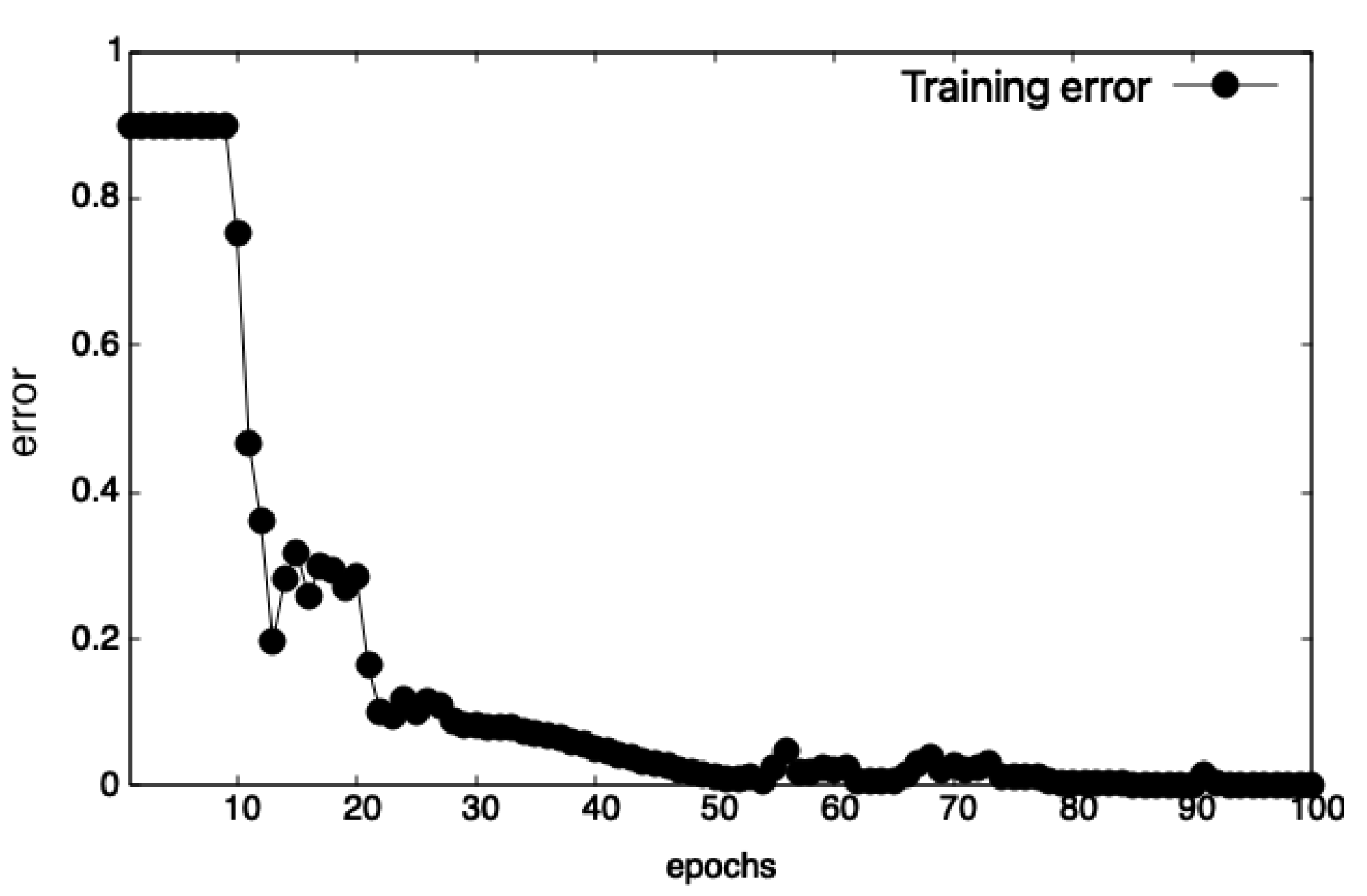
The experiments in this paper were performed using fast artificial neural network (FANN) [70] library. The error is RMSE. For the test set, the number of incorrectly classified items is also calculated.

4.2. Multi-Expression Programming

Multi-expression programming (MEP) is an evolutionary algorithm for generating computer programs. It can be applied to symbolic regression, time-series, and classification problems [71]. It is inspired by genetic programming [72] and uses three-address code [73] for the representation of programs.

MEP experiments use the MEPX software [74].

4.3. K-Nearest Neighbors

K-nearest neighbors (k-NN) [75,76,77] is a simple classification method based on the concept of instance-based learning [78]. It finds the k items, in the training set, that are closest to the test item and assigns the latter to the class that is most prevalent among these k items found.

The source code of k-NN used in this paper is written by us and is available at https://github.com/sanda-avram/ROST-source-code, (accessed on 8 November 2022) along other scripts and programs we wrote to perform the tests.

4.4. Support Vector Machine

A support vector machine (SVM) [79] is also a classification principle based on machine learning with the maximization (support) of separating distance/margin (vector). As in k-NN, SVM represents the items as points in a high-dimensional space and tries to separate them using a hyperplane. The particularity of SVM lies in the way in which such a hyperplane is selected, i.e., selecting the hyperplane that has the maximum distance to any item.

LIBSVM [80,81] is the support vector machine library that we used in our experiments. It supports classification, regression, and distribution estimation.

4.5. Decision Trees with C5.0

Classification can be completed by representing the acquired knowledge as decision trees [82]. A decision tree is a directed graph in which all nodes (except the root) have exactly one incoming edge. The root node has no incoming edge. All nodes that have outgoing edges are called internal (or test) nodes. All other nodes are called leaves (or decision) nodes. Such trees are built starting from the root by top–down inductive inference based on the values of the items in the training set. So, within each internal node, the instance space is divided into two or more sub-spaces based on the input attribute values. An internal node may consider a single attribute. Each leaf is assigned to a class. Instances are classified by running them through the tree starting from the root to the leaves.

See5 and C5.0 [83] are data mining tools that produce classifiers expressed as either decision trees or rulesets, which we have used in our experiments.

5. Numerical Experiments

To prepare the dataset for the actual building of the classification model, the texts in the dataset were shuffled and divided into training (50%), validation (25%), and test (25%) sets, as detailed in

Table 8. List of authors (the author’s last name is in bold); the number of texts and their distribution on the training, validation, and test sets. The total number of texts per author, per set, and grand total are in bold.

#	Author	No. of Texts	TrainSet Size	ValidationSet Size	TestSet Size
0	Ion Creangă	28	14	7	7
1	Barbu Ştefănescu Delavrancea	44	22	11	11
2	Mihai Eminescu	27	15	6	6
3	Nicolae Filimon	34	18	8	8
4	Emil Gârleanu	43	23	10	10
5	Petre Ispirescu	40	20	10	10
6	Mihai Oltean	32	16	8	8
7	Emilia Plugaru	40	20	10	10
8	Liviu Rebreanu	60	30	15	15
9	Ioan Slavici	52	26	13	13
	TOTAL	400	204	98	98

. In cases where we only needed training and test sets, we concatenated the validation set to the training set. We reiterated the process (i.e., shuffle and split 50%–25%–25%) three times and, thus, obtained three different training–validation–test shuffles from the considered dataset.

Before building a numerical representation of the dataset as vectors of the frequency of occurrence of the considered features, we made a preliminary analysis to determine which of the inflexible parts of speech are more prevalent in our texts. Therefore, we counted the number of occurrences of each of them based on the lists described in Section 3. The findings are detailed in

Table 9. The occurrence of inflexible parts of speech considered. IPoS stands for Inflexible part of speech; No. of occurrence is the total number of occurrences of the considered IPoS in all texts; % from total words represents the percentage corresponding to the No. of occurrence in terms of the total number of words in all texts (i.e., 1,342,133); No. of files represents the number of texts in which at least one word from the corresponding IPoS list appears; Avg. per file represents the No. of occurrence divided by the total number of texts/files (i.e., 400); and No. of IPoS represents the list length (i.e., the number of words) for each corresponding IPoS.

IPoS	No. of Occurrence	% from Total Words	No. of Files	Avg. per File	No. of IPoS
conjunctions	119,568	8.90	400	298.92	27
prepositions	176,733	13.16	400	441.83	85
interjections	6614	0.49	356	16.53	290
adverbs	127,811	9.52	400	319.52	670

.

Based on the data presented here, we decided not to consider interjections because they do not appear in all files (i.e., 44 files do not contain any interjections), and in the other files, their occurrence is much less compared to the rest of the IPoS considered. This investigation also allowed us to decide the order in which these IPoS will be considered in our tests. Thus, the order of investigation is prepositions, adverbs, and conjunctions.

Therefore, we would first consider only prepositions, then add adverbs to this list, and finally add conjunctions as well. The process of shuffling and splitting the texts into training–validation–test sets (described at the beginning of the current section, i.e., Section 5) was reiterated once more for each feature list considered. We, therefore, obtained different dataset representations, which we will refer further as described in

Table 10. Names used in the rest of the paper refer to the different dataset representations and their shuffles. Only the first 9 entries (with the Designation written in bold) were used for the entire set of investigations.

#	Designation	Features to Represent the Dataset	Shuffle
1	ROST-P-1	prepositions	#1
2	ROST-P-2	prepositions	#2
3	ROST-P-3	prepositions	#3
4	ROST-PA-1	prepositions and adverbs	#1
5	ROST-PA-2	prepositions and adverbs	#2
6	ROST-PA-3	prepositions and adverbs	#3
7	ROST-PAC-1	prepositions, adverbs and conjunctions	#1
8	ROST-PAC-2	prepositions, adverbs and conjunctions	#2
9	ROST-PAC-3	prepositions, adverbs and conjunctions	#3
10	ROST-PC-1	prepositions and conjunctions	#1
11	ROST-PC-2	prepositions and conjunctions	#2
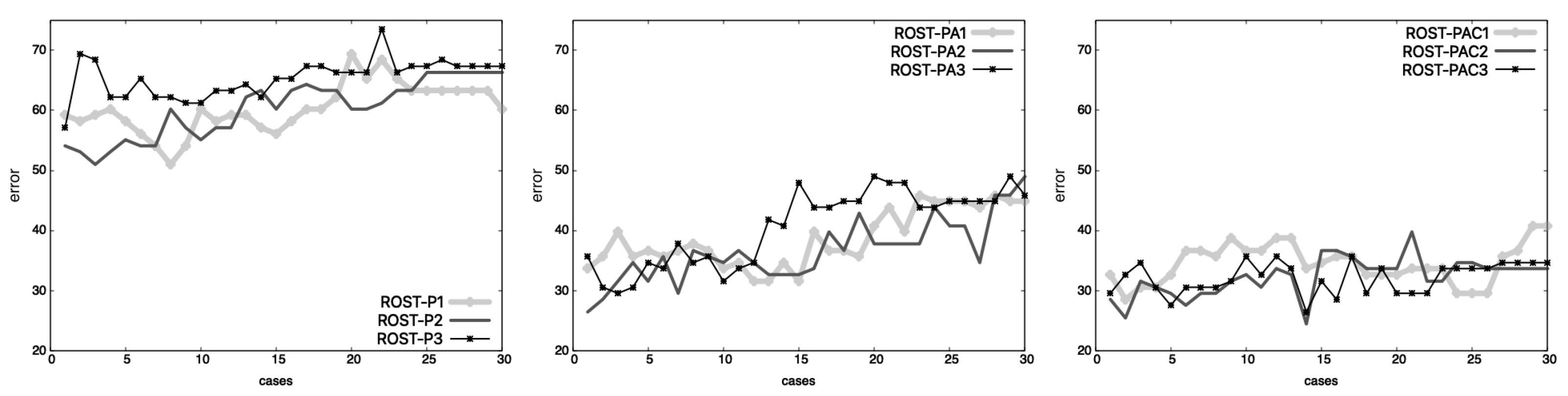
12	ROST-PC-3	prepositions and conjunctions	#3

. The last 3 entries (i.e., ROST-PC-1, ROST-PC-2, and ROST-PC-3) were used in a single experiment.

Correspondingly, we created different representations of the dataset as vectors of the frequency of occurrence of the considered feature lists. All these representations (i.e., training-validation-test sets) can be found as text files at reference [68]. These files contain feature-based numerical value representations for a different text on each line. On the last column of these files, are numbers from 0 to 9 corresponding to the author, as specified in the first columns of Table 6, Table 7 and Table 8.

5.1. Results

The parameter setting for all 5 methods are presented in Appendix A, while Appendix B contains some prerequisite tests.

Most results are presented in a tabular format. The percentages contained in the cells under the columns named Best, Avg, or Error may be highlighted using bold text or gray background. In these cases, the percentages in bold represent the best individual results (i.e., obtained by the respective method on any ROST-*-* in the dataset, out of the 9 representations mentioned above), while the gray-colored cells contain the best overall results (i.e., compared to all methods on that specific ROST-X-n representation of the dataset).

5.1.1. ANN

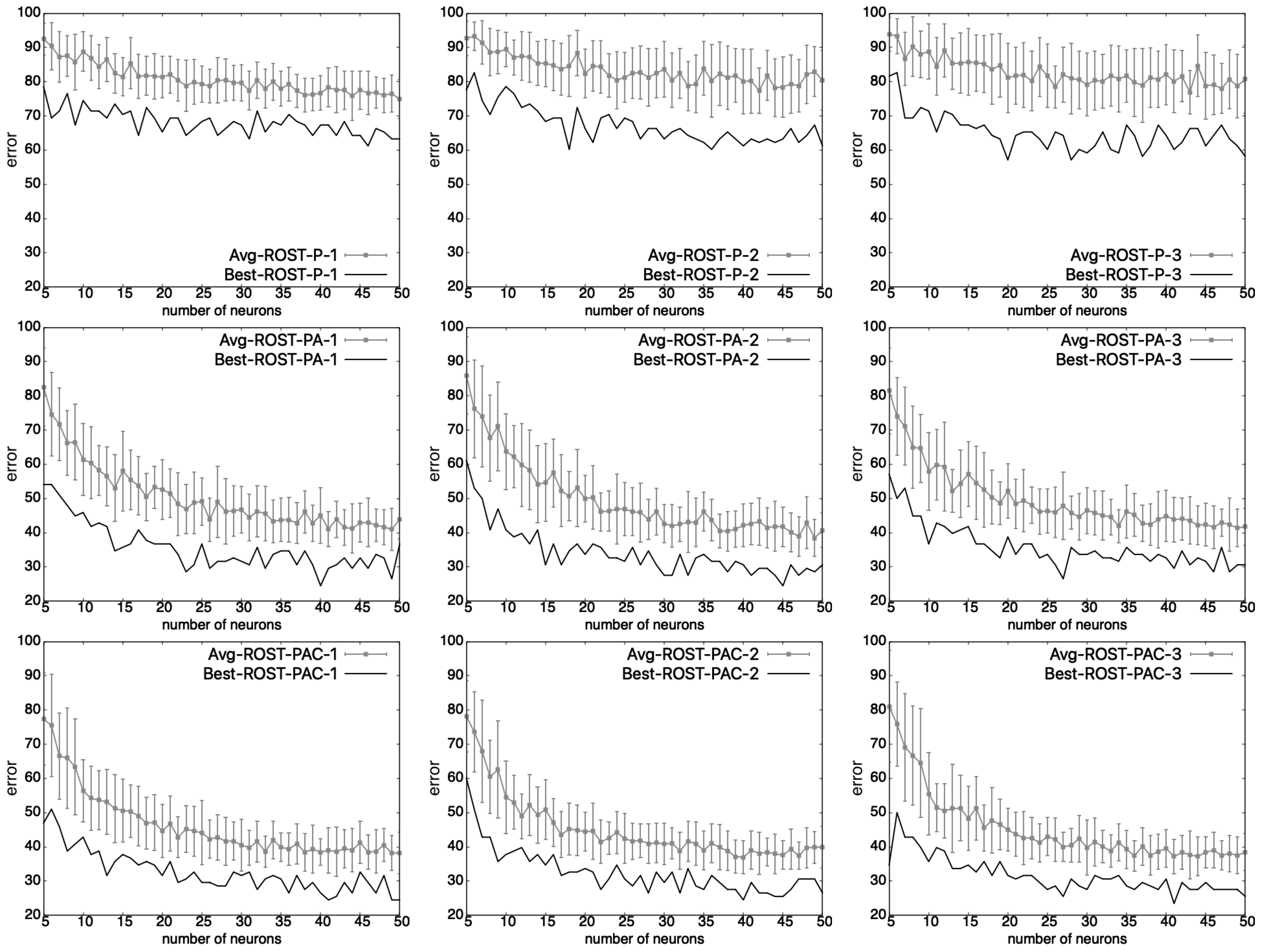
Results that showed that ANN is a good candidate to solve this kind of problem and prerequisite tests that determined the best ANN configuration (i.e., number of neurons on the hidden layer) for each dataset representation are detailed in Appendix B.1. The best values obtained for test errors and the number of neurons on the hidden layer for which these “bests” occurred are given in

Table 11. ANN results on the considered datasets. On each set, 30 runs are performed by ANNs with the hidden layer containing from 5 to 50 neurons. The number of incorrectly classified data is given as a percentage (the best results obtained by ANN on any ROST-*-* dataset representation are in bold). Best stands for the best solution (out of 30 runs on each of the 46 ANNs), Avg stands for Average (over 30 runs), StdDev stands for Standard Deviation, and No. of neurons stands for the number of neurons in the hidden layer of the ANN that produced the best solution. The best result obtained by ANN compared to all methods for a given ROST-X-n dataset representation is in a gray cell.

Dataset	Best	Avg	StdDev	No. of Neurons
ROST-P-1	61.22%	76.70%	6.30	46
ROST-P-2	60.20%	80.27%	10.58	36
ROST-P-3	57.14%	80.95%	10.30	28
ROST-PA-1	24.48%	45.03%	8.15	40
ROST-PA-2	24.48%	41.73%	5.78	45
ROST-PA-3	26.53%	47.82%	9.82	27
ROST-PAC-1	24.48%	38.16%	5.11	49
ROST-PAC-2	24.48%	36.93%	4.80	40
ROST-PAC-3	23.46%	37.21%	4.96	41

. These results show that the best test error rates were mainly generated by ANNs that have a number of neurons between 27 and 49. The best test error rate obtained with this method was $23.46\%$ for ROST-PAC-3, while the best average was $36.93\%$ for ROST-PAC-2.

5.1.2. MEP

Results that showed that MEP can handle this type of problem are described in Appendix B.2.

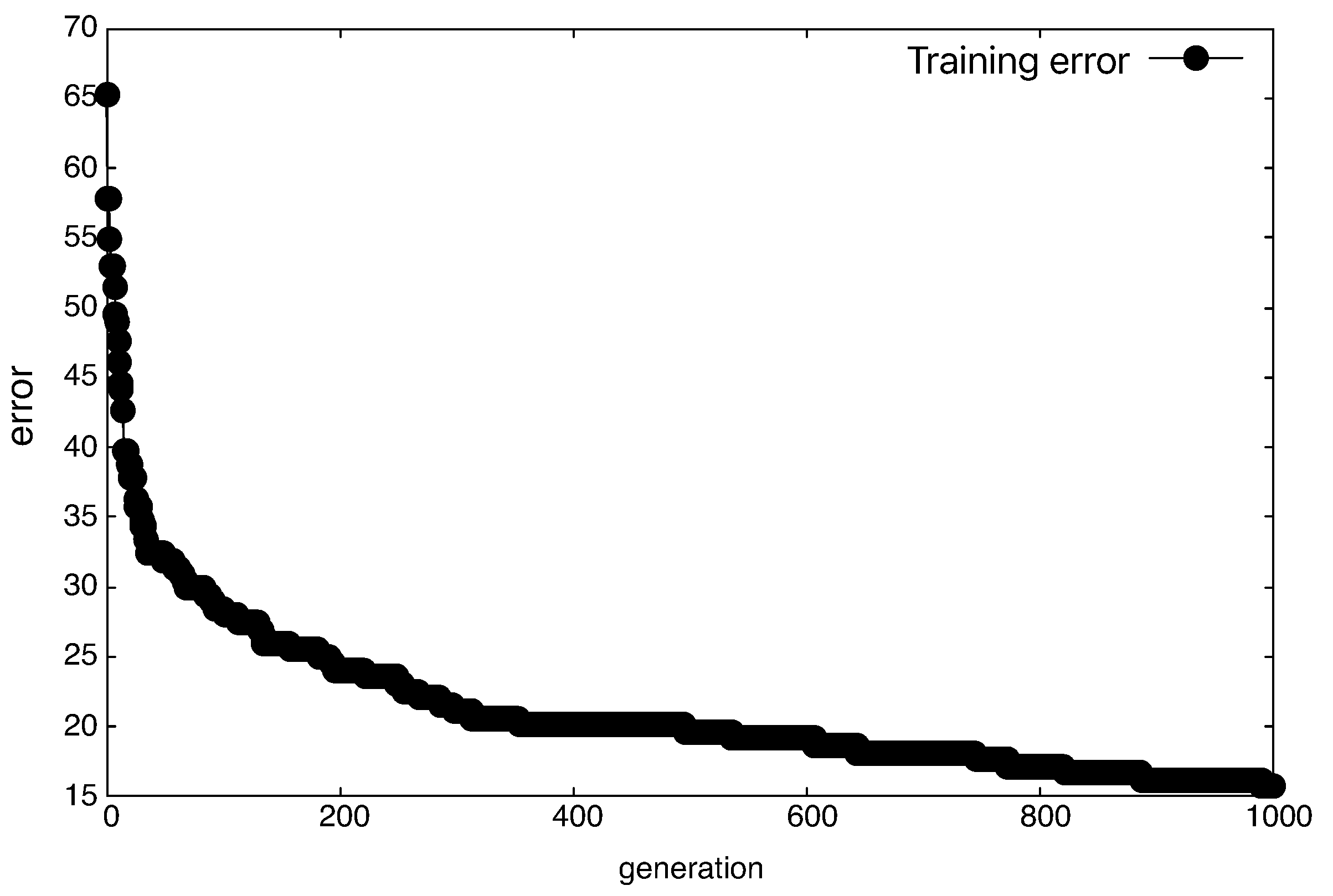
We are interested in the generalization ability of the method. For this purpose, we performed full (30) runs on all datasets. The results, on the test sets, are given in

Table 12. MEP results on the considered datasets. A total of 30 runs are performed. The number of incorrectly classified data is given as a percentage (the best results obtained by MEP on any ROST-*-* dataset representation are in bold). Best stands for the best solution (out of 30 runs), Avg stands for Average (over 30 runs) and StdDev stands for Standard Deviation. The best result obtained by MEP compared to all methods for a given ROST-X-n dataset representation is in a gray cell.

Dataset	Best	Avg	StdDev
ROST-P-1	54.08%	61.32%	4.11
ROST-P-2	52.04%	62.51%	4.46
ROST-P-3	48.97%	58.84%	4.16
ROST-PA-1	29.59%	36.49%	4.52
ROST-PA-2	20.40%	27.95%	3.87
ROST-PA-3	29.59%	39.93%	4.53
ROST-PAC-1	27.55%	33.84%	2.86
ROST-PAC-2	26.53%	34.89%	4.58
ROST-PAC-3	23.46%	34.38%	4.54

.

With this method, we obtained an overall “best” on all ROST-*-*, which is $20.40\%$, and also an overall “average” best with a value of $27.95\%$, both for ROST-PA-2.

One big problem is overfitting. The error on the training set is low (they are not given here, but sometimes are below 10%). However, on the validation and test sets the errors are much higher (2 or 3 times higher). This means that the model suffers from overfitting and has poor generalization ability. This is a known problem in machine learning and is usually corrected by providing more data (for instance more texts for an author).

5.1.3. k-NN

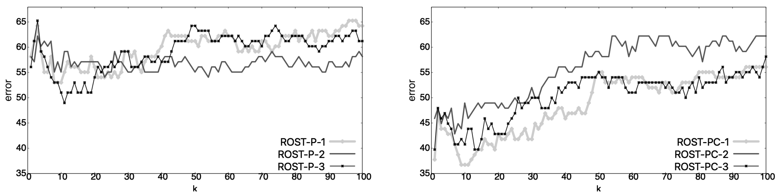
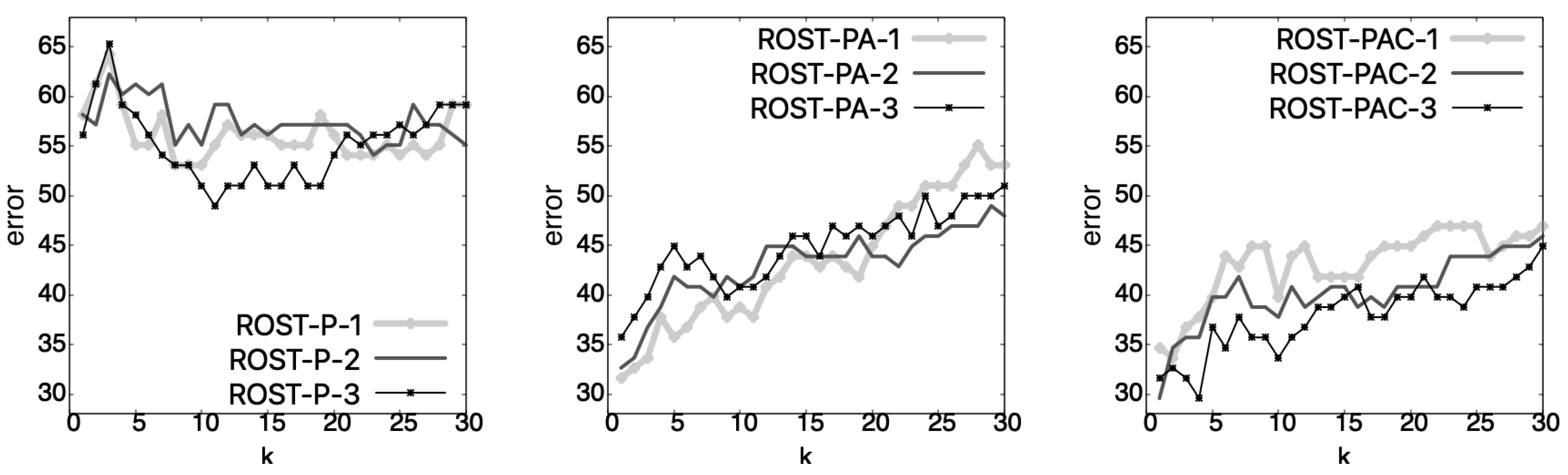
Preliminary tests and their results for determining the best value of k for each dataset representation are presented in Appendix B.3.

The best k-NN results are given in

Table 13. k-NN results on the considered datasets. In total, 30 runs are performed with k varying with the run index. The number of incorrectly classified data is given as a percentage (the best results obtained by k-MM on any ROST-*-* dataset representation are in bold). Best stands for the best solution (out of the 30 runs), k stands for the value of k for which the best solution was obtained.

Dataset	Best	k
ROST-P-1	53.06%	8
ROST-P-2	54.08%	23
ROST-P-3	48.97%	11
ROST-PA-1	31.63%	1
ROST-PA-2	32.6%	1
ROST-PA-3	35.71%	1
ROST-PAC-1	33.67%	2
ROST-PAC-2	29.59%	1
ROST-PAC-3	29.59%	4

with the corresponding value of k for which these “bests” were obtained. It can be seen that for all ROST-P-*, the values of k were higher (i.e., $k\ge 8$) than those for ROST-PA-* or ROST-PAC-* (i.e., $k\le 4$). The best value obtained by this method was $29.59\%$ for ROST-PAC-2 and ROST-PAC-3.

5.1.4. SVM

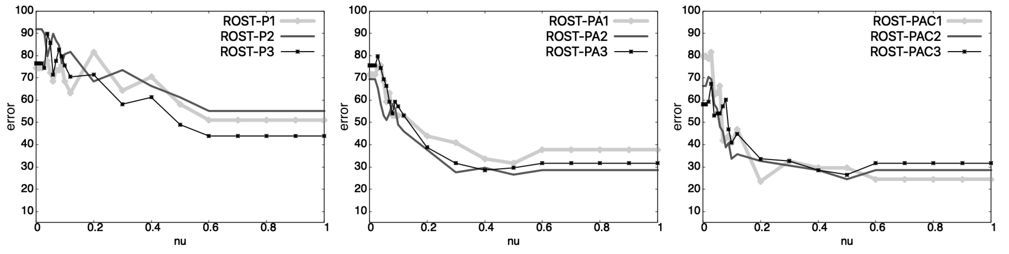
Prerequisite tests to determine the best kernel type and a good interval of values for the parameter $nu$ are described in Appendix B.4, along with their results.

We ran tests for each kernel type and with nu varying from 0.1 to 1, as we saw in Figure A6 that for values less than 0.1, SVM is unlikely to produce the best results. The best results obtained are shown in

Table 14. SVM results on the considered datasets. The number of incorrectly classified data is given as a percentage (the best results obtained by SVM on any ROST-*-* dataset representation are in bold). Best stands for the best test error rate (out of 30 runs with $nu$ ranging from 0.001 to 1), and nu stands for the parameter specific to the selected type of SVM (i.e., nu-SVC). Results are given for each type of kernel that was used by the SVM. The best result obtained by SVM compared to all methods for a given ROST-X-n dataset representation is in a gray cell.

	Linear Kernel		Polynomial Kernel		Radial Basis Kernel		Sigmoid Kernel
Dataset	Best	nu	Best	nu	Best	nu	Best	nu
ROST-P-1	43.87%	≥$0.6$	65.30%	0.5	59.18%	0.4	58.16%	0.4
ROST-P-2	55.10%	≥$0.6$	70.40%	0.2, 0.4	67.34%	0.4	68.37%	0.2, 0.4
ROST-P-3	43.87%	≥$0.6$	65.30%	0.5	59.18%	0.4	58.16%	0.4
ROST-PA-1	31.63%	0.5	51.02%	0.5	44.89%	0.3	45.91%	0.3
ROST-PA-2	26.53%	0.5	55.10%	≥$0.6$	44.89%	≥$0.6$	44.89%	≥$0.6$
ROST-PA-3	28.57%	0.4	54.08%	0.2, 0.3	51.02%	0.2	51.02%	0.2
ROST-PAC-1	23.46%	0.2	54.08%	0.2	50.00%	0.5	50.00%	0.5
ROST-PAC-2	24.48%	0.5	51.02%	≥$0.6$	39.79%	≥$0.6$	39.79%	≥$0.6$
ROST-PAC-3	26.53%	0.5	51.02%	0.4	41.83%	0.5	42.85%	0.5

.

As can be seen, the best values were obtained for values of parameter nu between 0.2 and 0.6 (where sometimes 0.6 is the smallest value of the set {0.6, 0.7, ⋯, 1} for which the best test error was obtained). The best value obtained by this method was $23.46\%$ for ROST-PAC-1, using the linear kernel and nu parameter value 0.2.

5.1.5. Decision Trees with C5.0

Advanced pruning options for optimizing the decision trees with C5.0 model and their results are presented in Appendix B.5. The best results were obtained by using $-m$ cases option, as detailed in

Table 15. Decision tree results on the considered datasets. The number of incorrectly classified data is given as a percentage (the best results obtained by DT with C5.0 on any ROST-*-* dataset representation are in bold). Error stands for the test error rate, Size stands for the size of the decision tree required for that specific solution and cases stands for the threshold for which is decided to have two more that two branches at a specific branching point ($cases\in \{1,2,\cdots ,30\}$). The best result obtained by DT with C5.0 compared to all methods for a given ROST-X-n dataset representation is in a gray cell.

Dataset	Error	Size	Cases
ROST-P-1	51.0%	18	8
ROST-P-2	51.0%	46	3
ROST-P-3	57.1%	99	1
ROST-PA-1	31.6%	13	12
ROST-PA-2	26.5%	57	1
ROST-PA-3	29.6%	31	3
ROST-PAC-1	28.6%	39	2
ROST-PAC-2	24.5%	12	14
ROST-PAC-3	26.5%	13	14

.

The best result obtained by this method was $24.5\%$ on ROST-PAC-2, with $-m$ 14 option, on a decision tree of size 12. When no options were used, the size of the decision trees was considerably larger for ROST-P-* (i.e., ≥57) than those for ROST-PA-* and ROST-PAC-* (i.e., ≤39).

5.2. Comparison and Discussion

The findings of our investigations allow for a twofold perspective. The first perspective refers to the evaluation of the performance of the five investigated methods, as well as to the observation of the ability of the considered feature sets to better represent the dataset for successful classification. The other perspective is to place our results in the context of other state-of-the-art investigations in the field of author attribution.

5.2.1. Comparing the Internally Investigated Methods

From all the results presented above, upon consulting the tables containing the best test error rates, and especially the gray-colored cells (which contain the best results while comparing the methods amongst themselves) we can highlight the following:

• ANN:

  -

  Four best results for: ROST-PA-1, ROST-PA-3, ROST-PAC-2 and ROST-PAC-3 (see Table 11);

  -

  Best ANN 23.46% on ROST-PAC-3; best ANN average 36.93% on ROST-PAC-2;

  -

  Worst best overall $61.22\%$ on ROST-P-1.

• MEP:

  -

  Two best results for ROST-PA-2 and ROST-PAC-3 (see Table 12);

  -

  Best overall 20.40% on ROST-PA-2; best overall average 27.95% on ROST-PA-2;

  -

  Worst best MEP $54.08\%$ on ROST-P-1.

• k-NN:

  -

  Zero best results (see Table 13);

  -

  Best k-NN 29.59% on ROST-PAC-2 and ROST-PAC-3;

  -

  Worst k-NN $54.08\%$ on ROST-P-2.

• SVM:

  -

  Four best results for: ROST-P-1, ROST-P-3, ROST-PAC-1 and ROST-PAC-2 (see Table 14);

  -

  Best SVM 23.44% on ROST-PAC-1;

  -

  Worst SVM $52.10\%$ on ROST-P-2.

• Decision trees:

  -

  Two best results for: ROST-P-2 and ROST-PAC-2 (see Table 15);

  -

  Best DT 24.5% on ROST-PAC-2;

  -

  Worst DT $57.10\%$ on ROST-P-2.

Other notes from the results are:

• Best values for each method were obtained for ROST-PA-2 or ROST-PAC-*;
• The worst of these best results were obtained for ROST-P-1 or ROST-P-2;
• ANN and MEP suffer from overfitting. The training errors are significantly smaller than the test errors. This problem can only be solved by adding more data to the training set.

An overview of the best test results obtained by all five methods is given in

Table 16. Top of methods on each shuffle of each dataset, based on the best results achieved by each method. The gray-colored box represents the overall best (i.e., for all datasets and with all methods).

Dataset	1st Place	2nd Place	3rd Place	4th Place	5th Place
ROST-P-1	SVM	DT	k-NN	MEP	ANN
	43.87%	51.0%	53.06%	54.08%	61.22%
ROST-P-2	DT	MEP	k-NN	SVM	ANN
	51.0%	52.04%	54.08%	55.10%	60.20%
ROST-P-3	SVM	k-NN,MEP		DT,ANN
	43.87%	48.97%		57.14%
ROST-PA-1	ANN	MEP	SVM,DT,k-NN
	24.48%	29.59%	31.63%
ROST-PA-2	MEP	ANN	SVM,DT		k-NN
	20.40%	24.48%	26.53%		32.6%
ROST-PA-3	ANN	SVM	MEP,DT		k-NN
	26.53%	28.57%	29.59%		35.71%
ROST-PAC-1	SVM	ANN	MEP	DT	k-NN
	23.46%	24.48%	27.55%	28.6%	33.67%
ROST-PAC-2	SVM,DT,ANN			MEP	k-NN
	24.48%			26.53%	29.59%
ROST-PAC-3	MEP,ANN		SVM,DT		k-NN
	23.46%		26.53%		29.59%

.

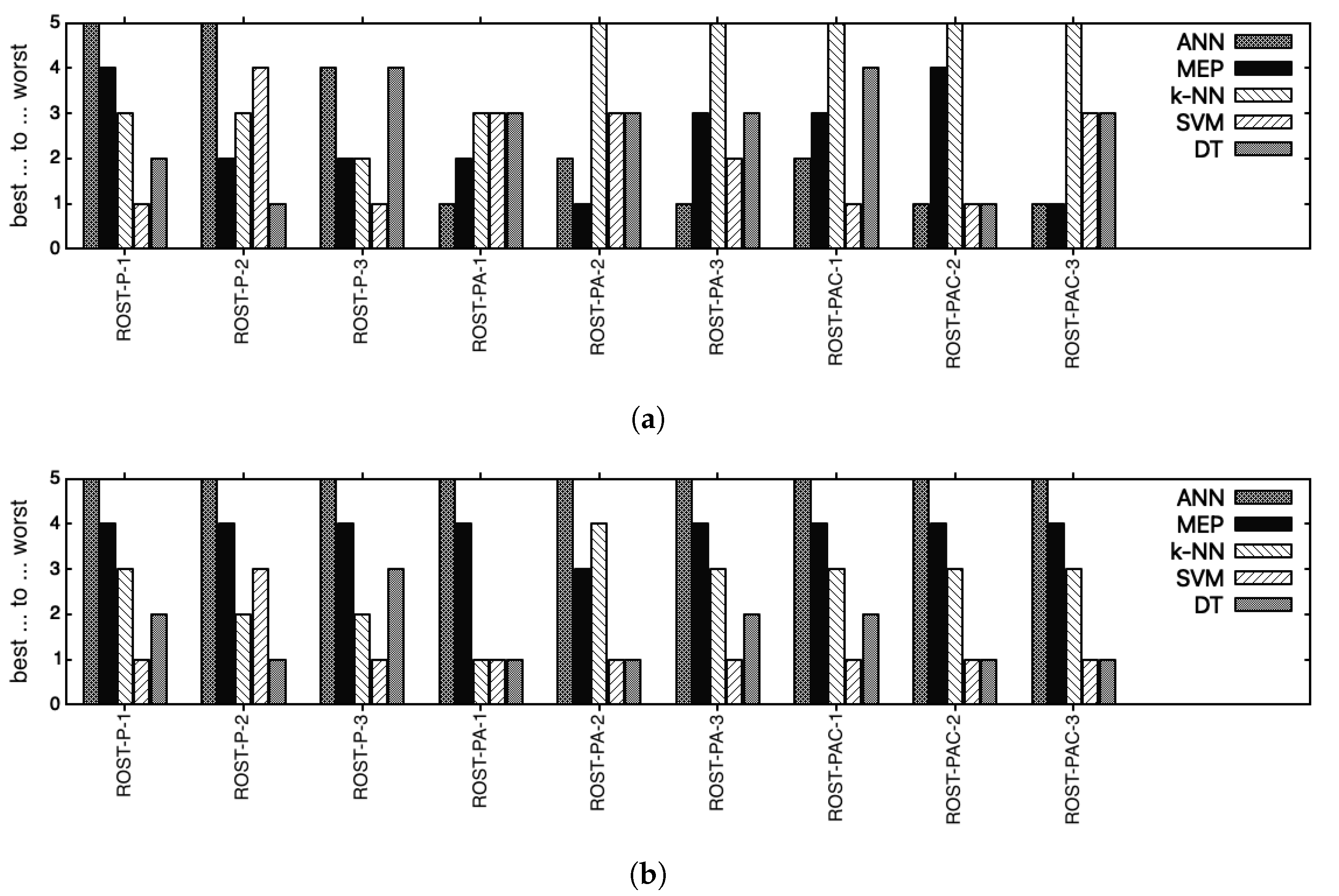
ANN ranks last for all ROST-P-* and ranks 1st and 2nd for ROST-PA-* and ROST-PAC-*. MEP is either ranked 1st or ranked 2nd on all ROST-*-* with three exceptions, i.e., for ROST-P-1 and ROST-PAC-2 (at 4th place) and for ROST-PAC-1 (at 3rd place). k-NN performs better (i.e., 3rd and 2nd places) on ROST-P-*, and ranks last for ROST-PA-* and ROST-PAC-*. SVM is ranked 1st for ROST-P-* and ROST-PAC-* with two exceptions: for ROST-P-2 (ranked 4th) and for ROST-PAC-3 (on 3rd place). For ROST-PA-* SVM is in 3rd and 2nd places. Decision trees (DT) with C5.0 is mainly on the 3rd and 4th places, with three exceptions: for ROST-P-1 (on 2nd place), for ROST-P-2 (on 1st place), and for ROST-PAC-2 (on 1st place).

An overview of the average test results obtained by all five methods is given in

Table 17. Top of methods on average results on each shuffle of each dataset. For k-NN, SVM, and DT we do not have 30 runs with the same parameters, so for these methods, the best values are presented here. The gray-colored box represents the overall best average (i.e., on all datasets and with all methods).

Dataset	1st Place	2nd Place	3rd Place	4th Place	5th Place
ROST-P-1	SVM	DT	k-NN	MEP	ANN
	43.87%	51.0%	53.06%	61.32%	76.70%
ROST-P-2	DT	k-NN	SVM	MEP	ANN
	51.0%	54.08%	55.10%	62.51%	80.27%
ROST-P-3	SVM	k-NN	DT	MEP	ANN
	43.87%	48.97%	57.14%	58.84%	80.95%
ROST-PA-1	SVM,DT,k-NN			MEP	ANN
	31.63%			36.49%	45.03%
ROST-PA-2	SVM,DT		MEP	k-NN	ANN
	26.53%		27.95%	32.6%	41.73%
ROST-PA-3	SVM	DT	k-NN	MEP	ANN
	28.57%	29.59%	35.71%	39.93%	47.82%
ROST-PAC-1	SVM	DT	k-NN	MEP	ANN
	23.46%	28.6%	33.67%	33.84%	38.16%
ROST-PAC-2	SVM,DT		k-NN	MEP	ANN
	24.48%		29.59%	34.89%	36.93%
ROST-PAC-3	SVM,DT		k-NN	MEP	ANN
	26.53%		29.59%	34.38	37.21%

. However, for ANN and MEP alone, we could generate different results with the same parameters, based on different starting seed values, with which we ran 30 different runs. For the other 3 methods, we used the best results obtained with a specific set of parameters (as in Table 16).

Comparing all 5 methods based on averages, SVM and DT take the lead as the two methods that share the 1st and 2nd places with two exceptions, i.e., for ROST-P-2 and ROST-P3 for which SVM and DT, respectively, rank 3rd. k-NN usually ranks 3rd, with four exceptions, when k-NN was ranked 2nd for ROST-P-2 and ROST-P-3, for ROST-PA-1 for which k-NN ranks 1st together with SVM and DT, and for ROST-PA-2 for which k-NN ranks 4th. MEP is generally ranked 4th with one exception, i.e., for ROST-PA-2 for which it ranks 3rd. ANN ranks last for all ROST-*-*.

For a better visual representation, we have plotted the results from Table 16 and Table 17 in Figure 1.

We performed statistical tests to determine whether the results obtained by MEP and ANN are significantly different with a 95% confidence level. The tests were two-sample, equal variance, and two-tailed T-tests. The results are shown in

Table 18. p-values obtained when comparing MEP and ANN results over 30 runs. No. of neurons used by ANN on the hidden layer represents the best-performing ANN structure on the specific ROST-*-*.

Dataset	p-Value (ANN vs. MEP Results)	No. of Neurons Used by ANN on the Hidden Layer
ROST-P-1	1.98 $\times {10}^{-15}$	46
ROST-P-2	4.23 $\times {10}^{-11}$	36
ROST-P-3	3.86 $\times {10}^{-15}$	28
ROST-PA-1	1.14 $\times {10}^{-5}$	40
ROST-PA-2	6.57 $\times {10}^{-15}$	45
ROST-PA-3	3.07 $\times {10}^{-4}$	27
ROST-PAC-1	2.47 $\times {10}^{-4}$	49
ROST-PAC-2	1.07 $\times {10}^{-1}$	40
ROST-PAC-3	2.80 $\times {10}^{-2}$	41

.

The p-values obtained show that the MEP and ANN test results are statistically significantly different for almost all ROST-*-* (i.e., $p<0.05$) with one exception, i.e., for ROST-PAC-2 for which the differences are not statistically significant (i.e., $p=0.107$).

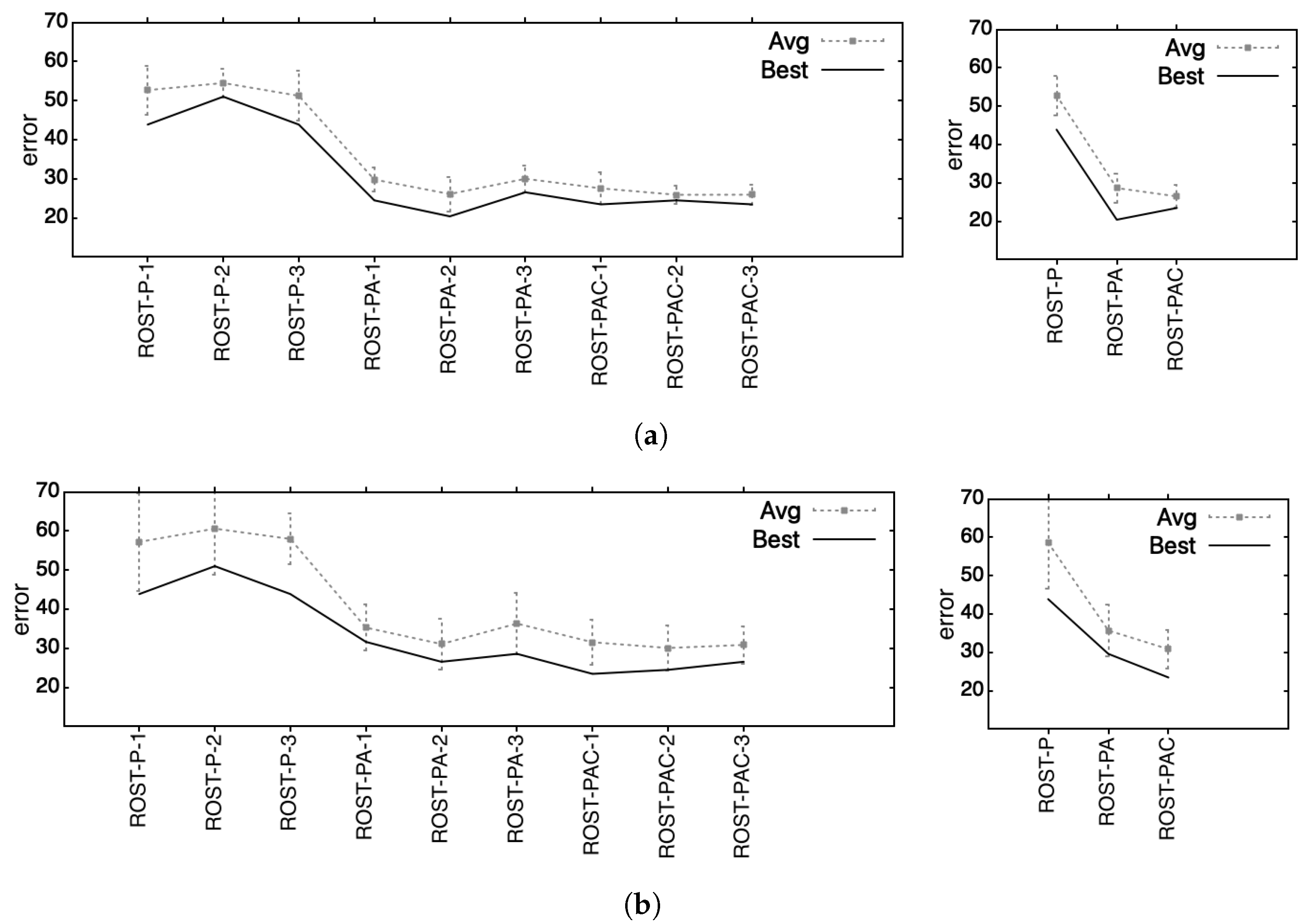
Next, we wanted to see which feature set, out of the three we used, was the best for successful author attribution. Therefore, we plotted all best and best average results obtained with all methods (as presented in Table 16 and Table 17) on all ROST-*-* and aggregated on the three datasets corresponding to the distinct feature lists, in Figure 2.

Based on the results represented in Figure 2a (i.e., which considered only the best results, as detailed in Table 16) we can conclude that we obtained the best results on ROST-PA-* (i.e., corresponding to the 415 feature set, which contains prepositions and adverbs). However, using the average results, as shown in Figure 2b and detailed in Table 17 we infer that the best performance is obtained on ROST-PAC-* (i.e., corresponding to the 432-feature set, containing prepositions, adverbs, and conjunctions).

Another aspect worth mentioning based on the graphs presented in Figure 2 is related to the standard deviation (represented as error bars) between the results obtained by all methods considered on all considered datasets. Standard deviations are the smallest in Figure 2a, especially for ROST-PA-* and even more so for ROST-PAC-*. This means that the methods perform similarly on those datasets. For ROST-P-* and in Figure 2b, the standard deviations are larger, which means that there are bigger differences between the methods.

5.2.2. Comparisons with Solutions Presented in Related Work

To better evaluate our results and to better understand the discriminating power of the best performing method (i.e., MEP on ROST-PA-2), we also calculate the macro-accuracy (or macro-average accuracy). This metric allows us to compare our results with the results obtained by other methods on other datasets, as detailed in Table 2. For this, we considered the test for which we obtained our best result with MEP, with a test error rate of 20.40%. This means that 20 out of 98 tests were misclassified.

To perform all the necessary calculations, we used the Accuracy evaluation tool available at [84], build based on the paper [85]. By inputting the vector of targets (i.e., authors/classes that were the actual authors (i.e., correct classifications) of the test texts) and the vector of outputs (i.e., authors/classes identified by the algorithm as the authors of the test texts), we were first given a Confusion value of $0.2$ and the Confusion Matrix, depicted in

Table 19. Confusion Matrix (on the right side). Column headers and row headers (i.e., numbers from 0 to 9 that are written in bold) are the codes ¹ given to our authors, as specified on the left side.

Code	Author		0	1	2	3	4	5	6	7	8	9
0	Ion Creangă	0	6	0	0	0	0	0	0	0	0	1
1	Barbu Ştefănescu Delavrancea	1	0	4	0	3	1	0	1	0	0	2
2	Mihai Eminescu	2	0	0	6	0	0	0	0	0	0	0
3	Nicolae Filimon	3	0	1	1	6	0	0	0	0	0	0
4	Emil Gârleanu	4	1	1	0	0	6	0	0	0	1	1
5	Petre Ispirescu	5	0	0	0	0	0	10	0	0	0	0
6	Mihai Oltean	6	0	0	0	0	0	0	8	0	0	0
7	Emilia Plugaru	7	0	1	0	0	1	0	0	8	0	0
8	Liviu Rebreanu	8	0	1	0	0	0	0	1	0	12	1
9	Ioan Slavici	9	0	0	0	0	0	0	0	0	1	12

¹ The authors’ codes are the same as those specified in the first columns of Table 6, Table 7 and Table 8.

.

This matrix is a representation that highlights for each class/author the true positives (i.e., the number of cases in which an author was correctly identified as the author of the text), the true negatives (i.e., the number of cases where an author was correctly identified as not being the author of the text), the false positives (i.e., the number of cases in which an author was incorrectly identified as being the author of the text), the false negatives (i.e., the number of cases where an author was incorrectly identified as not being the author of the text). For binary classification, these four categories are easy to identify. However, in a multiclass classification, the true positives are contained in the main diagonal cells corresponding to each author, but the other three categories are distributed according to the actual authorship attribution made by the algorithm.

For each class/author, various metrics are calculated based on the confusion matrix. They are:

• Precision—the number of correctly attributed authors divided by the number of instances when the algorithm identified the attribution as correct;
• Recall (Sensitivity)—the number of correctly attributed authors divided by the number of test texts belonging to that author;
• F-score—a combination of the Precision and Recall (Sensitivity).

Based on these individual values, the Accuracy Evaluation Results are calculated. The overall results are shown in

Table 20. Accuracy evaluation Results. The macro-accuracy and corresponding macro-error are in bold.

Metric	Value (%)
Average Accuracy	88.8401
Error	11.1599
Precision (Micro)	79.9398
Recall (Micro)	97.251
F-score (Micro)	87.7498
Precision (Macro)	79.9398
Recall (Macro)	96.8525
F-score (Macro)	87.5871

.

Metrics marked with (Micro) are calculated by aggregating the contributions of all classes into the average metric. Thus, in a multiclass context, micro averages are preferred when there might be a class imbalance, as this method favors bigger classes. Metrics marked with (Macro) treat each class equally by averaging the individual metrics for each class.

Based on these results, we can state that the macro-accuracy obtained by MEP is 88.84%. We have 400 documents, and 10 authors in our dataset. The content of our texts is cross-genre (i.e., stories, short stories, fairy tales, novels, articles, and sketches) and cross-topic (as in different texts, different topics are covered). We also calculated an average number of words per document, which is 3355, and the imbalance (considered in [10] to be the standard deviation of the number of documents per author), which in our case is 10.45. Our type of investigation can be considered to be part of the Ngram class (this class and other investigation-type classes are presented in Section 2.4). Next, we recreated Table 2 (depicted in Section 2.4) while reordering the datasets based on their macro-accuracy results obtained by Ngram class methods in reverse order, and we have appropriately placed details of our own dataset and the macro-accuracy we achieved with MEP as shown above. This top is depicted in

Table 21. State of the art macro-accuracy of authorship attribution models. Information collected from [10] (Tables 1 and 3). Name is the name of the dataset; No.docs represents the number of documents in that dataset; No. auth represents the number of authors; Content indicates whether the documents are cross-topic (${\times }_t$) or cross-genre (${\times }_g$); W/D stands for words per documents, being the average length of documents; imb represents the imbalance of the dataset as measured by the standard deviation of the number of documents per author.

Dataset						Investigation Type
Name	No. Docs	No. Auth	Content	W/D	Imb	Ngram	PPM	BERT	pALM
Guardian10	444	13	${\times }_t$${\times }_g$	1052	6.7	100	86.28	84.23	66.67
IMDb62	62,000	62	−	349	2.6	98.81	95.90	98.80	−
ROST	400	10	${\times }_t$${\times }_g$	3355	10.45	88.84	−	−	−
CMCC	756	21	${\times }_t$${\times }_g$	601	0	86.51	62.30	60.32	54.76
CCAT50	5000	50	−	506	0	76.68	69.36	65.72	63.36
Blogs50	66,000	50	−	122	553	72.28	72.16	74.95	−
PAN20	443,000	278,000	${\times }_t$	3922	2.3	43.52	−	23.83	−
Gutenburg	28,000	4500	−	66,350	10.5	57.69	−	59.11	−

.

We would like to underline the large imbalance of our dataset compared with the first two datasets, the fact that we had fewer documents, and the fact that the average number of words in our texts, although higher, has a large standard deviation, as already shown in Table 3. Furthermore, as already presented in Section 3, our dataset is by design very heterogeneous from multiple perspectives which are not only in terms of content and size, but also the differences that pertain to the time periods of authors, the medium they wrote for (paper or online media), and the sources of the texts. Although all these aspects do not restrict the new test texts to certain characteristics (to be easily classified by the trained model), they make the classification problem even harder.

6. Conclusions and Further Work

In this paper, we introduced a new dataset of Romanian texts by different authors. This dataset is heterogeneous from multiple perspectives, such as the length of the texts, the sources from which they were collected, the time period in which the authors lived and wrote these texts, the intended reading medium (i.e., paper or online), and the type of writing (i.e., stories, short stories, fairy tales, novels, literary articles, and sketches). By choosing these very diverse texts we wanted to make sure that the new texts do not have to be restricted by these constraints. As features, we wanted to use the inflexible parts of speech (i.e., those that do not change their form in the context of communication): conjunctions, prepositions, interjections, and adverbs. After a closer investigation of their relevance to our dataset, we decided to use only prepositions, adverbs, and conjunctions, in that specific order, thus having three different feature lists of (1) 56 prepositions; (2) 415 prepositions and adverbs; and (3) 432 prepositions, adverbs, and conjunctions. Using these features, we constructed a numerical representation of our texts as vectors containing the frequencies of occurrence of the features in the considered texts, thus obtaining 3 distinct representations of our initial dataset. We divided the texts into training–validation–test sets of 50%–25%–25% ratios, while randomly shuffling them three times in order to have three randomly selected arrangements of texts in each set of training, validation, and testing.

To build our classifiers, we used five artificial intelligence techniques, namely artificial neural networks (ANN), multi-expression programming (MEP), k-nearest neighbor (k-NN), support vector machine (SVM), and decision trees (DT) with C5.0. We used the trained classifiers for authorship attribution on the texts selected for the test set. The best result we obtained was with MEP. By using this method, we obtained an overall “best” on all shuffles and all methods, which is of a $20.40\%$ error rate.

Based on the results, we tried to determine which of the three distinct feature lists lead to the best performance. This inquiry was twofold. First, we considered the best results obtained by all methods. From this perspective, we achieved the best performance when using ROST-PA-* (i.e., the dataset with 415 features, which contains prepositions and adverbs). Second, we considered the average results over 30 different runs for ANN and MEP. These results indicate that the best performance was achieved when using ROST-PAC-* (i.e., the dataset with 432 features, which contains prepositions, adverbs, and conjunctions).

We also calculated the macro-accuracy for the best MEP result to compare it with other state-of-the-art methods on other datasets.

Given all the trained models that we obtained, the first future work is using ensemble decision. Additionally, determining whether multiple classifiers made the same error (i.e., attributing one text to the same incorrect author instead of the correct one) may mean that two authors have a similar style. This investigation can also go in the direction of detecting style similarities or grouping authors into style classes based on such similarities.

Extending our area of research is also how we would like to continue our investigations. We will not only fine-tune the current methods but also expand to the use of recurrent neural networks (RNN) and convolutional neural networks (CNN).

Regarding fine-tuning, we have already started an investigation using the top N most frequently used words in our corpus. Even though we have some preliminary results, this investigation is still a work in progress.

Using deep learning to fine-tune ANN is another direction we would like to tackle. We would also like to address overfitting and find solutions to mitigate this problem.

Linguistic analysis could help us as a complementary tool for detecting peculiarities that pertain to a specific author. For that, we will consider using long short-term memory (LSTM) architectures and pre-trained BERT models that are already available for Romanian. However, considering that a large section of our texts was written one or two centuries ago, we might need to further train BERT to be able to use it in our texts. That was one reason that we used inflexible parts of speech, as the impact of the diachronic developments of the language was greatly reduced.

We would also investigate the profile-based approach, where texts are treated cumulatively (per author) to build a profile, which is a representation of the author’s style. Up to this point we have treated the training texts individually, an approach called instance-based.

In terms of moving towards other types of neural networks, we would like to achieve the initial idea from which this entire area of research was born, namely finding a “fingerprint” of an author. We already have some incipient ideas on how these instruments may help us in our endeavor, but these new directions are still in the very early stages for us.

Improving upon the dataset is also high on our priority list. We are considering adding new texts and new authors.

References

1. de Oliveira, W.A., Jr.; Justino, E.; de Oliveira, L.S. Comparing compression models for authorship attribution. Forensic Sci. Int. 2013, 228, 100–104. [Google Scholar] [CrossRef]
2. Stamatatos, E.; Koppel, M. Plagiarism and authorship analysis: Introduction to the special issue. Lang. Resour. Eval. 2011, 45, 1–4. [Google Scholar] [CrossRef] [Green Version]
3. Koppel, M.; Schler, J.; Messeri, E. Authorship attribution in law enforcement scenarios. NATO Secur. Through Sci. Ser. D Inf. Commun. Secur. 2008, 15, 111. [Google Scholar]
4. Xu, J.M.; Zhu, X.; Bellmore, A. Fast learning for sentiment analysis on bullying. In Proceedings of the First International Workshop on Issues of Sentiment Discovery and Opinion Mining, Beijing, China, 12 August 2012; pp. 1–6. [Google Scholar]
5. Sinnott, R.; Wang, Z. Linking User Accounts across Social Media Platforms. In Proceedings of the 2021 IEEE/ACM 8th International Conference on Big Data Computing, Applications and Technologies (BDCAT’21), Leicester, UK, 6–9 December 2021; pp. 18–27. [Google Scholar]
6. Zhang, S. Authorship attribution and feature testing for short Chinese emails. Int. J. Speech Lang. Law 2016, 23, 71–97. [Google Scholar] [CrossRef]
7. Barbon, S.; Igawa, R.A.; Bogaz Zarpelão, B. Authorship verification applied to detection of compromised accounts on online social networks. Multimed. Tools Appl. 2017, 76, 3213–3233. [Google Scholar] [CrossRef]
8. Kestemont, M.; Manjavacas, E.; Markov, I.; Bevendorff, J.; Wiegmann, M.; Stamatatos, E.; Stein, B.; Potthast, M. Overview of the cross-domain authorship verification task at PAN 2021. In CLEF (Working Notes); CEUR-WS: Bucharest, Romania, 21–24 September 2021. [Google Scholar]
9. Kestemont, M.; Tschuggnall, M.; Stamatatos, E.; Daelemans, W.; Specht, G.; Stein, B.; Potthast, M. Overview of the author identification task at PAN-2018: Cross-domain authorship attribution and style change detection. In Working Notes Papers of the CLEF 2018 Evaluation Labs; Cappellato, L., Ferro, N., Nie, J.Y., Soulier, L., Eds.; CLEF: Thessaloniki, Greece, 2018; Volume 2125, pp. 1–25. [Google Scholar]
10. Tyo, J.; Dhingra, B.; Lipton, Z.C. On the State of the Art in Authorship Attribution and Authorship Verification. arXiv 2022, arXiv:2209.06869. [Google Scholar]
11. Barlas, G.; Stamatatos, E. A transfer learning approach to cross-domain authorship attribution. Evol. Syst. 2021, 12, 625–643. [Google Scholar] [CrossRef]
12. PAN Datasets. Available online: https://pan.webis.de/data.html?q=Attribution (accessed on 8 November 2022).
13. Tatman, R. Blog Authorship Corpus. Available online: https://www.kaggle.com/datasets/rtatman/blog-authorship-corpus (accessed on 8 November 2022).
14. Kestemont, M.; Stamatatos, E.; Manjavacas, E.; Daelemans, W.; Potthast, M.; Stein, B. PAN19 Authorship Analysis: Cross-Domain Authorship Attribution. 2019. Available online: https://doi.org/10.5281/zenodo.3530313 (accessed on 8 November 2022).
15. Al-Sarem, M.; Saeed, F.; Alsaeedi, A.; Boulila, W.; Al-Hadhrami, T. Ensemble methods for instance-based arabic language authorship attribution. IEEE Access 2020, 8, 17331–17345. [Google Scholar] [CrossRef]
16. AI, Twine. The Best Romanian Language Datasets of 2022. Available online: https://www.twine.net/blog/romanian-language-datasets/ (accessed on 8 November 2022).
17. Wang, H.; Riddell, A.; Juola, P. Mode effects’ challenge to authorship attribution. In Proceedings of the 16th Conference of the European Chapter of the Association for Computational Linguistics: Main Volume; Association for Computational Linguistics: Punta Cana, Dominican Republic, 2021; pp. 1146–1155. [Google Scholar]
18. van Halteren, H.; Baayen, H.; Tweedie, F.; Haverkort, M.; Neijt, A. New Machine Learning Methods Demonstrate the Existence of a Human Stylome. J. Quant. Linguist. 2005, 12, 65–77. [Google Scholar] [CrossRef]
19. Gröndahl, T.; Asokan, N. Text analysis in adversarial settings: Does deception leave a stylistic trace? ACM Comput. Surv. (CSUR) 2019, 52, 45. [Google Scholar] [CrossRef] [Green Version]
20. Stamatatos, E. A survey of modern authorship attribution methods. J. Am. Soc. Inf. Sci. Technol. 2009, 60, 538–556. [Google Scholar] [CrossRef] [Green Version]
21. Sebastiani, F. Machine learning in automated text categorization. ACM Comput. Surv. (CSUR) 2002, 34, 1–47. [Google Scholar] [CrossRef] [Green Version]
22. Burrows, J.F. Word-patterns and story-shapes: The statistical analysis of narrative style. Lit. Linguist. Comput. 1987, 2, 61–70. [Google Scholar] [CrossRef]
23. Stamatatos, E. Authorship attribution based on feature set subspacing ensembles. Int. J. Artif. Intell. Tools 2006, 15, 823–838. [Google Scholar] [CrossRef]
24. Madigan, D.; Genkin, A.; Lewis, D.D.; Argamon, S.; Fradkin, D.; Ye, L. Author identification on the large scale. In Proceedings of the 2005 Meeting of the Classification Society of North America (CSNA), St. Louis, MO, USA, 8–12 June 2005. [Google Scholar]
25. Coyotl-Morales, R.M.; Villaseñor-Pineda, L.; Montes-y Gómez, M.; Rosso, P. Authorship attribution using word sequences. In Iberoamerican Congress on Pattern Recognition; Springer: Berlin/Heidelberg, Germany, 2006; pp. 844–853. [Google Scholar]
26. Sanderson, C.; Guenter, S. Short text authorship attribution via sequence kernels, Markov chains and author unmasking: An investigation. In Proceedings of the 2006 Conference on Empirical Methods in Natural Language Processing, Sydney, Australia, 22–23 July 2006; pp. 482–491. [Google Scholar]
27. Grieve, J. Quantitative authorship attribution: An evaluation of techniques. Lit. Linguist. Comput. 2007, 22, 251–270. [Google Scholar] [CrossRef] [Green Version]
28. Neal, T.; Sundararajan, K.; Fatima, A.; Yan, Y.; Xiang, Y.; Woodard, D. Surveying stylometry techniques and applications. ACM Comput. Surv. (CSuR) 2017, 50, 86. [Google Scholar] [CrossRef]
29. Zhang, C.; Wu, X.; Niu, Z.; Ding, W. Authorship identification from unstructured texts. Knowl. Based Syst. 2014, 66, 99–111. [Google Scholar] [CrossRef]
30. Forman, G. An extensive empirical study of feature selection metrics for text classification. J. Mach. Learn. Res. 2003, 3, 1289–1305. [Google Scholar]
31. Argamon, S.; Juola, P. Overview of the International Authorship Identification Competition at PAN-2011. In Proceedings of the Notebook Papers of CLEF 2011 Labs and Workshops, Amsterdam, The Netherlands, 19–22 September 2011. [Google Scholar]
32. Argamon, S.; Juola, P. PAN11 Author Identification: Attribution; CLEF 2011 Labs and Workshops, Notebook Papers; CLEF: Thessaloniki, Greece, 2011. [Google Scholar] [CrossRef]
33. Juola, P. An Overview of the Traditional Authorship Attribution Subtask. In Proceedings of the CLEF 2012 Evaluation Labs and Workshop—Working Notes Papers, Rome, Italy, 17–20 September 2012. [Google Scholar]
34. Kestemont, M.E.A. PAN18 Author Identification: Attribution. 2018. Available online: https://datasetsearch.research.google.com/search?query=pan18-authorship-attribution&docid=L2cvMTFsajRfZjZ6OQ%3D%3D/ (accessed on 7 November 2022).
35. Kestemont, M.; Stamatatos, E.; Manjavacas, E.; Daelemans, W.; Potthast, M.; Stein, B. Overview of the Cross-domain Authorship Attribution Task at PAN 2019. In CLEF 2019 Labs and Workshops, Notebook Papers; Cappellato, L., Ferro, N., Losada, D., Müller, H., Eds.; CLEF: Thessaloniki, Greece, 2019. [Google Scholar]
36. Kestemont, M.; Manjavacas, E.; Markov, I.; Bevendorff, J.; Wiegmann, M.; Stamatatos, E.; Potthast, M.; Stein, B. Overview of the Cross-Domain Authorship Verification Task at PAN 2020. In CLEF 2020 Labs and Workshops, Notebook Papers; Cappellato, L., Eickhoff, C., Ferro, N., Névéol, A., Eds.; CLEF: Thessaloniki, Greece, 2020. [Google Scholar]
37. Pavelec, D.; Oliveira, L.S.; Justino, E.J.; Batista, L.V. Using Conjunctions and Adverbs for Author Verification. J. Univers. Comput. Sci. 2008, 14, 2967–2981. [Google Scholar]
38. Varela, P.; Justino, E.; Oliveira, L.S. Verbs and pronouns for authorship attribution. In Proceedings of the 17th International Conference on Systems, Signals and Image Processing (IWSSIP 2010), Rio de Janeiro, Brazil, 17–19 June 2010; pp. 89–92. [Google Scholar]
39. Seroussi, Y.; Smyth, R.; Zukerman, I. Ghosts from the high court’s past: Evidence from computational linguistics for Dixon ghosting for Mctiernan and rich. Univ. N. S. W. Law J. 2011, 34, 984–1005. [Google Scholar]
40. Seroussi, Y.; Zukerman, I.; Bohnert, F. Collaborative inference of sentiments from texts. In Proceedings of the International Conference on User Modeling, Adaptation, and Personalization, Manoa, HI, USA, 20–14 June 2010; Springer: Berlin/Heidelberg, Germany, 2010; pp. 195–206. [Google Scholar]
41. Seroussi, Y.; Bohnert, F.; Zukerman, I. Personalised rating prediction for new users using latent factor models. In Proceedings of the 22nd ACM Conference on Hypertext and Hypermedia, Eindhoven, The Netherlands, 6–9 June 2011; pp. 47–56. [Google Scholar]
42. Stamatatos, E. Author identification: Using text sampling to handle the class imbalance problem. Inf. Process. Manag. 2008, 44, 790–799. [Google Scholar] [CrossRef]
43. Stamatatos, E. On the robustness of authorship attribution based on character n-gram features. JL Pol’y 2012, 21, 421. [Google Scholar]
44. Schler, J.; Koppel, M.; Argamon, S.; Pennebaker, J.W. Effects of age and gender on blogging. In AAAI Spring Symposium: Computational Approaches to Analyzing Weblogs; AAAI Press: Menlo Park, CA, USA, 2006; Volume 6, pp. 199–205. [Google Scholar]
45. Goldstein, J.; Goodwin, K.; Sabin, R.; Winder, R. Creating and Using a Correlated Corpus to Glean Communicative Commonalities. In Proceedings of the Sixth International Conference on Language Resources and Evaluation (LREC’08), Marrakesh, Morocco, 28–30 May 2008. [Google Scholar]
46. Mirończuk, M.M.; Protasiewicz, J. A recent overview of the state-of-the-art elements of text classification. Expert Syst. Appl. 2018, 106, 36–54. [Google Scholar] [CrossRef]
47. Liu, B.; Xiao, Y.; Hao, Z. A selective multiple instance transfer learning method for text categorization problems. Knowl. Based Syst. 2018, 141, 178–187. [Google Scholar] [CrossRef]
48. Cunningham, P.; Cord, M.; Delany, S.J. Supervised learning. In Machine Learning Techniques for Multimedia; Springer: Berlin/Heidelberg, Germany, 2008; pp. 21–49. [Google Scholar]
49. Manning, C.D.; Raghavan, P.; Schutze, H. Introduction to Information Retrieval; Cambridge Univ. Press: Cambridge, UK, 2008; Ch. 20; pp. 405–416. [Google Scholar]
50. Mihalcea, R.; Radev, D. Graph-Based Natural Language Processing and Information Retrieval; Cambridge University Press: Cambridge, UK, 2011. [Google Scholar]
51. Altınel, B.; Ganiz, M.C.; Diri, B. Instance labeling in semi-supervised learning with meaning values of words. Eng. Appl. Artif. Intell. 2017, 62, 152–163. [Google Scholar] [CrossRef]
52. Lochter, J.V.; Zanetti, R.F.; Reller, D.; Almeida, T.A. Short text opinion detection using ensemble of classifiers and semantic indexing. Expert Syst. Appl. 2016, 62, 243–249. [Google Scholar] [CrossRef]
53. Hu, R.; Mac Namee, B.; Delany, S.J. Active learning for text classification with reusability. Expert Syst. Appl. 2016, 45, 438–449. [Google Scholar] [CrossRef]
54. Weiss, K.; Khoshgoftaar, T.M.; Wang, D. A survey of transfer learning. J. Big Data 2016, 3, 9. [Google Scholar] [CrossRef] [Green Version]
55. Zhao, J.; Xie, X.; Xu, X.; Sun, S. Multi-view learning overview: Recent progress and new challenges. Inf. Fusion 2017, 38, 43–54. [Google Scholar] [CrossRef]
56. Ali, R.; Lee, S.; Chung, T.C. Accurate multi-criteria decision making methodology for recommending machine learning algorithm. Expert Syst. Appl. 2017, 71, 257–278. [Google Scholar] [CrossRef]
57. Altakrori, M.; Cheung, J.C.K.; Fung, B.C.M. The Topic Confusion Task: A Novel Evaluation Scenario for Authorship Attribution. In Findings of the Association for Computational Linguistics: EMNLP 2021; Association for Computational Linguistics: Punta Cana, Dominican Republic, 2021; pp. 4242–4256. [Google Scholar] [CrossRef]
58. Sari, Y.; Stevenson, M.; Vlachos, A. Topic or style? Exploring the most useful features for authorship attribution. In Proceedings of the 27th International Conference on Computational Linguistics, Santa Fe, NM, USA, 20–26 August 2018; pp. 343–353. [Google Scholar]
59. Sundararajan, K.; Woodard, D. What represents “style” in authorship attribution? In Proceedings of the 27th International Conference on Computational Linguistics, Santa Fe, NM, USA, 20–26 August 2018; pp. 2814–2822. [Google Scholar]
60. Custódio, J.E.; Paraboni, I. Stacked authorship attribution of digital texts. Expert Syst. Appl. 2021, 176, 114866. [Google Scholar] [CrossRef]
61. González Brito, O.; Tapia Fabela, J.L.; Salas Hernández, S. New approach to feature extraction in authorship attribution. Int. J. Comb. Optim. Probl. Inform. 2021, 12, 87–97. [Google Scholar]
62. Murauer, B.; Specht, G. Developing a Benchmark for Reducing Data Bias in Authorship Attribution. In Proceedings of the 2nd Workshop on Evaluation and Comparison of NLP Systems, Punta Cana, Dominican Republic, 10–11 November 2021; Association for Computational Linguistics: Punta Cana, Dominican Republic, 2021; pp. 179–188. [Google Scholar] [CrossRef]
63. Bischoff, S.; Deckers, N.; Schliebs, M.; Thies, B.; Hagen, M.; Stamatatos, E.; Stein, B.; Potthast, M. The importance of suppressing domain style in authorship analysis. arXiv 2020, arXiv:2005.14714. [Google Scholar]
64. Stamatatos, E. Masking topic-related information to enhance authorship attribution. J. Assoc. Inf. Sci. Technol. 2018, 69, 461–473. [Google Scholar] [CrossRef]
65. Halvani, O.; Graner, L. Cross-Domain Authorship Attribution Based on Compression; Working Notes of CLEF; Springer: Berlin/Heidelberg, Germany, 2018. [Google Scholar]
66. Fabien, M.; Villatoro-Tello, E.; Motlicek, P.; Parida, S. BertAA: BERT fine-tuning for Authorship Attribution. In Proceedings of the 17th International Conference on Natural Language Processing (ICON), Patna, India, 18–21 December 2020; NLP Association of India (NLPAI), Indian Institute of Technology Patna: Patna, India, 2020; pp. 127–137. [Google Scholar]
67. Barlas, G.; Stamatatos, E. Cross-domain authorship attribution using pre-trained language models. In IFIP International Conference on Artificial Intelligence Applications and Innovations; Springer: Berlin/Heidelberg, Germany, 2020; pp. 255–266. [Google Scholar]
68. Avram, S.M. ROST (ROmanian Stories and Other Texts). Available online: https://www.kaggle.com/datasets/sandamariaavram/rost-romanian-stories-and-other-texts (accessed on 8 November 2022). [CrossRef]
69. Zurada, J.M. Introduction to Artificial Neural Systems; PWS Publishing Company: Boston, MA, USA, 1992. [Google Scholar]
70. Steffen, N. Neural Networks Made Simple; Fast Neural Network Library (Fann): Online Library, 2005; pp. 14–15. [Google Scholar]
71. Oltean, M. Multi Expression Programming for Solving Classification Problems; Technical Report; Research Square: Durham, NC, USA, 2022. [Google Scholar]
72. Koza, J. Genetic Programming; A Bradford Book; MIT Press: Cambridge, MA, USA, 1996. [Google Scholar]
73. Aho, A.V.; Sethi, R.; Ullman, J.D. Compilers, Principles, Techniques, and Tools; Addison-Wesley: Boston, MA, USA, 1986. [Google Scholar]
74. Oltean, M. MEPX Software. Available online: http://mepx.org/mepx_software.html (accessed on 8 November 2022).
75. Fix, E.; Hodges, J.J. Discriminatory Analysis: Non-Parametric Discrimination: Consistency Properties; Technical Report; USAF School of Aviation Medicine: Dayton, OH, USA, 1951. [Google Scholar]
76. Fix, E.; Hodges, J.J. Discriminatory Analysis: Non-Parametric Discrimination: Small Sample Performance; Technical Report; USAF School of Aviation Medicine: Dayton, OH, USA, 1952. [Google Scholar]
77. Altman, N.S. An introduction to kernel and nearest-neighbor nonparametric regression. Am. Stat. 1992, 46, 175–185. [Google Scholar]
78. Aha, D.W.; Kibler, D.; Albert, M.K. Instance-based learning algorithms. Mach. Learn. 1991, 6, 37–66. [Google Scholar] [CrossRef] [Green Version]
79. Boser, B.E.; Guyon, I.M.; Vapnik, V.N. A training algorithm for optimal margin classifiers. In Proceedings of the Fifth Annual Workshop on Computational Learning Theory, Pittsburgh, PA, USA, 27–29 July 1992; pp. 144–152. [Google Scholar]
80. Hsu, C.W.; Chang, C.C.; Lin, C.J. A Practical Guide to Support Vector Classification; Department of Computer Science and Information Engineering, University of National Taiwan: Taipei, Taiwan, 2003. [Google Scholar]
81. Chang, C.C.; Lin, C.J. LIBSVM: A library for support vector machines. ACM Trans. Intell. Syst. Technol. 2011, 2, 27. Available online: http://www.csie.ntu.edu.tw/~cjlin/libsvm (accessed on 3 November 2022). [CrossRef]
82. Quinlan, J.R. Induction of decision trees. Mach. Learn. 1986, 1, 81–106. [Google Scholar] [CrossRef] [Green Version]
83. RuleQuest. Data Mining Tools See5 and C5.0. Available online: https://www.rulequest.com/see5-info.html (accessed on 2 November 2022).
84. Pant, A.K. Accuracy Evaluation (A c++ Implementation for Calculating the Accuracy Metrics (Accuracy, Error Rate, Precision (Micro/Macro), Recall (Micro/Macro), Fscore (Micro/Macro)) for Classification Tasks). Available online: https://github.com/ashokpant/accuracy-evaluation-cpp (accessed on 29 October 2022).
85. Sokolova, M.; Lapalme, G. A systematic analysis of performance measures for classification tasks. Inf. Process. Manag. 2009, 45, 427–437. [Google Scholar] [CrossRef]
Figure 1. Top of methods on each shuffle of each dataset. Lower values are better. (a) Top of best results obtained by all methods (b) Top of average results, when applicable (i.e., over 30 runs for ANN and MEP).
Mathematics 10 04589 g001
Figure 2. Results on the best solutions obtained on the considered datasets. The percentage of incorrectly classified data is plotted. Best stands for the best solution, Avg stands for Average and the Standard Deviation is represented by error bars. (a) Best, Average and Standard Deviation are computed on the values from Table 16; (b) Best, Average, and Standard Deviation are computed on the values given in Table 17.
Mathematics 10 04589 g002