The Heavy-Tailed Gleser Model: Properties, Estimation, and Applications

Abstract

In actuarial statistics, distributions with heavy tails are of great interest to actuaries, as they represent a better description of risk exposure through a type of indicator with a certain probability. These risk indicators are used to determine companies’ exposure to a particular risk. In this paper, we present a distribution with heavy right tail, studying its properties and the behaviour of the tail. We estimate the parameters using the maximum likelihood method and evaluate the performance of these estimators using Monte Carlo. We analyse one set of simulated data and another set of real data, showing that the distribution studied can be used to model income data.

1. Introduction

Heavy-tailed distributions have been used to model data in various applied sciences, such as environmental sciences, earth sciences, and economic and actuarial sciences. Insurance datasets tend to be positive and asymmetric to the right, with heavy tails (see Ibragimov and Prokhorov [1]); distributions with these characteristics are therefore used to model insurance data. Some authors have extended certain asymmetric distributions using the slash methodology, for instance, to increase the weight of the right tail, e.g., Olmos et al. [2], Olmos et al. [3] in the half-normal (HN) and generalized half-normal (GHN) models, Astorga et al. [4] in the generalized exponential model (see Gupta and Kundu [5]; Mudholkar et al. [6]), and  Gómez et al. [7] in the Gumbel model. Two other recent works are, for example, Bhati and Ravi [8] in the generalized log-Moyal model and Afify et al. [9] in the heavy-tailed exponential model. It is known that the Pareto distribution and its corresponding generalizations are heavy-tailed distributions; they have been used in several areas of knowledge, e.g., by Choulakian and Stephens [10], Zhang [11], Akinsete et al. [12], Nassar and Nada [13], Mahmoudi [14] and Boumaraf et al. [15]. It is important to study distributions with these characteristics in order to model, for example, insurance datasets and financial yields. In the present paper, we study a distribution with a heavy right tail that provides a good fit to family income data. A very necessary function in this paper is the beta function, denoted by B($a,b$), which can be expressed as:

$$B(a,b)={\int }_0^1{t}^{a-1}{(1-t)}^{b-1}dt={\int }_0^{\infty }\frac{t^{a-1}}{{(1+t)}^{a+b}}dt=\frac{\mathsf{\Gamma }\left(a\right)\mathsf{\Gamma }\left(b\right)}{\mathsf{\Gamma }(a+b)},$$

(1)

where $a>0$, $b>0$ and $\mathsf{\Gamma }(·)$ is the gamma function. The beta function is the normalisation constant of the beta distribution, i.e., we say that the random variable Y has a beta distribution with parameters a and b if its probability density function (pdf) is given by

$$f_Y(y;a,b)=\frac{1}{B(a,b)}{y}^{a-1}{(1-y)}^{b-1},0<y<1,$$

(2)

where $a>0$ and $b>0$.

The incomplete beta function is denoted by B($y;a,b$) and can be expressed as:

$$B(y;a,b)={\int }_0^y{t}^{a-1}{(1-t)}^{b-1}dt,0<y<1,$$

(3)

where $a>0$ and $b>0$. Another related function is the regularised incomplete beta function, denoted by $I_y(a,b)$, and expressed as $I_y(a,b)=B(y;a,b)/B(a,b)$.

Gleser [16] introduced a representation of the gamma distribution, the product of a mixed scale between an unknown distribution and the exponential distribution. The object of the present paper is to study this unknown distribution, which we call the Gleser (G) distribution. A random variable X has a G distribution with parameter $\alpha$ if its pdf is given by

$$f_X(x;\alpha )=\frac{x^{-\alpha }}{B(\overline{\alpha },\alpha )(1+x)},x>0,$$

(4)

with $0<\alpha <1$ shape parameter and $\overline{\alpha }=1-\alpha$. The G distribution is a particular case of the beta prime distribution (see Keeping [17]), also called the inverted beta distribution (see Tiao and Cuttman [18]), but as it is a distribution with only one parameter, we were interested in studying it and applying some of its properties.Taking the density given in (4), and considering a new scale parameter, we obtain a more flexible distribution for modelling positive data with heavy right tail.

The article is organised as follows. In Section 2 we give some properties of the G distribution. In Section 3 we study the behaviour of the tail of the G distribution. In Section 4 we carry out parameter estimation using the maximum likelihood (ML) method and do a simulation study and asymptotic convergence of the ML estimators. Section 5 shows an application with data from the economic field. In Section 6 we offer some conclusions.

2. The G Distribution

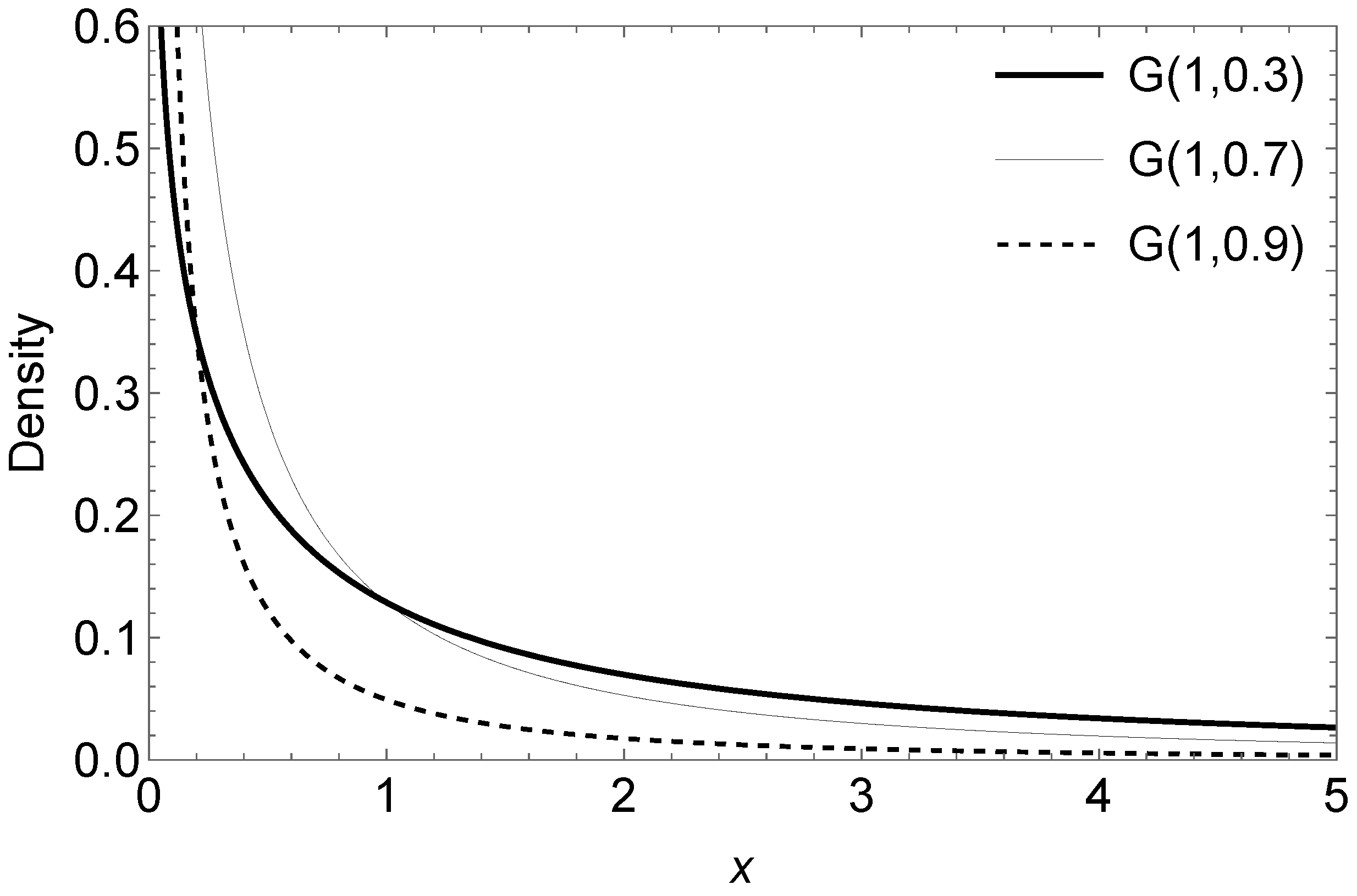
In this section, we study the basic properties of the G distribution given in (4) incorporating a scale parameter. A random variable X has a G distribution with positive support and parameters $\sigma$ and $\alpha$ if its pdf is:

$$f_X(x;\sigma ,\alpha )=\frac{{\sigma }^{\alpha }{x}^{-\alpha }}{B(\overline{\alpha },\alpha )(\sigma +x)},x>0,$$

(5)

where $\sigma >0$ scale parameter and $0<\alpha <1$ shape parameter; we denote this by $X\sim G(\sigma ,\alpha )$. The G distribution is an alternative model to distributions with two parameters, to be used for modelling actuarial statistics data such as the Pareto and GHN distributions, among others. Figure 1 shows the graph of the G density for different values of parameter $\alpha$, fixing $\sigma =1$.

We perform a brief comparison illustrating that the tails of the G distribution are heavier when the $\alpha$ parameter decreases.

Table 1. Tails comparison.

Distribution	$\mathit{P}(\mathit{X}>2)$	$\mathit{P}(\mathit{X}>3)$	$\mathit{P}(\mathit{X}>4)$
G(1, 0.9)	$0.04803$	$0.03537$	$0.02818$
G(1, 0.7)	$0.19065$	$0.15106$	$0.12697$
G(1, 0.3)	$0.63376$	$0.57717$	$0.53760$

shows $P(X>x)$ for different values of x in this distribution.

2.1. Properties

The following proposition shows some properties of the G distribution.

Proposition 1. 

Let $X\sim G(\sigma ,\alpha )$ and $Y\sim Beta(1-\alpha ,\alpha )$. Then,

(a) 

the G distribution has unimodality (at 0).

(b) 

$\frac{\sigma Y}{1-Y}\sim G(\sigma ,\alpha )$.

(c) 

the cumulative distribution function (cdf) of X is given by

$$F_X(x;\sigma ,\alpha )=I_y\left(\overline{\alpha },\alpha \right),x>0,$$

(6)

where $y=\frac{x}{\sigma +x}$ and $I_y(·,·)$ is the regularised incomplete beta function.

(d) 

the hazard function of X is decreasing for all $x>0$.

(e) 

the r-th moment of the random variable X does not exist for $r\ge \alpha$.

(f) 

$\frac{1}{1+X}\sim Beta(\alpha ,\overline{\alpha }).$

(g) 

the quantile function (Q) of the G distribution is given by

$$\begin{array}{c}\hfill Q\left(p\right)=\frac{\sigma I_p^{-1}(\overline{\alpha },\alpha )}{1-I_p^{-1}(\overline{\alpha },\alpha )},0<p<1,\end{array}$$

(7)

where $I_p^{-1}$ is the inverse function of the regularised incomplete beta function.

Proof. 

(d) Using the theorem, item (b), given in Glaser [19] we have that

$$\begin{array}{c}\hfill \eta \left(x\right)=-\frac{f_X^{\prime }(x;\sigma ,\alpha )}{f_X(x;\sigma ,\alpha )}=\frac{\alpha }{x}+\frac{1}{\sigma +x},\end{array}$$

where $f_X(x;\sigma ,\alpha )$ is the pdf given in (5), then the derivative of $\eta \left(x\right)$ with respect to x

$$\begin{array}{c}\hfill {\eta }^{\prime }\left(x\right)=-\left(\frac{\alpha }{x^2}+\frac{1}{{(\sigma +x)}^2}\right)<0,\forall x>0\end{array}$$

gives the result.

(e) 

Considering $\sigma =1$, we claim that the integral ${\int }_1^{\infty }\frac{x^{-\alpha +r}}{1+x}dx$ is divergent.

In fact, taking $g_1\left(x\right)=\frac{x^{-\alpha +r}}{1+x}$ and $g_2\left(x\right)=\frac{1}{x^{1+\alpha -r}}$, we have that

$${\displaystyle \underset{x\to \infty }{lim}\frac{g_1\left(x\right)}{g_2\left(x\right)}=\underset{x\to \infty }{lim}\frac{x}{1+x}=1\ne 0;}$$

and as the integral ${\int }_1^{\infty }\frac{1}{x^{1+\alpha -r}}dx$ is divergent for $r\ge \alpha$ this proves the claim.

On the other hand, since $\mathbb{E}\left(X^r\right)=\frac{1}{B(\overline{\alpha },\alpha )}{\int }_0^{\infty }\frac{x^{-\alpha +r}}{1+x}dx$, by using comparison

$$0\le {\int }_1^{\infty }\frac{x^{-\alpha +r}}{1+x}dx\le {\int }_0^{\infty }\frac{x^{-\alpha +r}}{1+x}dx,$$

and the above claim, the result is reached.

     □

The survival function $\overline{F}\left(t\right)$, which is the probability that an item will not fail before time t, is defined by $\overline{F}\left(t\right)=1-F\left(t\right)$. The survival function for a G random variable is given by $\overline{F}\left(t\right)=1-I_{t/(\sigma +t)}\left(\overline{\alpha },\alpha \right)$.

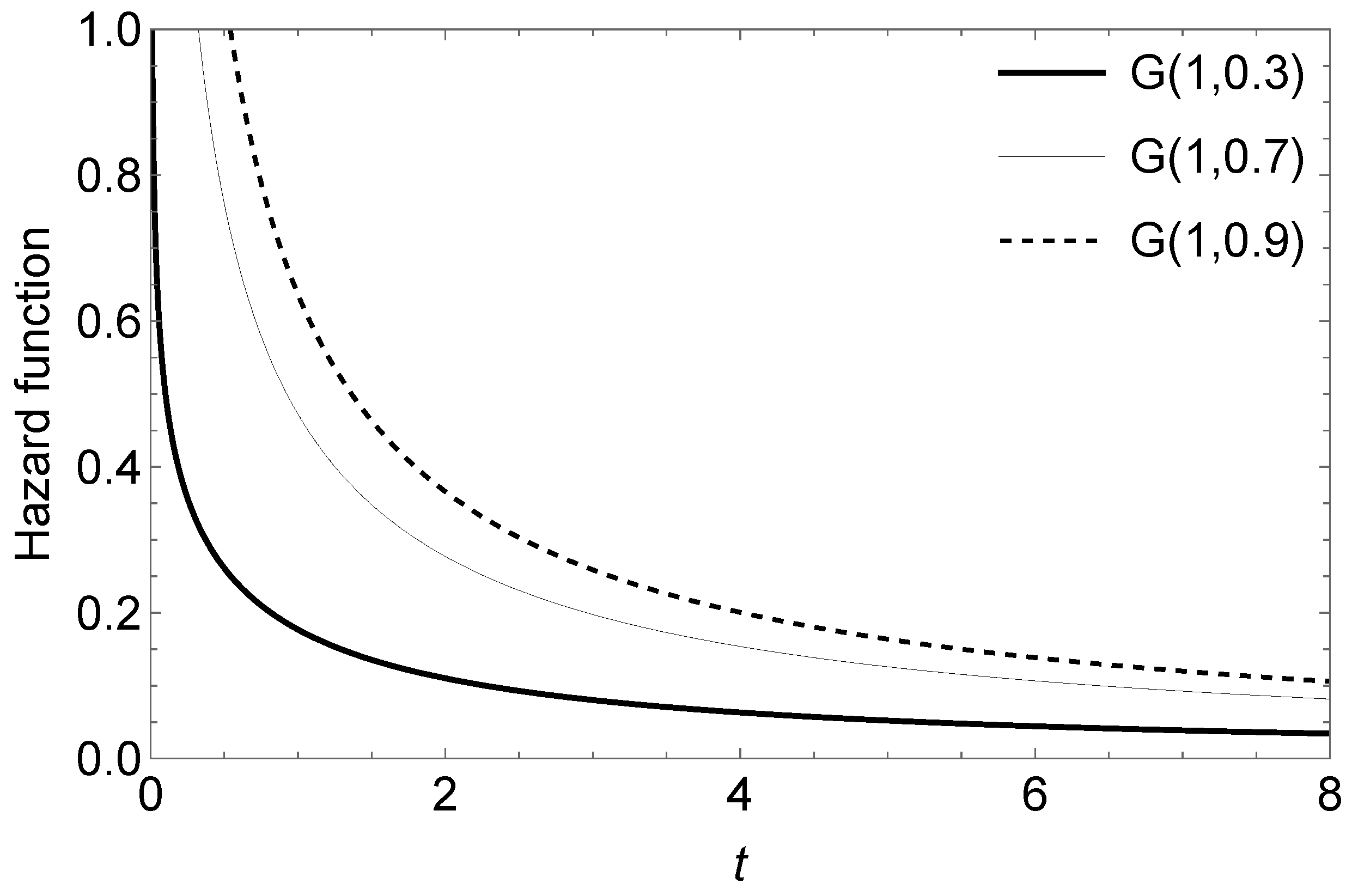
The hazard function $h\left(t\right)$, defined by $h\left(t\right)=\frac{f\left(t\right)}{\overline{F}\left(t\right)}$, for a G random variable is given by

$$\begin{array}{c}\hfill h\left(t\right)=\frac{{\sigma }^{\alpha }{t}^{-\alpha }}{(\sigma +t)\left(B(\overline{\alpha },\alpha )-B\left(\frac{t}{\sigma +t},\overline{\alpha },\alpha \right)\right)},t>0.\end{array}$$

Figure 2 shows the form of the hazard function for different values of $\alpha$, considering $\sigma =1$. As we show in Proposition 1, part $\left(d\right)$, the hazard function is always a decreasing function. In the context of reliability, it indicates that failures are more likely to occur earlier in a product’s useful life.

Using the $Q\left(p\right)$ function given in Proposition 1$\left(g\right)$, we can compute the coefficient of skewness ($\sqrt{{\beta }_1}$) and the coefficient of kurtosis (${\beta }_2$) for the random variable $X\sim G(\sigma ,\alpha )$

$$\sqrt{{\beta }_1}=\frac{Q\left(\frac{3}{4}\right)+Q\left(\frac{1}{4}\right)-2Q\left(\frac{2}{4}\right)}{Q\left(\frac{3}{4}\right)-Q\left(\frac{1}{4}\right)},{\beta }_2=\frac{Q\left(\frac{3}{8}\right)-Q\left(\frac{1}{8}\right)+Q\left(\frac{7}{8}\right)-Q\left(\frac{5}{8}\right)}{Q\left(\frac{3}{4}\right)-Q\left(\frac{1}{4}\right)}.$$

Figure 3 depicts plots for the skewness and kurtosis coefficients in the G distribution.

2.2. Actuarial Measure

The value at risk (VaR) is used to assess the risk exposure, i.e., it can be used to determine the amount of capital necessary to liquidate adverse results. The VaR of the random variable $X\sim G(\sigma ,\alpha )$ is defined as (see Artzner [20] and Artzner et al. [21])

$$Va{R}_p=Q\left(p\right)=\frac{\sigma I_p^{-1}(\overline{\alpha },\alpha )}{1-I_p^{-1}(\overline{\alpha },\alpha )},0<p<1,$$

where $I_p^{-1}$ is the inverse function of the regularised incomplete beta function.

Figure 4 shows graphs of the VaR${}_p$ measurement of distribution G($10,\alpha$) for different values of parameter $\alpha$. We may observe that the smaller the value of parameter $\alpha$, the larger the value of the VaR${}_p$ measurement.

2.3. Order Statistics

Let $X_1,\dots ,X_n$ be a random sample of the random variable $X\sim G(\sigma ,\alpha )$, let us denote by $X_{\left(j\right)}$ the $jth$—order statistics, $j\in \{1,\dots ,n\}$.

Proposition 2. 

The pdf of $X_{\left(j\right)}$ is

$$\begin{array}{c}\hfill f_{X_{\left(j\right)}}(x;\sigma ,\alpha )={\displaystyle \frac{n!}{(j-1)!(n-j)!}}\frac{{\sigma }^{\alpha }{x}^{-\alpha }}{B(\overline{\alpha },\alpha )(\sigma +x)}{\left. [I_{x/(\sigma +x)}(\overline{\alpha },\alpha )\right]}^{j-1}{\left. [1-I_{x/(\sigma +x)}(\overline{\alpha },\alpha )\right]}^{n-j},\end{array}$$

where $x>0$. In particular, the pdf of the minimum, $X_{\left(1\right)}$, is

$$f_{X_{\left(1\right)}}(x;\sigma ,\alpha )=\frac{n{\sigma }^{\alpha }{x}^{-\alpha }}{B(\overline{\alpha },\alpha )(\sigma +x)}{\left. [1-I_{x/(\sigma +x)}(\overline{\alpha },\alpha )\right]}^{n-1},x>0$$

(8)

and the pdf of the maximum, $X_{\left(n\right)}$, is

$$f_{X_{\left(n\right)}}(x;\sigma ,\alpha )=\frac{n{\sigma }^{\alpha }{x}^{-\alpha }}{B(\overline{\alpha },\alpha )(\sigma +x)}{\left. [I_{x/(\sigma +x)}(\overline{\alpha },\alpha )\right]}^{n-1},x>0.$$

Proof. 

Since we are dealing with an absolutely continuous model, the pdf of the $jth$—order statistics is obtained by applying

$$f_{X_{\left(j\right)}}(x;\sigma ,\alpha )={\displaystyle \frac{n!}{(j-1)!(n-j)!}}{f}_X(x;\sigma ,\alpha ){\left[F_X(x;\sigma ,\alpha )\right]}^{j-1}{[1-F_X(x;\sigma ,\alpha )]}^{n-j},j\in \{1,\dots ,n\}$$

where F and f denote the cdf and pdf of the parent distribution, $X\sim G(\sigma ,\alpha )$ in this case.    □

2.4. Entropy

In this subsection we will discuss the Shannon and Rényi entropies of the G model.

2.4.1. Shannon Entropy

The following lemma will be very useful for calculating the Shannon entropy.

Lemma 1. 

Let $X\sim G(\sigma ,\alpha )$, then we have the following results.

1. 

$\mathbb{E}\left(\log X\right)=log\sigma +\psi \left(\overline{\alpha }\right)-\psi \left(\alpha \right),$

2. 

$\mathbb{E}\left(\log \right(\sigma +X\left)\right)=log\sigma -\gamma -\psi \left(\alpha \right),$

where $\psi (·)$ is the digamma function and $\gamma =-\psi \left(1\right)$ is Euler’s constant.

Proof. 

Both results are obtained directly using the pdf given in (5).    □

The Shannon (S) entropy (see Shannon [22]) for a random variable X is defined as

$$S\left(X\right)=-\mathbb{E}\left(\log f_X\left(X\right)\right).$$

(9)

Therefore, it can be verified that the S entropy for the G model is

Proposition 3. 

Let $X\sim G(\sigma ,\alpha )$. Then the Shannon entropy of X is

$$S\left(X\right)=log\sigma +logB(\overline{\alpha },\alpha )-\gamma +\alpha \psi \left(\overline{\alpha }\right)-(1+\alpha )\psi \left(\alpha \right).$$

(10)

Figure 5 shows the Shannon entropy for the G model fixing $\sigma =1$.

2.4.2. Rényi Entropy

A generalization of the Shannon entropy is the Rényi ($R_p$) entropy, which is defined as

$$R_p\left(X\right)=\frac{1}{1-p}log\left({\int }_0^{\infty }{\left[f_X\left(x\right)\right]}^{p}dx\right).$$

(11)

Therefore, it can be verified that the $R_p$ entropy for the G model is

Proposition 4. 

Let $X\sim G(\sigma ,\alpha )$. Then the Rényi entropy of X is

$$R_p\left(X\right)=\frac{1}{1-p}\left(\log \mathsf{\Gamma }\left(\xi \right)+log\mathsf{\Gamma }(p-\xi )-log\mathsf{\Gamma }\left(p\right)-(p-1)log\sigma -plogB(\overline{\alpha },\alpha )\right),$$

(12)

where $\xi =1-p\alpha >0.$

Corollary 1. 

Let $X\sim G(\sigma ,\alpha )$ with $S\left(X\right)$ and $R_p\left(X\right)$ the Shannon and Rényi entropies. Then we have

$$\underset{p\to 1}{lim}{R}_p\left(X\right)=S\left(X\right).$$

(13)

3. Tail of the Distribution

A random variable with a non-negative support, like the classic Pareto distribution, is commonly used in insurance contexts to model the amount of losses. The size of the distribution tail is fundamental if we want the chosen model to capture quantities sufficiently removed from the start of the distribution support, i.e., atypical (extreme) values. The concept of heavy tail is fundamental for this and other financial scenarios.

The use of heavy right-tailed distributions is of vital importance in general insurance. Pareto, Log-normal and Weibull distributions, among others, have been used to model third party liability insurance losses for motor vehicles, re-insurance and catastrophe insurance.

Let $\mathcal{S}$ be the class of subexponential distributions. That is, $F\in \mathcal{S}$ defined in ${\mathbb{R}}_{+}$ satisfies that:

$$\begin{array}{c}\hfill \underset{x\to \infty }{lim}\frac{1-F^{\ast 2}\left(x\right)}{1-F\left(x\right)}=2,\end{array}$$

where $F^{\ast j}$ is the j-fold convolution of F.

The following Lemma, appearing, among others, in  Chapet 2, p. 55 in  Rolski et al. [23], is required in the next Theorem.

Lemma 2. 

Let $F\left(x\right)$ and $H\left(x\right)$ be two distributions on ${\mathbb{R}}_{+}$ and assume that there exists a constant $c>0$ such that

$$\begin{array}{c}\hfill \underset{x\to \infty }{lim}\frac{\overline{H}\left(x\right)}{\overline{F}\left(x\right)}=c.\end{array}$$

(14)

Then, $F\in \mathcal{S}$ if and only if $H\in \mathcal{S}$.

Theorem 1. 

Let the cdf of $G(\sigma ,\alpha )$ given in (6). Then, $F_X(x;\sigma ,\alpha )\in \mathcal{S}$.

Proof. 

Let ${\overline{H}}_X(x;\sigma ,\alpha )={(\sigma /(\sigma +x))}^{\alpha }$ the survival function of the Pareto Type II distribution (Lomax distribution). By using this together with the complementary of the cdf (6) and by computing (14) we get, after applying L’Hopital’s rule, that

$$\begin{array}{c}\hfill \underset{x\to \infty }{lim}\frac{\overline{H}\left(x\right)}{\overline{F}\left(x\right)}=\alpha B(\overline{\alpha },\alpha )>0.\end{array}$$

Now, taking into account that the Pareto type II distribution belongs to the class of subexponential distributions, we have the result.    □

As a consequence of the previous Theorem (see Rolski et al. [23] p. 50), we have the following Corollary.

Corollary 2. 

If $X_1$ and $X_2$ are independent and identically distributed random variables with distributions given in (6), then as $x\to \infty$

$$\begin{array}{c}\hfill Pr(X_1+X_2>x)\sim Pr(\max \{X_1,X_2\}>x).\end{array}$$

Proof. 

The result is a consequence of the fact that $F_X(x;\sigma ,\alpha )\in \mathcal{S}$.    □

Proposition 5. 

It is verified that $F_X(x;\sigma ,\alpha )$ is heavy right-tailed distribution.

Proof. 

Since $F_X(x;\sigma ,\alpha )\in \mathcal{S}$, the result is a consequence of applying Theorem 2.5.2 in Rolski et al. [23].    □

Another way to see that $F_X(x;\sigma ,\alpha )$ is a heavy right-tailed distribution is by computing the limit ${lim}_{x\to \infty }(-log{\overline{F}}_X(x;\sigma ,\alpha )/x)$, which results 0. Observe that $-log{\overline{F}}_X(x;\sigma ,\alpha )/x)$ is the hazard function of X.

As a consequence of the last result, we have the following Corollary:

Corollary 3. 

It is verified that $lim{sup}_{x\to \infty }{e}^{sx}{\overline{F}}_X(x;\sigma ,\alpha )=\infty$, $s>0$.

In this case the distribution fails to possess any positive exponential moment, i.e., $\int exp\left(sx\right)d{F}_X(x;\sigma ,\alpha )=\infty$ for all $s>0$ see Chapter 1, p. 2 [24]. Distributions of this type have moment generating function $M_{F_X(x;\sigma ,\alpha )}\left(s\right)=\infty$, for all $s>0$. This occurs, for example, with the log-normal distribution.

An important issue in extreme value theory is regular variation (see Bingham [25] and Konstantinides [26]). This is a flexible description of the variation of some functions according to the polynomial form of the type $x^{-\delta }+o\left(x^{-\delta }\right)$, $\delta >0$. This concept is formalized in the following definition.

Definition 1. 

A CDF (measurable function) is called regular varying at infinity with index $-\delta$ if it holds:

$$\begin{array}{c}\hfill \underset{x\to \infty }{lim}\frac{\overline{F}\left(\tau x\right)}{\overline{F}\left(x\right)}={\tau }^{-\delta },\end{array}$$

where $\tau >0$ and the parameter $\delta \ge 0$ is called the tail index.

The following proposition establishes that the survival function of the G distribution is a distribution with regular variation.

Proposition 6. 

The survival function of $G(\sigma ,\alpha )$ is regularly varying with tail index α.

Proof. 

Applying the above definition and using L’Hopital’s Rule, we have that

$$\underset{x\to \infty }{lim}\frac{\overline{F}\left(tx\right)}{\overline{F}\left(x\right)}=t^{-\alpha +1}\underset{x\to \infty }{lim}{\left(\frac{\sigma +x}{\sigma +tx}\right)}^{-\alpha }{\left(\frac{\sigma +x}{\sigma +tx}\right)}^{\alpha -1}{\left(\frac{\sigma +x}{\sigma +tx}\right)}^2=t^{-\alpha +1}\underset{x\to \infty }{lim}\frac{\sigma +x}{\sigma +tx},$$

Calculating the limit to the right, we obtain the result.    □

In actuarial settings and individual and collective risk models, the practitioner is usually interested in the random variable $S_n={\sum }_{i=1}^n{X}_i$ for $n\ge 1$. Although its pdf is difficult or impossible to calculate in practice, we can approximate its probabilities using the following Corollary (see Jessen and Mikosch [27]).

Corollary 4. 

If $X_1,\dots ,X_n$ are iid random variables $G(\sigma ,\alpha )$ and $S_n={\sum }_{i=1}^n{X}_i,n\ge 1$, then

$$\begin{array}{c}\hfill Pr(S_n>x)\sim nPr(X_1>x),asx\to \infty .\end{array}$$

(15)

Therefore, if $P_n={max}_{i=1,\dots ,n}{X}_i,n\ge 1$, we have that

$$\begin{array}{c}\hfill Pr(S_n>x)\sim nPr(X>x)\sim Pr(P_n>x).\end{array}$$

This means that for large x the event $\{S_n>x\}$ is due to the event $\{P_n>x\}$. Therefore, high thresholds being exceeded by the sum $S_n$ are due to this threshold being exceeded by the largest value in the sample.

As Jessen and Mikosch [27] point out, expression (15) can be taken as the definition of a subexponential distribution. The class of those distributions is larger than the class of regularly varying distributions. The result, given in Corollary 4, remains valid for subexponential distributions because the subexponentiality of $S_n$ implies subexponentiality of $X_1$. Usually, this property is referred to as convolution root closure of subexponential distributions. More details can be viewed in [28,29].

On the other hand, let the random variable X, whose support is $0<x<\infty$, represents either a policy limit or reinsurance deductible (from an insurer’s perspective); then the limited expected value function L of X with cdf $F\left(x\right)$, is defined by (see Boland [30] and Hogg and Klugman [31]):

$$\begin{array}{c}\hfill L\left(x\right)=\mathbb{E}\left[\min (X,x)\right]={\int }_0^{x}ydF\left(y\right)+x\overline{F}\left(x\right),\end{array}$$

which is the expectation of the cdf $F\left(x\right)$ truncated at this point. In other words, it represents the expected amount per claim retained by the insured on a policy with a fixed amount deductible of x. Observe that we integrate according to the interval $(0,x)$.

Proposition 7. 

Let X be a random variable following the pdf (5). Then the limited expected value of X is given by

$$\begin{array}{c}\hfill L\left(z\right)=\frac{z^2}{\sigma B(\overline{\alpha },\alpha )(2-\alpha )}{\left(\frac{\sigma }{z}\right)}^{\alpha }{}_2{F}_1(2-\alpha ,1,3-\alpha ,-z/\sigma )+z\overline{F}\left(z\right),\alpha <1,\end{array}$$

where ${}_2{F}_1$ represents the hypergeometric function.

Proof. 

By making the change of variable $t=x/(z-x)$ in the integral

$$\begin{array}{c}\hfill I=\frac{{\sigma }^{\alpha }}{B(\overline{\alpha },\alpha )}{\int }_0^z\frac{dx}{x^{\alpha -1}(\sigma +x)},\end{array}$$

gives the result.    □

4. Inference

In this section we estimate the parameters of the G model by the ML method, and discuss a simulation study and asymptotic estimation of the ML estimators.

4.1. ML Estimation

For a random sample $x_1,\dots ,x_n$ derived from the $G(\sigma ,\alpha )$ distribution, the log-likelihood function can be written as

$$\ell (\sigma ,\alpha )=n\alpha log\sigma -\alpha \sum _{i=1}^{n}log{x}_i-nlogB(\overline{\alpha },\alpha )-\sum _{i=1}^{n}log(\sigma -x_i).$$

(16)

The score equations are given by:

$$\begin{array}{c}\hfill \frac{n\alpha }{\sigma }-\sum _{i=1}^n\frac{1}{\sigma +x_i}=0,\end{array}$$

(17)

$$\begin{array}{c}\hfill log\sigma -\overline{logx}+\psi (1-\alpha )-\psi \left(\alpha \right)=0,\end{array}$$

(18)

where $\psi (·)$ is the digamma function and $\overline{logx}=\frac{1}{n}{\sum }_{i=1}^{n}log{x}_i$. From (17) we obtain

$$\begin{array}{c}\hfill \widehat{\alpha }=\frac{\widehat{\sigma }}{n}\sum _{i=1}^n\frac{1}{\widehat{\sigma }+x_i},\end{array}$$

(19)

and the ML estimator for $\sigma$ ($\widehat{\sigma }$) is obtained by solving numerically the following equation

$$\begin{array}{c}\hfill log\widehat{\sigma }=\overline{logx}+\psi \left(\frac{\widehat{\sigma }}{n}\sum _{i=1}^n\frac{1}{\widehat{\sigma }+x_i}\right)-\psi \left(1-\frac{\widehat{\sigma }}{n}\sum _{i=1}^n\frac{1}{\widehat{\sigma }+x_i}\right).\end{array}$$

(20)

Equation (20) can be solved by using numerical procedures such as the Newton-Raphson algorithm. Alternatively, these estimates can be found by directly maximizing the log-likelihood surface given by (16) and using the “optim” subroutine in the R software package [32] version 4.2.1.

4.2. Simulation Study

To examine the behaviour of the ML estimation, we present a simulation study to evaluate its performance, evaluating the $\sigma$ and $\alpha$ parameters in the G model. The simulation was analysed by generating 1000 samples of size $n=100,$ 200 and 500 from the G model. The object of this simulation was to study the behaviour of the ML of the G model parameters. Algorithms 1 and 2 can be used to generate random numbers from the G model, as shown below.

Algorithm 1 For simulating from the $X\sim G(\sigma ,\alpha )$ can proceed as follows

Step 1: Generate $Y\sim Uniform(0,1).$ Step 2: Compute $X=\frac{\sigma I_Y^{-1}(\overline{\alpha },\alpha )}{1-I_Y^{-1}(\overline{\alpha },\alpha )}$.

Algorithm 2 For simulating from the $X\sim G(\sigma ,\alpha )$ can proceed as follows

Step 1: Generate $Y\sim Beta(\overline{\alpha },\alpha ).$ Step 2: Compute $X=\frac{\sigma Y}{1-Y}$.

For each sample generated from the G distribution, the ML estimates are obtained by applying the Newton-Raphson algorithm. In

Table 2. Empirical bias, SE, RMSE and 95% CP for the ML estimators of $\sigma$ and $\alpha$ in the G distribution with different combinations of parameters.

True Value			$\mathit{n}=100$				$\mathit{n}=200$				$\mathit{n}=500$
$\mathit{\sigma }$	$\mathit{\alpha }$	Par.	Bias	SE	RMSE	CP	Bias	SE	RMSE	CP	Bias	SE	RMSE	CP
1	0.2	$\sigma$	0.1934	0.5709	0.6543	0.9402	0.1113	0.3727	0.4083	0.9474	0.0494	0.2219	0.2292	0.9540
		$\alpha$	0.0054	0.0260	0.0270	0.9618	0.0039	0.0181	0.0186	0.9562	0.0022	0.0113	0.0116	0.9542
	0.5	$\sigma$	0.2191	0.7544	0.8668	0.9004	0.1006	0.4920	0.5425	0.9156	0.0468	0.3010	0.3131	0.9370
		$\alpha$	0.0004	0.0679	0.0667	0.9258	$-0.0012$	0.0496	0.0491	0.9308	0.0005	0.0322	0.0320	0.9424
	0.8	$\sigma$	0.0727	0.5090	0.5498	0.8988	0.0348	0.3463	0.3602	0.9216	0.0118	0.2137	0.2143	0.9432
		$\alpha$	$-0.0044$	0.0258	0.0271	0.9550	$-0.0022$	0.0179	0.0183	0.9496	$-0.0010$	0.0112	0.0114	0.9510
10	0.2	$\sigma$	1.9401	5.7013	6.4320	0.9394	1.1103	3.7292	4.0676	0.9486	0.4651	2.2140	2.2556	0.9528
		$\alpha$	0.0052	0.0260	0.0268	0.9562	0.0037	0.0181	0.0189	0.9492	0.0020	0.0113	0.0112	0.9560
	0.5	$\sigma$	1.9611	7.4418	8.4714	0.8872	1.0610	4.9654	5.2373	0.9176	0.4148	2.9938	3.0764	0.9360
		$\alpha$	$-0.0014$	0.0681	0.0668	0.9216	0.0002	0.0497	0.0490	0.9344	0.0000	0.0322	0.0315	0.9484
	0.8	$\sigma$	0.6832	5.0843	5.3895	0.8952	0.3724	3.4679	3.5625	0.9236	0.1692	2.1465	2.1721	0.9406
		$\alpha$	$-0.0047$	0.0259	0.0274	0.9510	$-0.0020$	0.0179	0.0181	0.9544	$-0.0008$	0.0112	0.0113	0.9534

the empirical bias, the mean of the standard errors (SE), the root of the empirical mean squared error (RMSE), and the 95% coverage probability (CP) based on the asymptotic distribution for ML estimators are given for the estimators of the parameters. As Table 2 shows, the performance of the estimates improves when n increases.

4.3. Fisher’s Information Matrix

Let us now consider $X\sim G(\sigma ,\alpha )$. For a single observation x of X, the log-likelihood function for $\mathbf{\theta }=(\sigma ,\alpha )$ is given by

$$\ell \left(\mathbf{\theta }\right)=\alpha log\sigma -\alpha logx-logB(\overline{\alpha },\alpha )-log(\sigma +x).$$

The corresponding first and second partial derivatives of the log-likelihood function are derived in Appendix A. It can be shown that the Fisher’s information matrix, denoted by $I_F(·)$, for the G distribution is provided by

$$I_F\left(\mathbf{\theta }\right)=\left(\begin{array}{cc}\frac{\overline{\alpha }\alpha }{2{\sigma }^2}& -\frac{1}{\sigma }\\ -\frac{1}{\sigma }& {\psi }^{\prime }\left(\alpha \right)+{\psi }^{\prime }\left(\overline{\alpha }\right)\end{array}\right),$$

where ${\psi }^{\prime }(·)$ is the trigamma function.

Proposition 8. 

The ML estimate of θ is consistent and asymptotically normal, verifying

$$\sqrt{n}\left(\widehat{\theta }-\theta \right)\stackrel{\mathcal{L}}{⟶}{N}_2(\mathbf{0},I_F{\left(\theta \right)}^{-1}),asn\to \infty .$$

Proof. 

The distribution satisfies the regularity conditions see Lehmann and Casella [33] p. 449 under which the ML estimator $\widehat{\theta }$ of $\theta$ is consistent and asymptotically normal. □

Thus the asymptotic variance of the ML estimator $\widehat{\theta }$ is the inverse of Fisher’s information matrix $I_F\left(\theta \right)$. Since the parameters are unknown, the observed information matrix is usually considered, where the unknown parameters are estimated by ML.

5. Applications

In this section we analyse two applications, the first with simulated data and the second with real data. To compare the models, we use the Akaike information criterion AIC (see Akaike [34]) and the Bayesian information criterion BIC (see Schwarz [35]). In these applications we use the GHN model (see Cooray and Ananda [36]) and the Pareto model (see Arnold [37]). These models present a certain similarity in form with the G model and have greater flexibility in their coefficient of kurtosis. Hence the Pareto and GHN models are considered in the comparison of the fits to the two data sets. The two models are given respectively by:

• $f(x;\alpha ,\beta )=\frac{\beta {\alpha }^{\beta }}{x^{\beta +1}},x>\alpha ,$
• $f(x;\sigma ,\alpha )=\frac{2\alpha x^{\alpha -1}}{{\sigma }^{\alpha }}\varphi \left({\left(\frac{x}{\sigma }\right)}^{\alpha }\right),x>0,$

where $\varphi$ denotes the density function of the standard normal distribution and $\sigma ,\alpha ,\beta >0$.

5.1. Numerical Application

In this numerical application we analyse 200 simulated data generated from the G($1,0.3$) model using Algorithm 1 given in Section 4.2. The object of this numerical example is to use the ML method given in Section 4.1 to see whether, when the G model is fitted, it has its own form.

Table 3. 200 simulated data: Model, ML estimates, AIC and BIC values.

Model	ML Estimates	AIC	BIC
G($\sigma ,\alpha$)	$\widehat{\sigma }=0.890$, $\widehat{\alpha }=0.295$	1967.556	1974.152
Pareto($\alpha ,\beta$)	$\widehat{\alpha }=0.002$, $\widehat{\beta }=0.121$	2144.958	2151.555
GHN($\sigma ,\alpha$)	$\widehat{\sigma }=204.871$, $\widehat{\alpha }=0.144$	2143.358	2151.787

shows the ML estimates for the parameters of the G model, Pareto model and GHN model, as well as the AIC and BIC values for each model.

We observe that the smallest values of the AIC and BIC criteria correspond to the G model, meaning that the G model fits the data better than the other models. This is to be expected, since the data were simulated from the G model. The above values for the measures indicate that the G model has its own form and that it may be difficult to replace it by any other known two-parameter model.

5.2. Application with Real Data

This dataset comes from the Survey of Consumer Finances (SCF), a nationally representative sample that contains extensive information on assets, liabilities, income, and demographic characteristics of those sampled (potential U.S. customers). It contains a random sample of 500 households in USA with positive incomes that were interviewed in the 2004 survey. The variable of interest is the annual income of the family in thousands of US dollars divided by the number of members in the household. The data can be recovered from the web page https://www.federalreserve.gov/econres/scfindex.htm (accessed on 5 January 2022). The descriptive statistics of these data are shown in

Table 4. Descriptive statistics for income data.

n	Median	Mean	Variance	CS	CK
500	21.125	216.709	11,270,001	0.435	1.655

, where CS is the coefficient of skewness of the sample and CK is the coefficient of kurtosis of the sample.

Figure 6 presents two boxplot graphs; the left boxplot shows a very extreme datum and the right boxplot shows the dataset after elimination of the extreme datum to show the other extreme data that cannot be seen in the left boxplot. These atypical data make the right tail heavier. It may be noted that the majority of the observations are around 21,125 dollars per capita per family, and there is a very atypical value which is an income of 75 million dollars.

Table 5. ML estimates for the income data with corresponding standard errors (in parentheses), and AIC and BIC values.

Model	ML Estimates	AIC	BIC
G($\sigma ,\alpha$)	$\widehat{\sigma }=21.555\left(6.264\right)$, $\widehat{\alpha }=0.497\left(0.033\right)$	5139.176	5147.605
Pareto($\alpha ,\beta$)	$\widehat{\alpha }=0.065\left(0.001\right)$, $\widehat{\beta }=0.171\left(0.008\right)$	5867.910	5876.339
GHN($\sigma ,\alpha$)	$\widehat{\sigma }=64.313\left(6.815\right)$, $\widehat{\alpha }=0.335\left(0.008\right)$	5280.360	5288.789

shows the ML estimates for the parameters of the G, Pareto and GHN models, as well as the values of the AIC and BIC criteria for each model.

We observe that the smallest values of the AIC and BIC criteria correspond to the G model, meaning that the G model fits the data better than the Pareto and GHN models. The SE of the ML of the G model were calculated using Section 4.1.

Table 6. Comparison of VaR of different models for income data and empirical quantiles in parentheses.

Model∖Significance	0.50 (21.125)	0.60 (28.600)	0.70 (40.000)	0.80 (60.000)	0.90 (100.000)	0.95 (210.250)
G ($\widehat{\sigma },\widehat{\alpha }$)	22.034	41.764	85.060	209.891	889.770	3632.538
Pareto ($\widehat{\alpha },\widehat{\beta }$)	3.744	13.805	74.248	795.165	45800.120	2638007
GHN ($\widehat{\sigma },\widehat{\alpha }$)	19.836	38.426	71.568	134.928	284.355	479.988

presents estimates of the VaR for the G, Pareto, and GHN models at the levels of 0.50, 0.60, 0.70, 0.80, 0.90, and 0.95 and empirical quantiles. It is well known that the models with the highest VaR values have the heaviest tails. Then, based on this characteristic, we can see that the G model has higher VaR values than the GHN model. On the other hand, the G model provides higher VaR values up to the 0.70 level than the Pareto model since the Pareto VaRs explode at high (but not too high) quantiles. Due to the selection criteria of the AIC and BIC models, the G model best fits the income data. Figure 7 shows the behavior of the VaR values of the three models. Figure 8 shows the empirical cdf with estimated G and Pareto cdf’s, which also shows the excellent agreement between the G model and the income data.

6. Discussion

This paper presents a study of the G model, used in a characterization of the gamma distribution. The G model is a special case of the prime beta model with one scale parameter. The G model has two parameters and this makes it an attractive competitor against various two-parameter models used in actuarial statistics. The G model appears to be a viable alternative for fitting data with extreme observations. Some other characteristics of the G model are:

• The smaller parameter $\alpha$, the heavier the right tail of the G model.
• The G model has an explicit representation given in Proposition 1 $\left(b\right)$.
• Cdf, risk function and quantile function are explicit and are represented by known functions.
• The VaR measurement is explicit and is used to show that the right tail of the G model is heavy.
• The applications show that the G model has its own characteristic compared with other two-parameter models, and that the G model can be a good candidate for modelling income data with a heavy tail.