Abstract
The advancement of technology influenced the development of mechanical and mechatronic systems. This article presents the integration of new technologies into traditional mechanics. Specifically, it presents a flexible interactive software for dynamic plane geometry used for designing, simulating and analyzing the mechanical systems. The article presents this interactive software for dynamic geometry as a useful tool for the kinematic analysis of constrained linkages. The simulation and kinematic analysis of some mechanical systems are presented.
Keywords:
dynamic geometry; geometric loci; dynamic homotopy; trajectories; simulations of mechanical systems; kinematic analysis MSC:
68U05; 68V30; 70B15
1. Introduction
The mechanical systems with rigid body dynamics are modelled by using methods based on the Newtonian laws of motion [1]. However, there are some difficulties in modelling the multibody system; when more mechanical components are interconnected, modelling depends in general on geometry, and simulating these mechanical systems can require a considerable effort [2]. This dependence on geometry requires a special consideration. Since a large class of mechanical systems can be modelled by basic one-dimensional translation and fixed-axis rotation, designing and analyzing mechatronic systems with rather complex mechanical components could be facilitated by a flexible interactive software for dynamic plane geometry. The article presents such an interactive software for dynamic geometry as a tool for engineers and scientists interested in solving kinematic and dynamic problems by using computers. By combining mathematical knowledge and software engineering, this interactive software offers several facilities for geometric loci, trajectories and parametric curves. The dynamic features subsume mobile elements, a path, a direction, speed, acceleration, timing and other parameters. These facilities can simulate dynamic trajectories, complex geometric loci and new geometrical relations. An important aspect is that this software is intuitive and simple to use.
In the first part of this article, we present snapshots exemplifying how the interactive environment is working, particularly on the representation of a curve dynamics with respect to the continuous changes of its parameters. The interactive software for dynamic geometry offers assistance in determining geometrical loci determined by many mobile elements defined by the user. Thus, it is possible to use a geometrical construction, and to indicate the movements of some of its elements. Each movement of an element provides a path given by the mobile element. For example, if the moving element is a point, its corresponding path can be either a line, a curve or a locus. Another option is to select a segment as the moving element, having the segment moving around a point (acting as its path). Another possibility is to have a circle as the moving element and a line as its path; namely, the circle is sliding on the line. If the moving element is a point and the interior of a polygon represents the path, the movement generates a set of arbitrary points inside the polygon. Additional to the mobile element and path, it is allowed to indicate other properties for each movement as direction, speed, change of direction, starting time of the movement (usually 0), a number of repetitions, time of a specific cycle, and a termination time. These properties provide a certain flexibility in playing various simulations, generating a broad spectrum of scenarios in dynamic geometry [3]. By using messages sent by the interactive software, it is possible to check whether some specific geometrical relations and properties are preserved during the whole process. In particular, the correctness of these messages is important when the movement is not possible anymore (because the obtained trajectories in a simulation cannot describe properly the behaviour of a mechanism). For instance, when such a mechanism contains rigid segments (fixed length), it is possible to stop the movement, also emitting a specific warning. Technically, when a critical situation appears, the involved element returns to its previous position, and sends a message to its parent. Such a recovery procedure is applied recursively until all (involved) elements are moved back to their previous positions, and movement is stopped; additionally, an exception identifying the deadlock type is raised.
One possible utilization of the dynamic geometry software is related to the kinematics of mechanical and robotic systems [4]. We present how to use our interactive software to simulate some scenarios in order to design properly mechanical systems by interconnecting several components. Joint constraints capture the interaction among rigid bodies. Using our software, the designer introduces easily the dynamic geometry of the joints, and the software verifies their consistency. The algorithms can extract the parameters for each component, and joint components are computed and instantiated based on the interconnections between components. The mechanical behaviour of each rigid component is described by its position, orientation and the forces acting on the component (velocity, acceleration, variations of the angles and movements). Some conditions are expressed as (linear) algebraic constraints, then converted for simulation. The algorithms can also extract the kinematic behaviour from the resulting geometry. Some possible inconsistencies appear when the kinematic behaviour of the mechanical system does not match the specific geometry properly. We present some examples of designing and simulating mechanical systems by using our flexible software for dynamic geometry, and also providing their kinematic diagrams. The advantage of this software is the intuitive and simple way of describing and simulating the kinematics of mechanical systems.
2. Loci Functionalities
Technically, a trajectory could be used as a path; for this, it is enough to click the trajectory to locate the point as a mobile element. Whenever the selected point (pixel) is not on the trajectory, the closest point of the trajectory is determined (by using a radius decided by the user). Whenever the pixel is very close to the trajectory, the point for the movement appears as being on it (it becomes one of the points of the trajectory). Eventually, we can move (by using the mouse) this point along the trajectory. Whenever an exact fit is not possible, the fitting problem (for a trajectory) is resolved by interpolation and regression analysis (an approximate fit is determined by using a nonlinear regression). Since every plane trajectory can be fairly approximated by a sequence of Bezier curves, the interpolation uses Bernstein polynomials.
When the involved elements move too fast, the distances between captured points of a geometrical locus could be large, and so it could be difficult to determine it properly when only few points (far from each other) are known. Our interactive software allows it to slow down its speed. This aspect is new and indicates a distinctive feature, just because most of the existing software systems present loci functionalities by using a single mobile element without considering its speed.
We exemplify the geometrical loci and trajectories by using some geometric constructions in which the moving elements change their positions according to the path, direction and speed. Moreover, the moving elements can have specific relationships with other involved elements. When a position is changed, certain messages are sent to the other elements placed in the same component vector, namely to the elements involved in a specific geometrical relation. Consequently, the positions of these elements change in such a way so as to preserve the current geometrical relations; this fact leads to a recursive modification of all the components positions. In some situations, the mobile element could appear in the component vector of a different element. Thus, it is possible to have messages asking other changes of its position; sometimes, the movements are not possible. Therefore, it is necessary to manage the messages for each component properly—we name this as the ‘feedback problem’. It is possible to generate several errors, particularly when the geometrical construction is complex. Anyway, once the movements are decided in a correct way, we indicate the elements under observation (they could be many of them). Thus, we set the speed and acceleration for each element, and determine its correct trajectory. Additionally, it is possible to indicate a colour for each trajectory, such that distinct trajectories may be easily observed (by having different colours).

Figure 1.
Example of a simple geometric construction.
Figure 1.
Example of a simple geometric construction.
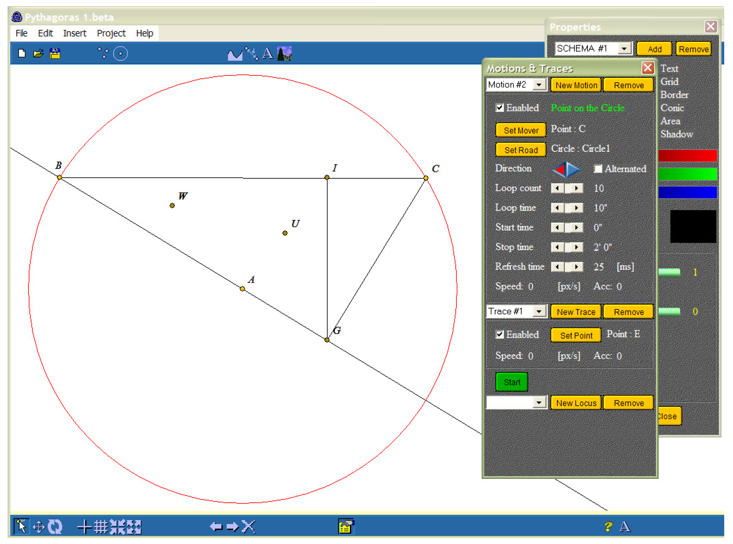
As an example, we consider a rather simple geometric construction (Figure 1) given by a circle and its centre A, together with two points B and C on this circle. We have a line passing through A and B, together with the line perpendicular on AB passing through C (G being the intersection point). Considering the perpendicular passing through G on line BC, its intersection with line BC is denoted by I. The midpoint of line segment AI is denoted by U, and the midpoint of line segment BU is denoted by W. Our interactive software allows it to modify easily (by the mouse) the circle (its position) by moving its centre A as well as its radius. It is easy to change also the positions of B and C moving on the circle. The new obtained points G, I, U, W depends on these geometrical constraints; thus, their positions are not allowed to be changed (by using the mouse). Since line segment CG is perpendicular on line segment AB, it becomes an element of the component vector of line segment AB. Since point G is given by the intersection of lines AB and CG, it belongs to the component vector of both lines. Since line segment GI is perpendicular on BC, it belongs to the component vector of line BC. In a similar way, point I belongs to the component vector of lines BC and GI, point U belongs in both component vectors of points A and I (being the midpoint of AI), and point W belongs to the component vectors of points B and U.
Whenever the position of point B is modified in this construction, a message is sent to its ‘parent’ elements: the circle and line segments BA and BC. Point B does not change the radius (and position) of the circle; in fact, point B represents a rotation point for both BA and BC—this means that it modifies them, and this implies changes for all the elements of the component vectors of BA and BC. Being a rotation point for line segment BA, point A is not affected by changing point B. Since segment CG is in the component vector of line AB (being perpendicular on it), it changes its position and induces the change of point G. Since G is a translation point for GI, line GI modifies its position, as well as the position of I. Point I is also affected because of the movement of segment BC. Since IG belongs to the component vector of segment BC (being perpendicular on it), a change of point I induces a change of point U (related to points I and A), and the changes of points B and U induce a change for W (related to points B and U).
The change of point C triggers less changes in the construction.
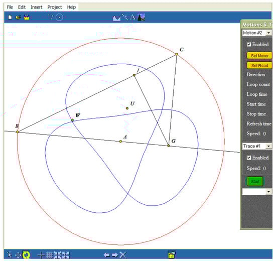
Figure 2.
Trajectory of the point W (its geometrical locus)—adapted from [5].
Figure 2.
Trajectory of the point W (its geometrical locus)—adapted from [5].

We describe all these changes (depicted in Figure 2) in the following way:
Point B - update position;
Line1 - update position; goto et2; Line3 - update position; goto et4;
Point C - update position; goto et2; Line3 - update position; goto et4;
et2: Line2 - update position;
Point G - update position; goto et4;
et4: Line4 - update position;
Point I - update posiTION;
Point U - update posiTION;
Point W - update position;
Two additional movements can be considered in the previous construction. In the first one, we consider point B as a moving element (along the circle). In the second one, we consider point C as a moving element (along the circle); its direction is different, having half of the speed of B. These movements are described in the software by
Motion1: Motion2:
mover: mover:
type: point; type: point;
mover: Point B; mover: Point C;
road: road:
type: circle type: circle
road: Circle1; road: Circle1;
properties: properties:
enabled: true; enabled: true;
direction: clock; direction: inv clock;
alternated: false; alternated: false;
speed: 400 pixel/s; speed: 200 pixel/s;
loop count: 10; loop count: 10;
loop time: 10"; loop time: 10";
start time: 0; start time: 0;
stop time: 2’0"; stop time: 2’0".
Since we associate a thread to each movement, the threads corresponding to points B and C are running concurrently. According to the above description, a change in the position of each point generates a chain of movements. The evolution of point W can be observed in the Figure 2.
In general, it is possible to observe more than one evolution by using the dynamic geometry of this interactive software. Technically, each observation creates a Locus. A thread captures the positions of the observed element with a certain frequency, storing them in a vector associated to its Locus. It is worth noting that the representations of these positions is influenced by the restricted representation of numbers in a computer. Thus, we work with approximations of the correct positions; this means that the approximation errors could be amplified during a simulation.
3. Dynamic Homotopy
Dynamic curves represent one of the new achievements, which could have an important role in education and research. It allows one to create new curves, to manage and edit existent ones, to modify and redraw curves and to use them in the working framework.
It is important to have the visual representation of curve dynamics with respect to changes in parameters. In this system, we can view the changes which occur in the graphic of a curve when one of its parameters is modified. In this way, one can discover particular cases, which would be hard to find without such a feature. The dynamic representation of a curve simulates a homotopy (a continuous deformation) from the initial curve to the modified one. To be more precise, a homotopy from a curve to a curve is a continuous map such that and for all . Simulating a homotopy from to consists of taking discrete ‘snapshots’ of the graphic of , i.e. drawing for some values .
From a technical point of view, the support for manipulating curves is implemented in the comp.gui.curves and comp.gui.curves.parser packages. The data defining a curve is kept in an object of type comp.gui.curves.Curve. The Curve class has the following public fields: name, description, type, min, max, rate, params, x, y, fx, fy and ecurve. Their meaning is presented below:
- name stores the name of the curve;
- description stores its description (its definition and/or some observations);
- type stores the mode of its representation; it can be one of the following: parametric, explicit or polar;
- and store the minimum and maximum values of the argument;
- rate stores the sampling rate;
- params is an object matrix of type comp.gui.curves.Param; each element of this matrix stores the data of one curve parameter, i.e., the name and value of the parameter;
- x and y store the curve equations; for a parametric representation we have and , for an explicit representation, we have and , while for a polar representation x is an angle and y is given by ;
- and have the type comp.gui.curves.parser.Function;
- ecurve is an object of type comp.geom.ECurve, which is used for the graphical representation of the curve.
When calling the methods and , the strings stored in the fields x and y are interpreted, the objects and of type Function (which represent the functions associated to the strings x and y) are built, and the parameters are stored in these objects (which are added in the params matrix). This interpretation takes place whenever there is a redraw request, before using the argument t. The objects and thus created are used for every computation. The methods and return the values of the functions x and y for the parameter t. The methods and are called only at the initial drawing or when the curve is redrawn in the work framework. Other curve operations (editing; saving) do not involve these methods. Therefore, the computation of functions x and y for a parameter t is conducted without interpreting the strings x and y. The objects of the type Curve are created and managed through the graphical interface implemented by the classes MCurves, MCurves1, MCurves2, MCurves3, MCurves4, MCurves41 and MCurves5 from the comp.gui.curves package.
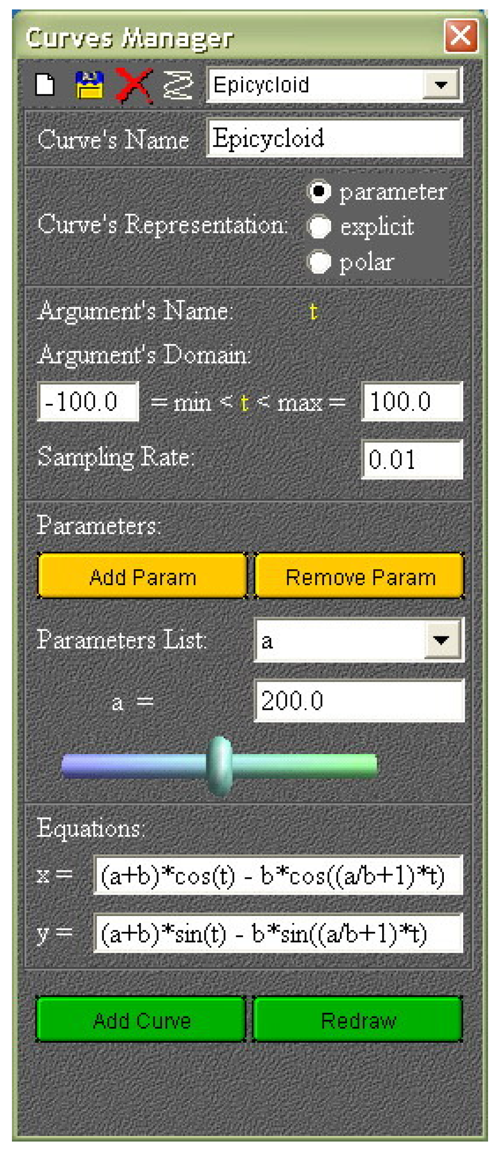
The toolbar buttons of the curve manager allow us to create a new curve, to save it, to erase the current curve, and to switch to the set of famous curves already implemented. In this case, the toolbar list loads depending on the button selected in Curves Representation: when selecting a curve from the list, the editable fields load as in Figure 3.

Figure 3.
Curve manager (toolbar buttons and parameters).
The data of the of famous curves, which are already implemented, are stored in the class comp.gui.curves.Curves. Their equations cannot be edited. To change these equations, the curves must be saved separately and will be sent to the user list. The data for the saved curves is written in a file using a method from the Curves class. This class also provides the means to read curves from this file and to load them in the user list. The contents of this list changes with respect to the active button in the Curves’ Representation. When pressing the AddCurve button, the following happens:
- A curve object from the corresponding Curve object is created and initialized, and it is added to the vector of geometric objects corresponding to the current simulation;
- An object ELocus from the ECurve object is created; it is initialized with the properties set in the property window (colour, size, shadow, and label);
- The method setLocus() from is called. This calls in the methods and from the curve object. Then, by calling methods and of the same object, the coordinates of a specified number of points from the geometrical image of the curve are obtained. These will be loaded in the points vector from the associated ELocus object.
- The redrawing is called, which leads to drawing the ELocus object and thus to the graphical representation of the curve.
The last two steps are executed at every redrawing of the curve. The redrawing is called by changing the value of the current parameter through the scroll bar, or by pressing the ‘redraw’ button. When moving the scroll bar, each value produces a redraw of the current curve, and this simulates a (dynamic) homotopy. The value of the current parameter can also be changed directly. If it is an integer, the scroll changes the parameter with rate 1. If it has one decimal, the scroll changes the parameter with the rate 0.1 and so on.
Examples for Dynamic Geometry
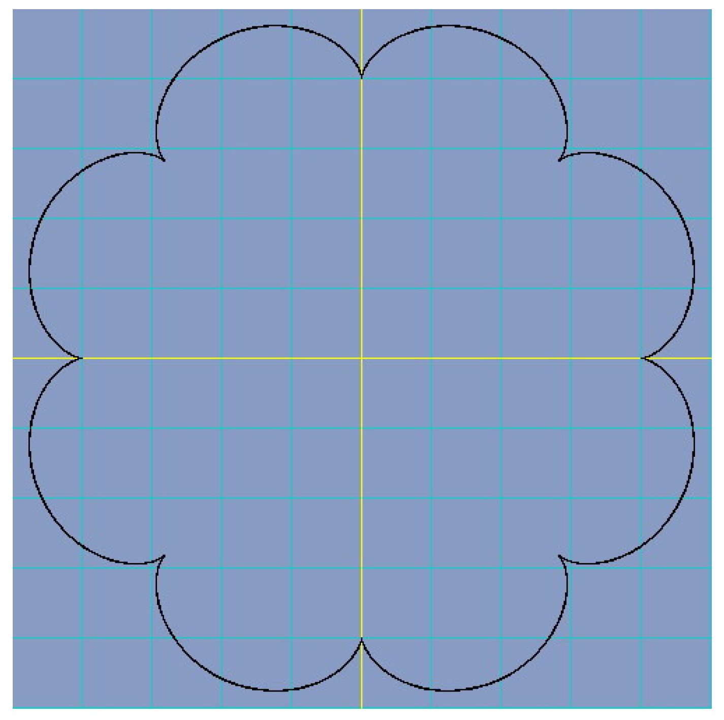
As a first example, we take the Epicycloid, having the equations:
For the values and , when parameter t is varying between 0 and with a rate of , it is graphically represented in Figure 4.
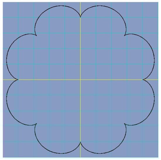
Figure 4.
Epicycloid for values and .
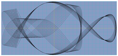
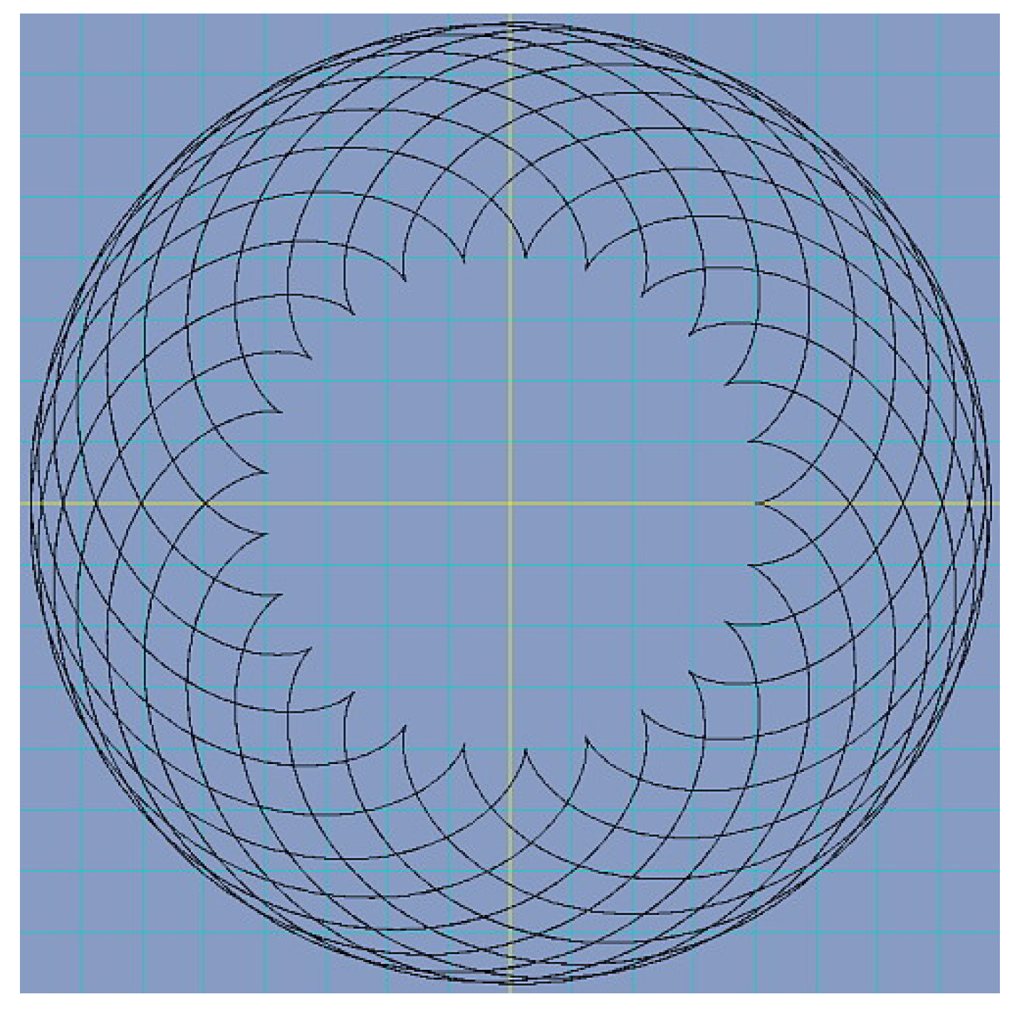
When changing the parameter b to 97, we obtain Figure 5.
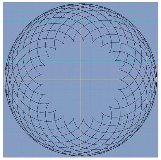
Figure 5.
Epicycloid for values and .
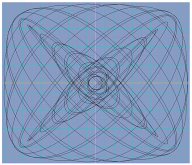
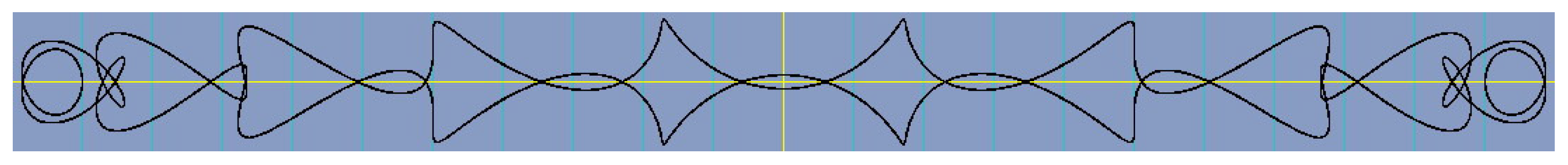
Interesting representations are obtained by slight changes in the curve equations.
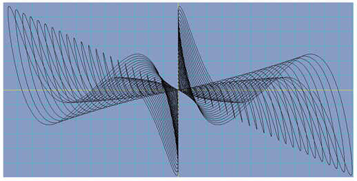
For example, if the equations considered are
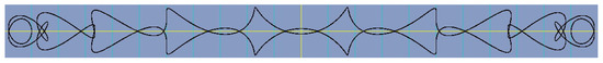
Figure 6.
Epicycloid for values and .
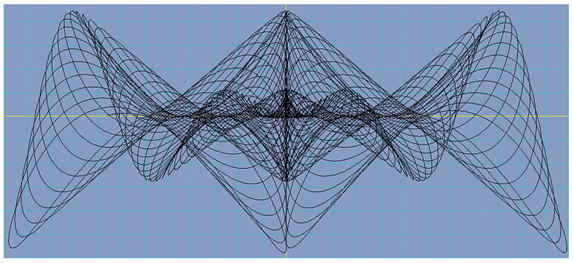
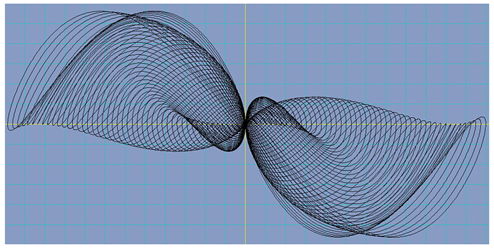
For the equations
We can change the parameter a ‘continuously’ by using the scroll bar, and the above curve changes by also obtaining the following representation for :
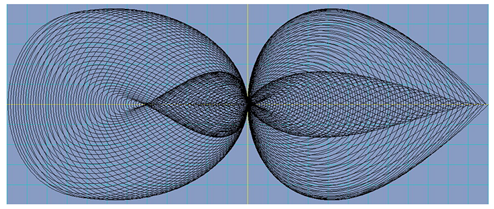
For the equations
For , we obtain the following picture:
For the equations
For we obtain a different graphical representation:
The above examples illustrate the possibilities that are offered by this mathematical software to study the behaviour of plane curves. Unlike other curve drawing programs, it is offered a powerful instrument for studying the curve dynamics with respect to certain parameters. By visualizing homotopies, the researcher can find particular cases, which are hard to imagine in some other way. By parsing the strings that give the curve equations only once, before the initial drawing, i.e., building two objects which represent these formulas, we obtain real-time drawing of the curve when the parameter is changed by the scroll bar. Those two objects compute the values of the functions for each t, and the parsing does not take place again. For example, for a representation in which the parameter t varies between and 100 with a rate of , the and functions of the curve are called 20,000 times. If the parsing of strings x and y would take 100 operations and would be conducted every time a computation takes place, we would obtain 2,000,000 operations (without counting the operations inside and ). The difference between these two approaches is significant, and it actually explains the real-time capabilities of the system.
4. Software Architecture and Algorithms
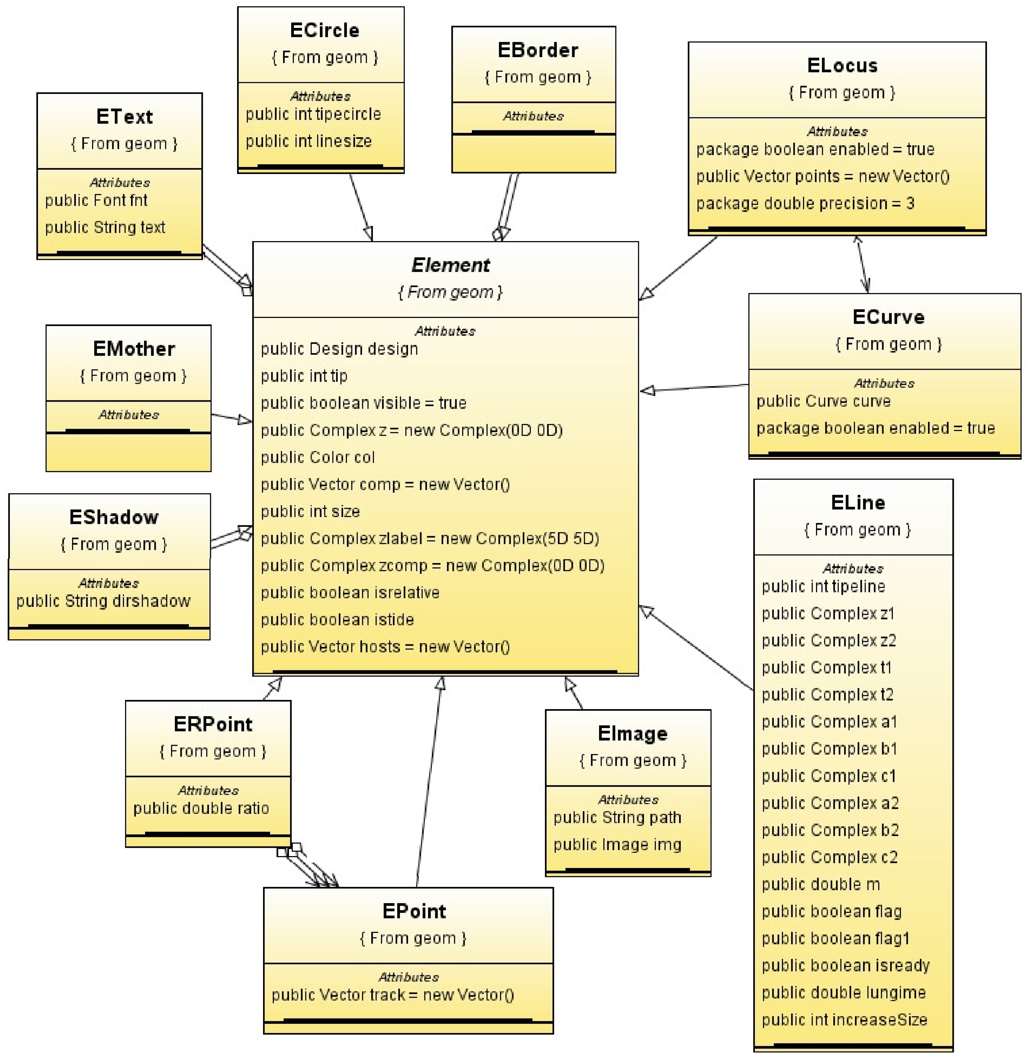
The software system is rather complex; in this section, we discuss some parts of it. If we refer to the dynamic curves presented in the previous section, Figure 7 reveals the links between various classes used in the corresponding module.
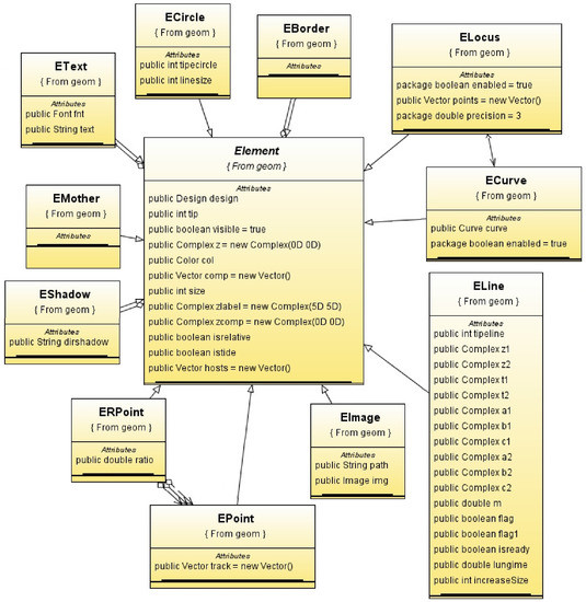
Figure 7.
The software classes for dynamic curves, together with their links.
We can remark that the classes’ modelling geometric entities are built starting from the central class ‘Element’. This approach emphasizes a suitable design, both from a conceptual viewpoint and an implementation viewpoint. Conceptually, each entity has the same abstract model that can derive particular models with specific properties and behaviour. This is visible by the fact that objects as ‘ECircle’, ‘ECurve’ and ‘ELine’ inherit the central entity ‘Element’.
From the implementation point of view, this design fruitfully uses the concepts of the object-oriented programming, such as code reuse through class hierarchies, polymorphism and data encapsulation. It is worth to note that the code for graphical representation is separated from the code describing the main control of the system. This fact is supported by the association relations between the elements providing the graphical representation and those providing the main control of the system; for instance we have a relation ‘eshadow’ between ‘Element’ and ‘EShadow’. To conclude, the design is suitable to modelling and representing dynamic geometric entities.
Complex numbers are used for the representation of the geometric elements. The plane is represented through a system of coordinates xOy, in which the origin O can be easily modified (by a mouse click). A geometric element is implemented by an object of class Element having a complex attribute storing its position; a complex number indicates the coordinates of a point (called affix) on the plane—an affix is identified with the complex number z. An element of type ELine is given by the positions of two of its points; an element of type ECircle is given by its centre and radius, etc. An (object) eline of type ELine implements a line with a rotation point; using any point of it, the rotation can be indicated by a mouse. The points of keep their relative positions during a rotation by using the algorithm below. Let us assume that the rotation centre is given by , and is an arbitrary point on .
- Step 1: The distance is computed between the rotation point and the arbitrary point .
- Step 2: By mouse, modify the points representing the line (these points could be located sometimes outside of the visible display, but they can determine the visible part of the line). If the slope of the line becomes in absolute value greater than 1, we rotate the relative system of coordinate of the line 90 degrees to the right; in this way, the slope remains between 0 and 1. Thus, we avoid the computer representation limitations (when the angle is close to 90 degrees).
- Step 3: According to the new position of the line , the coefficients and a are computed. If the slope is less than 1 (in its absolute value), then set and . Otherwise, and .
- Step 4: The position of the point is computed, where the orthogonal line passing through meets by using .This step is necessary to find the correct position of each point with respect to the rotating centre, .
- Step 5: Use ; ; to compute the next position of each point during the rotation.
Theoretically, the geometrical elements and their geometrical relations are provided by equations in the complex plane. This is not always possible because of the discrete representation of pixels on the computer display. Consequently, we use inequalities instead of equalities. For example, the collinearity of three points , and given by the complex number , and is expressed by . The algorithm of our software verifies the condition , where represents the imaginary part of the complex number z and is a (very small) positive number established by the implementer of the system. As a different example, when considering the points , , , with affixes , , and , a condition for verifying that lines and are orthogonal is , where is the real part of complex number z. Moreover, the condition to verify that , , , are on the same circle is . If z is the affix of a point P (obtained after a click on the display), the condition to verify that point P is on the circle of centre a and radius r is .
By using these approximations inequalities, it is possible to accumulate some errors in the computations involving the positions of the geometric elements. To deal properly with these errors, we use the corresponding equations and change the positions of the visible points accordingly. It is worth noting that some errors cannot be avoided due to the restricted representation of numbers in computers.
To appreciate the features of this software (together with several examples), visit: www.math.uaic.ro/drusu/dynamicGeometry/eng/demo.htm (accessed on 15 November 2022).
5. Kinematics of the Mechanical Systems
To design a mechanical system properly by interconnecting several mechanical components, it would be useful to have a flexible tool allowing the simulation of certain complicated scenarios. Such a tool can describe its time-dependent evolution, and identify how the system responds under different input conditions. A proper tool can be used to improve the design and performance, or to discover specific working conditions in order to reach certain requirements.
We use our intuitive software in the kinematic analysis of linkages and the related problems of the kinematic analysis of (over)constrained linkages. The software verifies and maintains consistency between the components and their interactions (joint constraints). The form and the behaviour of the mechanical system evolve simultaneously during the design process; any change made to the form is propagated automatically to its behaviour (eventually, some inconsistencies can be reported). To simulate the mechanical dynamics of these systems with constraints, the algorithms of the software extract and derive the parameters for each component, and joints are determined automatically. The behaviours of the rigid bodies and joints are derived by using the positions and orientations (expressed relative to the axes of a coordinate system) and the forces acting on each component described by the Newton-Euler equations involving the input parameters and the variables related to velocity, acceleration, mass, (twisting) force and inertia tensor. The constraints are integrated properly to provide a safe motion simulation. The degrees of freedom is automatically detected. The algorithms propagate all the interactions throughout the system, offering a large variety of features.
The design space is located on the left side of the working window. The components are drawn with the mouse (whenever the drawn parameter is on). The used coordinate system is located in the lower left corner of the design space; the designer could change it by using the menu on the top toolbar of the window. The coordinate system and the whole system can be changed by using the zoom option (on the same toolbar).
The kinematic behaviour and analysis is displayed on the right side of the working window. This space is used to observe the movement of the mechanical system based on the elements set by using the left toolbar of the window (selected by double-click). The axes of the coordinate system are automatically determined (taking care of the parameters values indicated by the user). Time is on the X-axis, and on the Y-axis are the parameters indicated by the user. Using a timeline, it is possible to move (by using the mouse) this timeline in order to observe the values of the parameter at any moment of time. This movement of the timeline is an event, and the indicated values are acquired by the software; the corresponding answers from the system is displayed in the upper left corner of this space (L: length, A: angle, AR: relative angle, AV: angular velocity, AA: angular acceleration, etc).
We present some examples of simulating mechanical systems by using our interactive software for dynamic geometry, providing some kinematic diagrams of a few mechanisms.
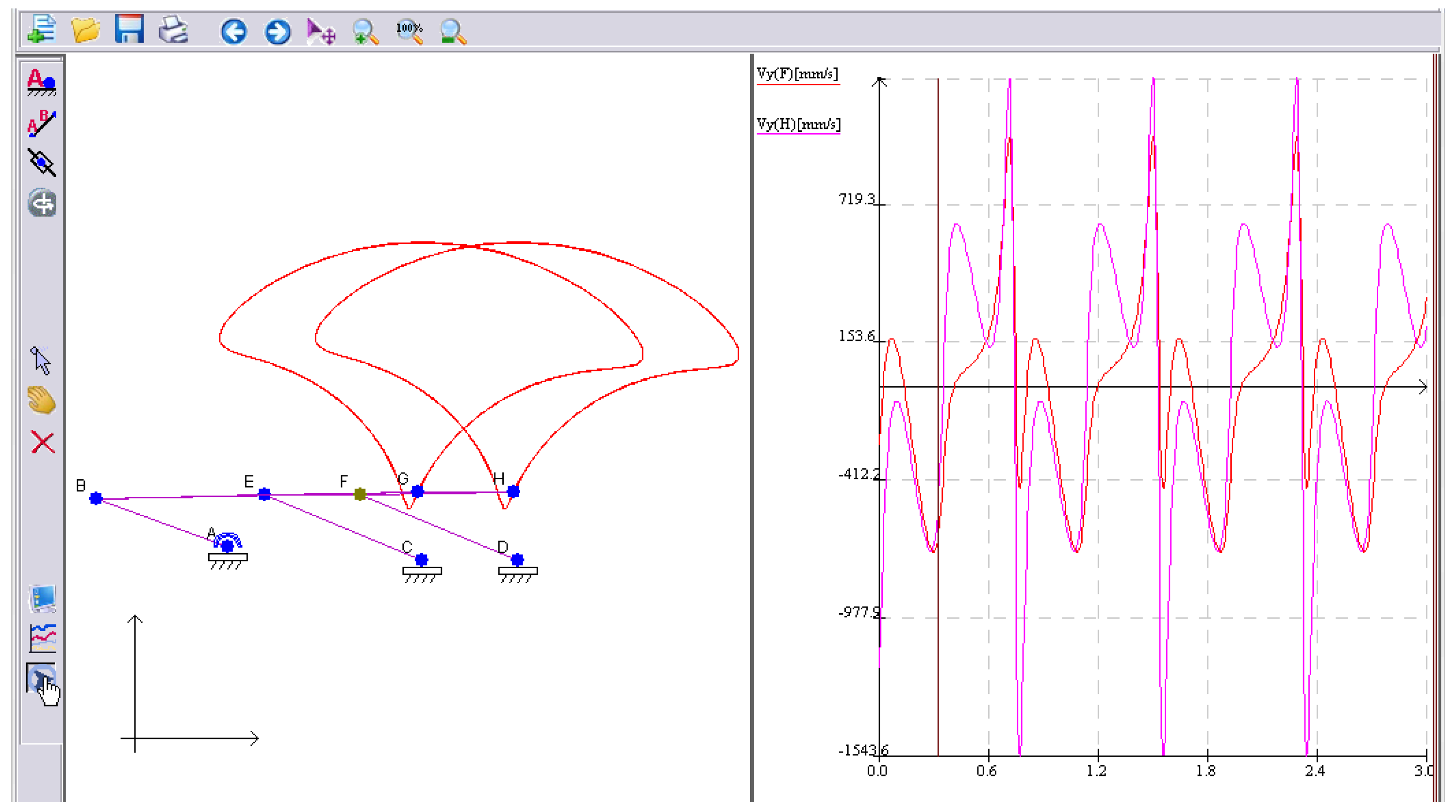
A crankshaft is a mechanism consisting of cranks for which there are attached some connecting rods of an engine. A crankshaft performs a conversion between the motion of a piston into a rotational motion. A connecting rod of a piston engine joins the piston to the crankshaft; in this way, it converts the reciprocating motion of the piston into the rotation motion of the crankshaft. The most common use of the connecting rods is in internal combustion engines.
Let us assume a jointed quadrilateral (a 4-sided polygon) of a crank mechanism working with a combustion engine having a connecting rod. In Figure 8, the trajectory of a point linked to the connecting rod is presented on the left-hand side of the window, where we can observe the mechanism. On the right-hand side, the diagram for the kinematic analysis of the mechanism is presented; the dynamic evolution can help a system designer or system analyst to work properly with this software.
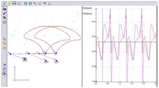
Figure 8.
Kinematic diagram and the trajectory of the connecting rod.
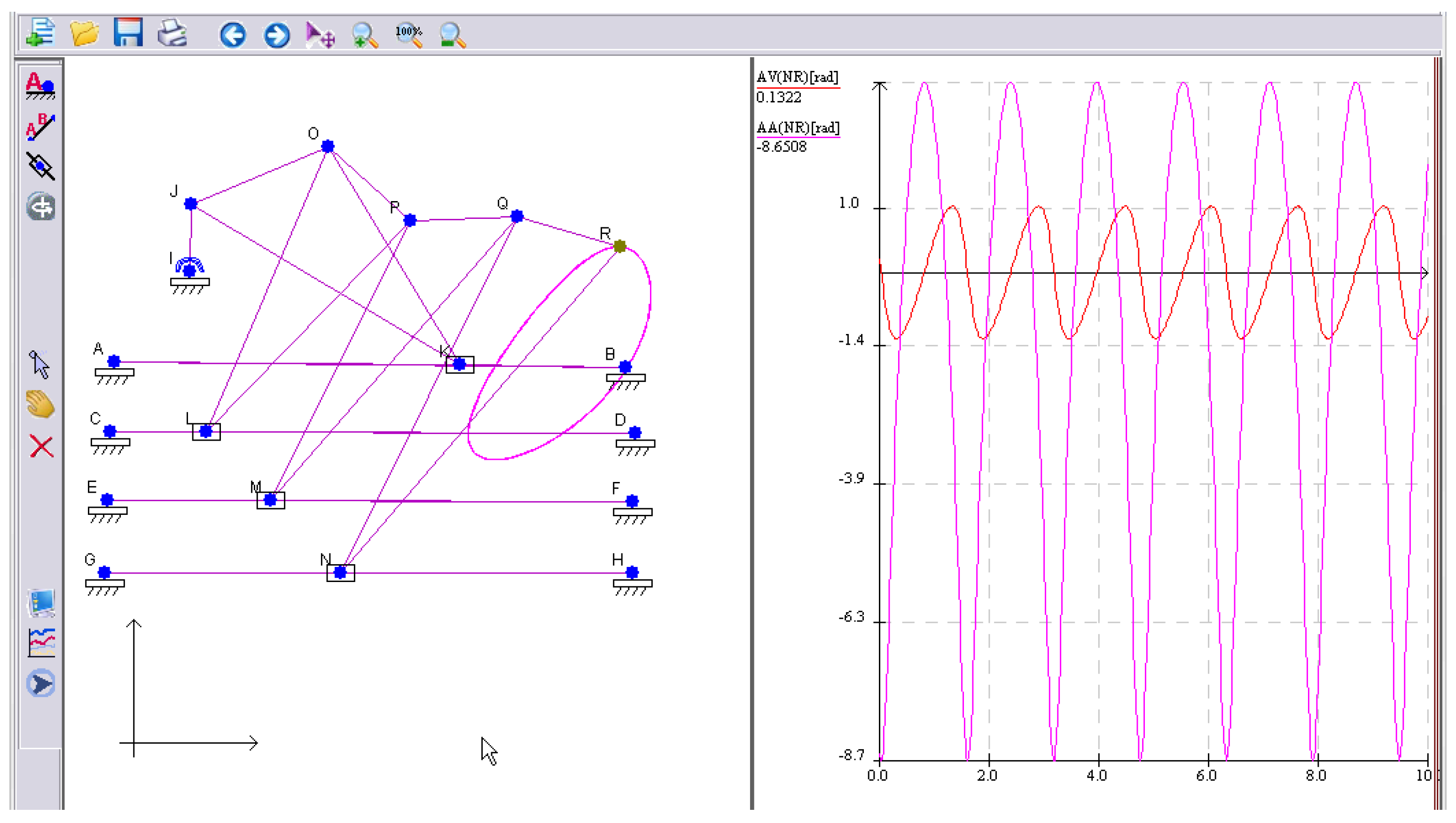
Figure 9 presents a little more complicated mechanism, namely a manipulator-like system used to test a variety of advanced nonlinear control strategies. The articulated manipulator is a robot with rotating joints; these kind of articulated robots can vary from basic two-jointed systems to complex structures with 10 (or even more) interacting joints.
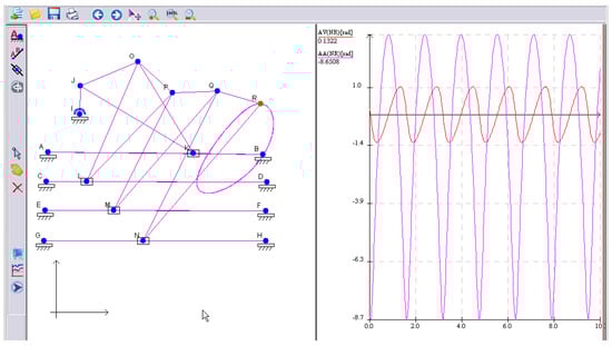
Figure 9.
Simulation of an articulated manipulator, and its kinematic diagram.
The simulation presents the functioning of a mechanism consisting of a series of crank-piston mechanisms connected to the rod of the previous mechanism included in a structural group of four pistons. In robotics, an (end) effector is the part of the robot that interacts with the environment. The trajectory of the effector point is plotted on the right-hand diagram.
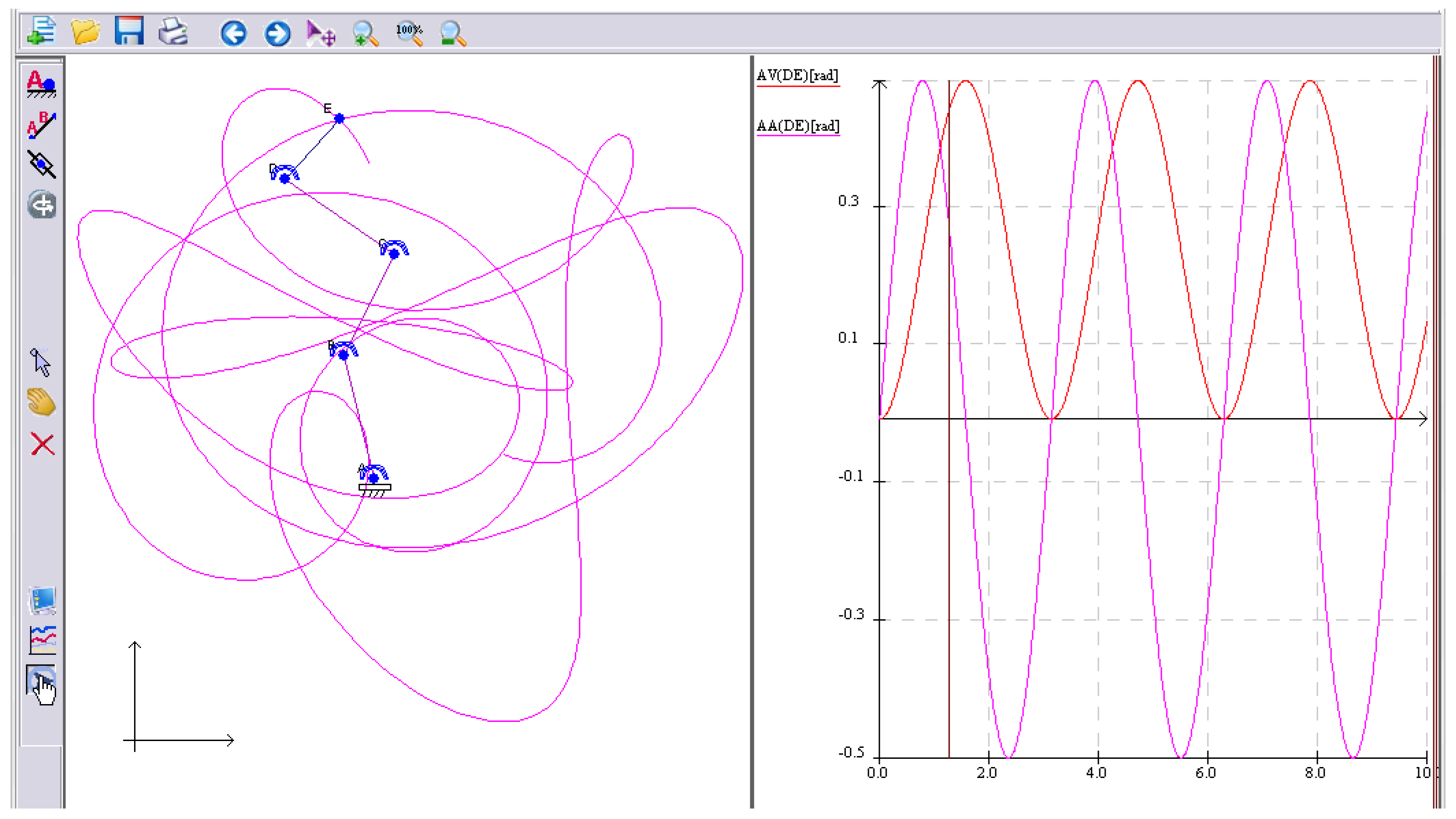
In a different scenario (Figure 10), it is simulated a plane manipulator with four grades of mobility. The four trainers have different laws of motion (depending on time) introduced as mathematical expressions. The simulation of the complex motion is presented on the left-hand side, and the kinematic diagram is presented on the right-hand side of Figure 10.
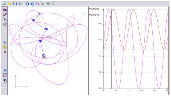
Figure 10.
Simulation of a manipulator with four trainers.
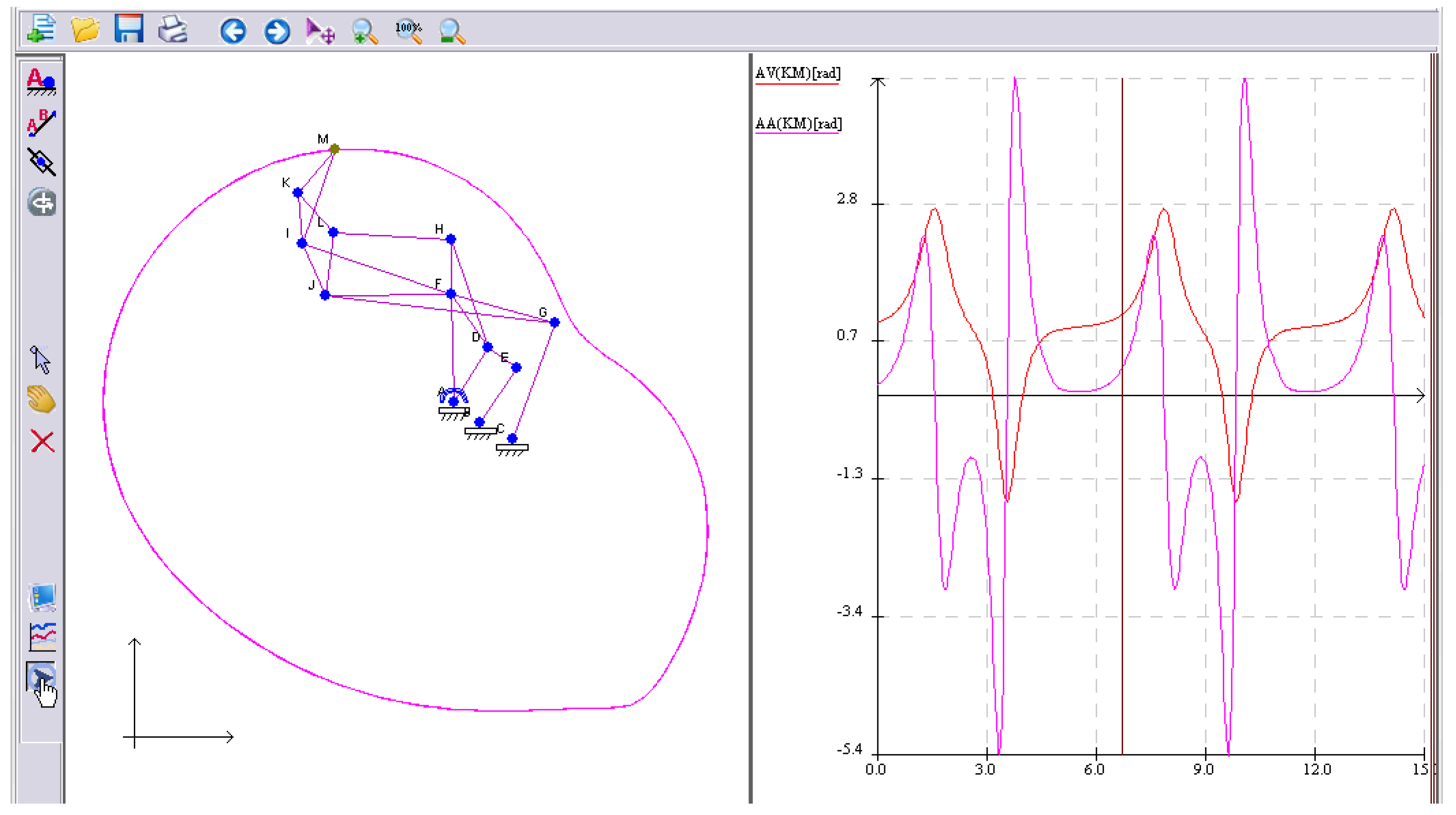
Figure 11 presents the simulation of a mechanism of higher complexity working as a mechanical arm (a system between robots and bio-mechanisms). Its design has only kinematic and rotation elements. The trajectory of the end effector could be complex.
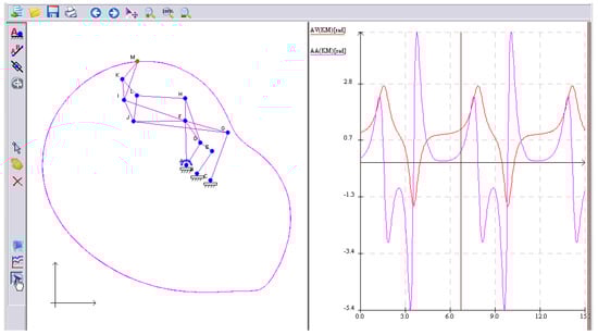
Figure 11.
Simulation of a mechanical arm, together with its kinematic diagram.
These simple examples illustrate in a comprehensible way how our interactive software could be used in the kinematic analysis of linkages. Generally, more complicated mechanisms could be described and analyzed.
6. Conclusions
The mechanical systems interconnecting several components dependant on geometry [2]. This dependence on geometry requires special consideration, especially when employing complicated mechanical and robotic systems [6]. In general, a description of such a mechanical system takes into account the constraints imposed on the motion (expressed as functions of time and of states themselves). The behaviour of various mechanical systems depends on these constraints.
Several methods are used to model mechanical systems of interconnected components based on the application of basic translational and rotational elements; these elements can indeed characterize a great variety of mechanical systems [4]. In this paper, we emphasized on a modern approach (an interactive software) regarding the kinematics of mechanical systems by dynamic geometry. Extending a previous conference paper [5], we present an interactive software for dynamic geometry to be used for designing, simulating and analyzing mechanical systems, and for solving various kinematic and dynamic problems. The software provides various attractive features: a flexible design, simulations involving mobile elements, dynamic homotopy, configurable speeds, use of associated formulas, and working properly with algorithms defined by the user. It is also worth mentioning the parametric curve plots obtained with this software. These aspects improve the design quality, saving time and money (for instance, by detecting inconsistencies and errors early in the design process). These features can be used for several scientific and meaningful tasks. It can be applied in scientific projects for discovering interesting relations in geometry, it can be used to define and simulate systems in several engineering disciplines, and for various interactive experiments. It could be used by scientists, but also by teachers.
There exist several software systems dealing with plane geometry [7]. We mention the interactive geometry software Cinderella [8], a system designed many years ago (see http://www.cinderella.de/tiki-index.php (accessed on 15 November 2022)), but still in use and working well. Recently, GeoGebra became popular [9,10]; GeoGebra merges features of dynamic geometry and computer algebra (visit www.geogebra.org (accessed on 15 November 2022) for details). There also exists large software systems with advanced modules for geometry; among the most complex are Mathematica, Maple and Matlab. In all of them, it is possible to define the equations of a curve; however, none of them provides the possibility of dynamic homotopy and transformations of a curve depending on its parameters.
Regarding the kinematics of mechanical systems, we mention the following software tools. SolidWorks (www.solidworks.com (accessed on 15 November 2022)) is a commercial computer-aided engineering application. The disadvantages of SolidWorks are given by the high cost and the fact that it requires a powerful Windows computer (being limited only to a Windows operating system). Even regarding its 2D functionality, our approach could be a better option. MechAnalyzer (www.roboanalyzer.com/mechanalyzer.html (accessed on 15 November 2022)) is a free software mainly used for teaching 3D mechanisms; it is related to a software used to teach and learn robotics [11]. It can perform a synthesis of four-bar mechanisms. Its dynamic geometry module is less developed. Moreover, it does not present kinematic diagrams, and so the kinematic analysis of linkages and other related issues are not explicitly treated. GIM (www.ehu.eus/compmech/software (accessed on 15 November 2022)) is devoted to the kinematics and dynamics analysis of planar and spatial mechanisms [12]. It is limited by the use of the Windows operating system. Sometimes, its interface is not so intuitive. Comparing with our approach, it also has some dynamic geometry limitations. The kinematics software ASOM (visit asom.eu/en/ (accessed on 15 November 2022) for details) is a licensed software for linkage design and for the simulation of multi-bar mechanisms. It offers an intuitive handling, and several advanced features for synthesis, analysis and optimization of the multi-bar systems. The licensing costs and requirements reduce its benefits.
By comparing our approach with these software tools, we consider that an important advantage is given by the intuitive and simple way of working with it; this is due to the algorithms we use, and the way of describing and manipulating the mechanisms.
Author Contributions
Conceptualization, G.C. and D.R.; methodology, G.C. and D.R.; software, G.C. and D.R.; validation, G.C. and D.R.; formal analysis, G.C. and D.R.; investigation, G.C. and D.R.; resources, G.C. and D.R.; data curation, G.C. and D.R.; writing—original draft preparation, G.C. and D.R.; writing—review and editing, G.C. and D.R.; visualization, G.C. and D.R.; supervision, G.C. and D.R.; project administration, G.C. and D.R.; funding acquisition, G.C. and D.R. All authors have read and agreed to the published version of the manuscript.
Funding
This research received no external funding.
Acknowledgments
Many thanks to the anonymous referees for their useful remarks and comments.
Conflicts of Interest
The authors declare no conflict of interest.
References
- Kleppner, D.; Kolenkow, R. An Introduction to Mechanics; Cambridge University Press: Cambridge, UK, 2013. [Google Scholar]
- Uicker, J.J.; Pennock, G.R.; Shigley, J.E. Theory of Machines and Mechanisms, 5th ed.; Oxford University Press: Oxford, UK, 2016. [Google Scholar]
- Gao, X. Building Dynamic Mathematical Models with Geometry Expert. In Proceedings of the Asian Technology Conference in Mathematics, Guangzhou, China, 17–21 December 1999; pp. 153–162. [Google Scholar]
- Norton, R.L. Kinematics and Dynamics of Machinery; McGraw-Hill: New York, NY, USA, 2013. [Google Scholar]
- Ciobanu, G.; Rusu, D. Pythagoras: An Interactive Environment for Plane Geometry. In Proceedings of the 3rd Conference on Intelligent Computer Communication and Processing, Cluj-Napoca, Romania, 6–8 September 2007; pp. 283–286. [Google Scholar]
- Dresig, H.; Holzweissig, F. Dynamics of Machinery: Theory and Applications; Springer: Berlin/Heidelberg, Germany, 2010. [Google Scholar]
- Wu, W.; Gao, X. Mathematics mechanization and applications after thirty years. Front. Comput. Sci. China 2007, 1, 1–8. [Google Scholar] [CrossRef]
- Richter-Gebert, J.; Kortenkamp, U.H. The Interactive Geometry Software Cinderella; Springer: Berlin/Heidelberg, Germany, 1999. [Google Scholar]
- Hohenwarter, M. GeoGebra: Vom Autodesign zur Computerschriftart. Inform. Spektrum 2009, 32, 18–22. [Google Scholar] [CrossRef]
- Hohenwarter, M.; Kovacs, Z.; Recio, T. Using Automated Reasoning Tools to Explore Geometric Statements and Conjectures. In Proof Technology in Mathematics Research and Teaching; Springer: Berlin/Heidelberg, Germany, 2019; pp. 215–236. [Google Scholar]
- Saha, S.K. Introduction to Robotics; Tata McGraw-Hill: New York, NY, USA, 2014. [Google Scholar]
- Petuya, V.; Macho, E.; Altuzarra, O.; Pinto, C.; Hernandez, A. Educational Software Tools for the Kinematic Analysis of Mechanisms. Comput. Appl. Eng. Educ. 2014, 22, 72–86. [Google Scholar] [CrossRef]
Publisher’s Note: MDPI stays neutral with regard to jurisdictional claims in published maps and institutional affiliations. |
© 2022 by the authors. Licensee MDPI, Basel, Switzerland. This article is an open access article distributed under the terms and conditions of the Creative Commons Attribution (CC BY) license (https://creativecommons.org/licenses/by/4.0/).