Abstract
Deep learning—in particular, deep neural networks (DNNs)—as a mesh-free and self-adapting method has demonstrated its great potential in the field of scientific computation. In this work, inspired by the Deep Ritz method proposed by Weinan E et al. to solve a class of variational problems that generally stem from partial differential equations, we present a coupled deep neural network (CDNN) to solve the fourth-order biharmonic equation by splitting it into two well-posed Poisson’s problems, and then design a hybrid loss function for this method that can make efficiently the optimization of DNN easier and reduce the computer resources. In addition, a new activation function based on Fourier theory is introduced for our CDNN method. This activation function can reduce significantly the approximation error of the DNN. Finally, some numerical experiments are carried out to demonstrate the feasibility and efficiency of the CDNN method for the biharmonic equation in various cases.
MSC:
35J58; 65N35; 68T07
1. Introduction
In this paper, we consider the numerical solution of the biharmonic equation
where is a polygonal or polyhedral domain in Euclidean space (d is the dimension) with a piecewise Lipschitz boundary that satisfies an interior cone condition, is a given function and is a standard Laplace operator. The operators and are expressed as
respectively.
A biharmonic equation is a class of common high-order partial differential equations (PDEs) that stems from the field of physics and applied mathematics, especially in elasticity theory and Stokes flow problems; for instance, scattered data fitting with thin plate splines [1], fluid mechanics [2,3] and linear elasticity [4,5]. In the last few decades, many traditional numerical methods have been proposed for dealing with (1), and they can be classified into two categories: a direct (uncoupled) approach and coupled (splitting, mixed) approach.
In terms of the direct approach, there are the finite difference method (FDM) based on its uncoupled scheme [6,7,8,9], finite volume method (FVM) [10,11,12], finite element method (FEM) based on its variational formulation, such as non-conforming FEM [13,14,15], and conforming FEM [16,17]. The idea of the coupled approach is to introduce auxiliary variables and split the biharmonic equation into two coupled Poisson equations. Based on this coupled scheme, the finite difference technique [9,18,19], finite element technique and mixed element technique [20,21,22,23,24] are naturally used to solve the two second-order equations. In addition, the collocation method [25,26,27] and radial basis functions (RBF) method [28,29,30] are also approaches considered to solve (1).
However, the traditional methods will encounter the curse of an irregular domain and high dimension. Deep learning, especially deep neural networks (DNNs), have expressed a remarkable performance in solving mathematical problems in scientific computations and engineering applications based on its great potential in nonlinear approximation; for example, utilizing DNNs to solve partial differential equations [31,32,33,34], stochastic differential equations [35], inverse problems [36], molecular modeling [37], etc. Specially, the Deep Ritz method (DRM) [32] and physical information neural network (PINN) [36] have gained more and more attention in PDEs, and they have made wonderful grades for solving various PDEs. Within the architectures of DRM and PINN, some DNN-based methods have been proposed to directly deal with this biharmonic Equation (1) [38,39,40,41,42,43]. Since these DNN-based methods need to compute the second-order or fourth-order derivative of the solution in and the second-order derivative of the solution in , they may consume a large amount of time and computer resources when solving (1). In addition, the authors in [44] proposed a deep mixed residual method (MIM) to solve PDEs with high-order derivatives by splitting it into some first-order systems; however, the PDEs solution and its derivatives share nearly the same DNN and boundary conditions, are not consistent with the mechanism of PDEs and adversely affect the performance of MIM.
In this paper, we investigate addressing the high-order elliptic Equation (1) by combining the Deep Ritz method and the coupled scheme of the biharmonic equation, and then establish a coupled deep neural network architecture (CDNN). Motivated by double triangle series and Fourier expansion, a new activation function with sine and cosine are provided for our CDNN model; it will improve the capability of DNN for approximating a complex target because of it being smooth and local. The application of a trigonometric function as an activation function can also be found in [45,46]. The main contributions of this paper are as follows:
- Based on the coupled scheme of the fourth-order biharmonic Equation (1), we constructed a CDNN architecture for dealing with (1) by means of the Deep Ritz method used to solve variational problems; this architecture is composed of two independent DNNs. Compared with the existing DNN methods, the CDNN will reduce effectively the complexity of the algorithm, save the resources of the computer and make the neural networks easier to train. In the meantime, this model performs remarkably well and obtains considerable results.
- According to the property of spectral bias or frequency preference for the DNN, we introduced a Fourier mapping with sine and cosine as the activation function of the first layer for the DNN model; it can mitigate the pathology of the spectral bias of the DNN. In the viewpoint of function approximation, the DNN model with Fourier mapping mimics the Fourier expansion, in which, the first layer with Fourier mapping can be regarded as a series of Fourier basic functions and the output of the DNN is the (nonlinear) combination of those basis functions.
- By introducing some compared DRM models with different activation functions to solve the original form of the biharmonic equation, we show that our CDNN model performs better when solving (1) in various dimensional space.
The paper is structured as follows. In Section 2, we briefly introduce the framework of the deep neural network and the formulation of ResNet. Then, in Section 3, we construct the CDNN architecture to approximate the solution of the biharmonic equation based on its coupled scheme and provide the options of the activation function. In Section 4, some numerical examples are carried out to test the performance of the developed CDNN model. Section 5 discusses the merits and shortcomings of the CDNN, and provides the opportunity to address related works. Finally, some brief conclusions are made in Section 6.
2. Deep Neural Network and ResNet Architecture
In this section, the related concepts and mathematical formulation of the DNN are briefly introduced. At first, a standard neural unit of a DNN with an input and an output is in the form of
where and are called a weight matrix and bias vector, respectively. Here and thereafter, is a non-linear operator, commonly known as the activation function, and “∘” stands for the elementary-wise operation. Generally, the output of (2) will be transformed by a new weight and a new bias, and the new output will be fed into another activation function. Hence, (2) is also called the hidden layer of the DNN. In other word, the DNN is a nested composition of sequential single linear functions and nonlinear activation functions. Mathematically, the DNN with an input datum and an output can be formulated as
where are the weight matrix and bias vector of the l-th hidden layer, respectively, and is the dimension of the output for the DNN. For convenience, we denote the parameter set by here and thereafter.
The residual neural network (ResNet) technique [47] has been widely used in deep neural networks for solving PDEs; it can not onl skilfully overcome the vanishing gradient problem of DNN in backpropagation, but can also well improve the capacity of the DNN to approximate the solution and high-order derivatives of PDEs [32,37]. The architecture of ResNet is depicted in the following Figure 1.
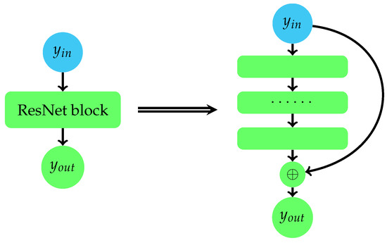
Figure 1.
The architecture of ResNet.
Mathematically, a ResNet block with a one-step connection produces a filtered version for the input , which is as follows:
In this work, we also employed the strategy of a one-step skip connection for two consecutive layers in the DNN if they have the same number of neurons. For those consecutive layers with different neuron numbers, the skip connection step is omitted.
3. Unified coupled DNNs Architecture to Biharmonic Equation
Skilfully decoupling the biharmonic Equation (1) into two Poisson equations, traditional numerical methods such as FEM and FDM obtain a favorable performance with a small number of computing resources and a lower time complexity. By introducing an auxiliary variable , one can rewrite the fourth-order Equation (1) into a couple of second-order equations:
Then, we searched a couple of functions instead of finding a solution for the original problem (1). Generally, the strong solutions of (4) may be non-existent; one can obtain their weak solutions in the given domain . The weak function pair should satisfy and
They are equivalent to the weak version of the Euler–Lagrange equation for the following variational problems:
and
respectively.
The Deep Ritz method based on a deep neural network is an efficient approach for solving variational problems that generally stem from PDEs [32]; it utilizes a parameterized neural network to replace the trial function and changes the original problems into the optimization of neural networks. In addition, some works concerning convergence analysis for DRM are proposed [48,49].
Based on the above results, we then suppose two ansatzes of DNN and as the functions and v, which minimize the variational problem (5) and (6), respectively, where and denote the parameters of underlying DNNs. Substituting into (5) for , we can firstly obtain the following equation:
Since the minimization problem (5) is related to w and is an approximation of w, then we obtain the following equation by replacing v and w with and , respectively, in (6):
Using the Monte Carlo method [50] to calculate the above integration in , we further have
with
and
respectively; here, and thereafter, stands for the samples in with probability density .
Boundary conditions are important constraints for numerical methods such as FDM and FEM to solve PDEs, which ensure the uniqueness and accuracy of the solution for PDEs. Analogously, imposing boundary conditions is also an important issue in DNN representation. Under the boundary constraints of (4), the DNNs and on should satisfy
and
here, and thereafter, stands for the samples on with probability density .
To this end, two individual parameters of DNNs model are optimized by minimizing the following loss function:
with
where and represent the training data of and , respectively. In addition, we introduce a penalty parameter to control the contribution of the boundary for the loss function; it increases gradually as the training process continues.
Our goal is to find two sets of parameters and such that the approximate functions and minimize the functions and . If these loss functions are small enough, then and will be very close to the solution of (4), i.e.,
Remark 1.
In practical implementation, we bundled , and together and trained them by means of a neural network optimizer. These functions in form are related, but they can be trained in parallel.
Remark 2.
By directly transforming the biharmonic Equation (1) into a variational problem, one can easily employ DRM to solve it. The corresponding loss is given by
with
and
where stands for the output of DRM.
In order to obtain the and , one can update the parameters and by means of gradient descent (GD) or stochastic gradient descent (SGD) techniques over the training samples at each iteration. Regarding implementation, SGD is the common optimization method used for deep learning; it only requires the gradient information of a DNN over one or a few samples. In this context, the SGD is given by:
where the “learning rate” decreases with k increasing and . Based on the above discussions, Figure 2 describes the schematic of the CDNN for solving biharmonic Equation (1).
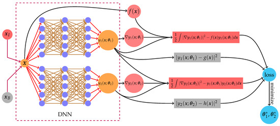
Figure 2.
Schematic of a CDNN for solving the biharmonic equation. The left two DNNs with the same framework(dotted line box) share the input (including and ), and the upper and lower branches output and , which are used to approximate the function w and u, respectively. The right part handles the outputs of DNN and forms the total loss according to PDEs constraints and boundary conditions.
Many experiments have shown that choosing a suitable activation function is crucial for DNNs in various fields. As we have learned, nonlinear activation functions such as , and are the common choice for the DNN model; they will improve the capacity of DNN to deal with various nonlinear problems, such as nonlinear PDEs and classification. Due to the biharmonic equation in this work being a class of high-order PDEs, an activation function with a low-order derivative possibly has an unfavourable effect for DNN when it is used to solve (1). We then consider the activation function with a good regularity, such as tanh. Figure 3 depicts the curves of the tanh function with first-order and second-order derivatives, which shows that the range of derivatives for tanh is small and stable.
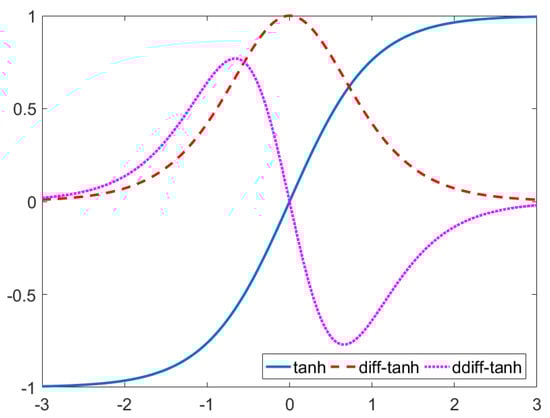
Figure 3.
The curves for tanh function and its derivatives, respectively.
In the viewpoint of function approximation, the first layer with activation functions for the DNN can be regarded as a series of basic functions, and the output of the DNN is the (nonlinear) combination of those basis functions. Recently, the works [51,52] found the phenomenon of spectral bias or frequency preference for DNNs and show that the DNN will firstly capture the low-frequency component, and then some corresponding explanations are made by means of a neural tangent kernel (NTK) [45,53] and Fourier analysis [54,55]. Within this sense of spectral bias and Fourier approximation, a given real function can be expressed by the following sine and cosine expansions:
where are fully connected DNNs or sub-modules of the DNN, respectively, are the frequencies of interest in the target function and will always be included. Obviously, it mimics the Fourier expansion, and the remaining blocks of the DNN (except for the first layer) are used to learn the coefficients of Fourier basis functions.
Choosing a Fourier feature mapping with sine and cosine as the activation function for the DNN model is reasonable; it can mitigate the pathology of spectral bias and enable networks to learn the target function well [45,46]. It is
where is a user-specified vector (it is not trainable) and is consistent with the number of neural units in the first hidden layer for the DNN. By performing the Fourier feature mapping for input points, the input points in may be mapped to ; then, the subsequent modules of the DNN with different activation functions can easily deal with the feature information, such as sigmoid, tanh and ReLU, etc.
4. Numerical Experiments
4.1. Training Setup
In this section, we tested the performance of the CDNN model with the aforementioned activation functions (tanh and Fourier mapping) for solving the biharmonic equation in varying-dimensional spaces. In addition, two types of Deep Ritz methods with tanh and Fourier mapping were introduced to serve as the baseline. These compared methods and their setups are as follows:
- DRM: A normal DNN model with tanh being its activation function for all hidden layers and its output layer being linear.
- FDRM: A normal DNN model with Fourier mapping as the activation function for its first hidden layer, where its activation functions for the remainder hidden layers are chosen as tanh and its output layer is linear. The vector as in (16) is set as , and we will repeat it when the length of is less than the number of neural units for the first hidden layer.
- CDNN: A coupled DNN model with tanh being its activation function for all hidden layers and its output layer being linear.
- FCDNN: A coupled DNN model with Fourier mapping as the activation function for its first hidden layer, where its activation functions for the remainder hidden layers are chosen as tanh and its output layer is linear. The vector as in (16) is set as , and we will repeat it when the length of is less than the number of neural units for the first hidden layer.
We provide the following criteria to evaluate the above models:
where and are the approximate solution of the DNN and exact solution, respectively, for testing points , and represents the number of testing points.
In our numerical experiments, all training and test data were generated with uniform distribution in Euclidean space , and all networks were trained by an Adam optimizer. The initial learning rate was set as with a decay rate of for each training epoch.
For the sake of viewing the training process, we tested our models for every 1000 epochs in the training process and recorded the result at the end. In our codes, the was set as
where the in all our tests, and represents the total number of epoch and was set as 100000 in our all experiments. We performed all neural network training and testing in TensorFlow (version 1.14.0) on a workstation (256-GB RAM, single NVIDIA GeForce GTX 2080Ti 12-GB).
4.2. Numerical Examples
Example 1.
We solved the biharmonic Equation (1) on the unit square domain . The exact solution and force-side are
and
respectively. The boundary conditions on .
In the following tests, we obtained the solution of (1) by means of DRM, FDRM, CDNN and FCDNN, respectively. Their network size is (120, 60, 50, 50, 40), (60, 60, 50, 50, 40), (100, 50, 30, 30, 20) and (50, 50, 30, 30, 20), respectively. It is easy to know that the number of parameters for the methods is 14100, 10800, 14000 and 10000, respectively. At each training epoch, the training dataset was generated from and , which include 3000 interior points and 500 boundary points in , respectively. The testing dataset was uniformly sampled from of mesh-size . We plot the numerical results in Figure 4 and list the final error results in Table 1.
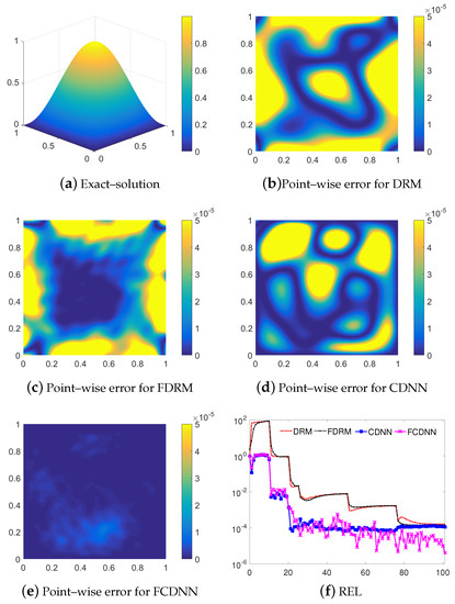
Figure 4.
Testing results for Example 2.

Table 1.
REL and running time of the aforementioned four models for Example 2.
Based on the above results, we can see that the DRM, FDRM, CDNN and FCDNN are all able to approximate the solution of (1), in which, the FCDNN model performs best, and the performances of CDNN, DRM and FDRM are competitive. In terms of the overall errors, the CDNN is stable in all training processes, but the FCDNN is still descending with small oscillations. This means that the Fourier mapping activation function will improve the capability of the CDNN model. Table 1 shows that the CDNNs only cost approximately 0.5 h to solve Equation (1), but the DRMs cost more than 1.05 h. In summary, our CDNN methods not only have a high accuracy, but are also efficient.
Example 2.
We solved the biharmonic Equation (1) on the hexagram domain Ω derived from . The exact solution and force-side are
and
respectively. The functions and on are easy to obtain according to the exact solution; here, we omit it.
In this example, the setups for DRM, FDRM, CDNN and FCDNN are the same as Example 4. At each training epoch, the training dataset was sampled from and , which include 3000 interior points and 500 boundary points, respectively. The testing dataset was randomly sampled from the hexagon domain in . We plot the numerical results in Figure 5 and list the final error results in Table 2.
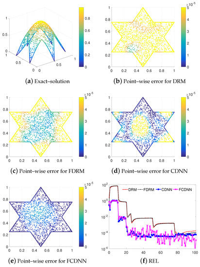
Figure 5.
Testing results for Example 2.
Table 2.
REL and running time of the aforementioned four models for Example 2.
On the irregular domain, the CDNN and FCDNN are still able to obtain the solution of (1), and the performance of FCDNN is superior to that of DRM, FDRM and CDNN. In the meantime, the runtime of CDNNs is also approximately half of DRMs and the performance of FCDNN is still decreasing, with small oscillations when the other three methods become stable.
Example 3.
We solved the biharmonic Equation (1) on a unit cubic domain with some holes. The exact solution is given by
It will naturally induce the boundary conditions and on . By careful calculations, one can obtain the force side; here, we omit it.
When the DRM, FDRM, CDNN and FCDNN are used to solve (1) in the three-dimension space, their network size is set as (200, 100, 80, 80, 60), (100, 100, 80, 80, 60), (100, 80, 60, 60, 40) and (50, 80, 60, 60, 40). The training data set, including 6000 interior points and 1000 boundary points, was randomly sampled from and . A testing dataset was given that includes 1600 random points distributed in . The testing results are plotted in Figure 6 and the final error results are listed in Table 3. For showing these results visually, we projected the point-wise error for the DRM, FDRM, CDNN and FCDNN evaluated on 1600 sample points into a rectangular region with mesh size , respectively. Note that the mapping is only for the purpose of visualization and is independent of the actual coordinates of those points.
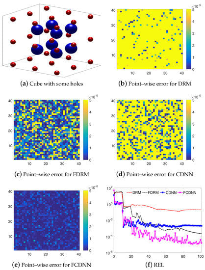
Figure 6.
Testing results for Example 3.
Table 3.
REL and running time of the aforementioned four models for Example 3.
Based on the above results, we can see that the FCDNN still outperforms other models when solving the biharmonic problem (1) in a three-dimensional space, and that the performance of the CDNN becomes a bit weaker than the FDRM. In addition, the point-wise square error of the four models in Figure 6b,c, as well as the overall errors in Figure 6f, show that the performance of FCDNN is much better than that of the other three models. Compared with the case of 2D, the data in Table 3 show the run-time of CDNNs is almost kept unchanged, but the DRMs will cost more time.
Example 4.
We solved the biharmonic Equation (1) on the unit higher-dimensional domain . The exact solution and force-side are
and
respectively. The boundaries of this problem satisfy .
Since the DRM and FDRM needed a large amount of computing resources for this example, our station could not satisfy their requirements; as a result, we only employed the CDNN and FCDNN to solve the biharmonic Equation (1) in eight-dimensional space, where the sizes for the CDNN and FCDNN were set as (300, 200, 200, 100, 100) and (150, 200, 200, 100, 100), respectively. The training data set included 20000 interior points and 5000 boundary points randomly sampled from and . A testing dataset was given that included 1600 random points distributed in . The testing results are plotted in Figure 7 and the final error results are listed in Table 4. Additionally, the point-wise error for CDNN and FCDNN evaluated on 1600 sample points was projected into a rectangular region with mesh size , respectively.
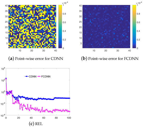
Figure 7.
Testing results for Example 4.
Table 4.
REL and running time of the CDNN and FCDNN for Example 4.
The results in Figure 7 show that the FCDNN still maintains its good performance to approximate the exact solution of (1) in eight-dimensional space; however, the CDNN model will become slightly degenerated. In addition, the relative error of the FCDNN is much smaller than that of the CDNN based on Table 4.
5. Discussion
Compared with the DRM algorithms, the proposed CDNN method can solve the fourth-order biharmonic equation well based on its coupled scheme. It not only effectively reduces the complexity of the DNN algorithm, but also save the resources of the computer. In the meantime, a novel activation function composed of sine and cosine is introduced; it will obviously improve the performance of DNNs in solving a complex target. In a lower dimensional space, the CDNN method costs the least time, and attains the best accuracy. Regarding a high dimensional space, the CDNN can still keep its favorable performance; however, the DRM method cannot work because of the tremendous computational burden. In addition, the idea of a coupled scheme can be extended to the PINN method; then, a coupled PINN method may be developed to solve the PDEs without a variational form or other high-order problems. In this paper, we considered the biharmonic equation with a Neumann boundary; it is suitable for our CDNN method. Thus, more complex boundary conditions, such as the Dirichlet boundary and Robin boundary or other mixed boundaries, may be considered. Different from the case of Neumann, the other boundaries will not naturally induce the boundaries for two networks; thus, it is necessary to carefully design the coupled framework and boundary constraints of the DNN. Further, the performance of the CDNN will be degenerated or even not convergent if all of the networks lack the appropriate boundary conditions. Finally, the first-order optimization methods of the DNN and the sampling technique of training points may have an unfavorable effect on the accuracy and efficiency of DNN; this is an important issue to be solved.
6. Conclusions
By means of a coupled scheme of the biharmonic equation, we proposed a coupled DNN framework to solve this high-order problem in the work. As a class of a meshless method, the CDNN method does not rely on the initial guess and can approximate the solution of the biharmonic equation with a low complexity well. Additionally, a mixed loss function was designed that will enhance the stability and robustness for our model. Furthermore, a novel activation function based on Fourier approximation was introduced for the input layer, and the subsequent hidden layers were chosen as a good regularity function, such as tanh; this strategy can improve the accuracy and convergence rate for the CDNN method. Computational results show that the proposed method is feasible and efficient in solving the (1) in a complex domain and various dimension space. In the future, work is in progress to extend the neural network models to solve other high-order partial differential equations.
Author Contributions
Conceptualization, Methodology and Writing–original draft: X.L.; Methodology and Writing–review & editing: J.W.; Methodology, Supervision and Funding acquisition: L.Z.; Resources, Validation and Project administration: X.T. All authors have read and agreed to the published version of the manuscript.
Funding
This research was funded by National Natural Science Foundation of China(NSFC) OF FUNDER grant number 1871339 and 1186113100.
Data Availability Statement
Not applicable.
Acknowledgments
L.Z. is partially supported by the National Natural Science Foundation of China (NSFC 11871339, 11861131004). This work is also partially supported by HPC of School of Mathematical Sciences at Shanghai Jiao Tong University.
Conflicts of Interest
All authors declare that they have no known competing financial interests or personal relationships that could have appeared to influence the work reported in this paper.
References
- Wahba, G. Spline Models for Observational Data; Society for Industrial and Applied Mathematics: Philadelphia, PA, USA, 1990. [Google Scholar]
- Greengard, L.; Kropinski, M.C. An integral equation approach to the incompressible navier–stokes equations in two dimensions. SIAM J. Sci. Comput. 1998, 20, 318–336. [Google Scholar] [CrossRef]
- Ferziger, J.H.; Peric, M. Computational Methods for Fluid Dynamics; Springer: Berlin/Heidelberg, Germany, 2002. [Google Scholar]
- Christiansen, S. Integral equations without a unique solution can be made useful for solving some plane harmonic problems. IMA J. Appl. Math. 1975, 16, 143–159. [Google Scholar] [CrossRef]
- Constanda, C. The boundary integral equation method in plane elasticity. Proc. Am. Math. Soc. 1995, 123, 3385–3396. [Google Scholar] [CrossRef]
- Gupta, M.M.; Manohar, R.P. Direct solution of the biharmonic equation using noncoupled approach. J. Comput. Phys. 1979, 33, 236–248. [Google Scholar] [CrossRef]
- Altas, I.; Dym, J.; Gupta, M.M.; Manohar, R.P. Multigrid solution of automatically generated high-order discretizations for the biharmonic equation. SIAM J. Sci. Comput. 1998, 19, 1575–1585. [Google Scholar] [CrossRef]
- Ben-Artzi, M.; Croisille, J.P.; Fishelov, D. A fast direct solver for the biharmonic problem in a rectangular grid. SIAM J. Sci. Comput. 2008, 31, 303–333. [Google Scholar] [CrossRef]
- Bialecki, B. A fourth order finite difference method for the Dirichlet biharmonic problem. Numer. Algorithms 2012, 61, 351–375. [Google Scholar]
- Bi, C.J.; Li, L.K. Mortar finite volume method with Adini element for biharmonic problem. J. Comput. Math. 2004, 22, 475–488. [Google Scholar]
- Wang, T. A mixed finite volume element method based on rectangular mesh for biharmonic equations. J. Comput. Appl. Math. 2004, 172, 117–130. [Google Scholar] [CrossRef]
- Eymard, R.; Gallouët, T.; Herbin, R.; Linke, A. Finite volume schemes for the biharmonic problem on general meshes. Math. Comput. 2012, 81, 2019–2048. [Google Scholar] [CrossRef]
- Baker, G.A. Finite element methods for elliptic equations using nonconforming elements. Math. Comput. 1977, 31, 45–59. [Google Scholar] [CrossRef]
- Lascaux, P.; Lesaint, P. Some nonconforming finite elements for the plate bending problem. Rev. Française D’automatique Inform. Rech. Opérationnelle Anal. Numérique 1975, 9, 9–53. [Google Scholar] [CrossRef]
- Morley, L.S.D. The triangular equilibrium element in the solution of plate bending problems. Aeronaut. Q. 1968, 19, 149–169. [Google Scholar] [CrossRef]
- Zienkiewicz, O.C.; Taylor, R.L.; Nithiarasu, P. The Finite Element Method for Fluid Dynamics, 6th ed.; Elsevier Butterworth-Heinemann: Oxford, UK, 2005. [Google Scholar]
- Ciarlet, P. The Finite Element Method for Elliptic Problems; North-Holland Publishing Company: Amsterdam, The Netherlands, 1978. [Google Scholar]
- Smith, J. The coupled equation approach to the numerical solution of the biharmonic equation by finite differences. II. SIAM J. Numer. Anal. 1968, 5, 104–111. [Google Scholar] [CrossRef]
- Ehrlich, L.W. Solving the biharmonic equation as coupled finite difference equations. SIAM J. Numer. Anal. 1971, 8, 278–287. [Google Scholar] [CrossRef]
- Brezzi, F.; Fortin, M. Mixed and Hybrid Finite Element Methods; Springer: New York, NY, USA, 1991. [Google Scholar]
- Cheng, X.L.; Han, W.; Huang, H.C. Some mixed finite element methods for biharmonic equation. J. Comput. Appl. Math. 2000, 126, 91–109. [Google Scholar] [CrossRef]
- Davini, C.; Pitacco, I. An unconstrained mixed method for the biharmonic problem. SIAM J. Numer. Anal. 2000, 38, 820–836. [Google Scholar] [CrossRef]
- Lamichhane, B.P. A stabilized mixed finite element method for the biharmonic equation based on biorthogonal systems. J. Comput. Appl. Math. 2011, 235, 5188–5197. [Google Scholar] [CrossRef]
- Stein, O.; Grinspun, E.; Jacobson, A.; Wardetzky, M. A mixed finite element method with piecewise linear elements for the biharmonic equation on surfaces. arXiv 2019, arXiv:1911.08029. [Google Scholar]
- Mai-Duy, N.; See, H.; Tran-Cong, T. A spectral collocation technique based on integrated Chebyshev polynomials for biharmonic problems in irregular domains. Appl. Math. Model. 2009, 33, 284–299. [Google Scholar] [CrossRef]
- Bialecki, B.; Karageorghis, A. Spectral Chebyshev collocation for the Poisson and biharmonic equations. SIAM J. Sci. Comput. 2010, 32, 2995–3019. [Google Scholar] [CrossRef]
- Bialecki, B.; Fairweather, G.; Karageorghis, A.; Maack, J. A quadratic spline collocation method for the Dirichlet biharmonic problem. Numer. Algorithms 2020, 83, 165–199. [Google Scholar] [CrossRef]
- Mai-Duy, N.; Tanner, R. An effective high order interpolation scheme in BIEM for biharmonic boundary value problems. Eng. Anal. Bound. Elem. 2005, 29, 210–223. [Google Scholar] [CrossRef]
- Adibi, H.; Es’haghi, J. Numerical solution for biharmonic equation using multilevel radial basis functions and domain decomposition methods. Appl. Math. Comput. 2007, 186, 246–255. [Google Scholar] [CrossRef]
- Li, X.; Zhu, J.; Zhang, S. A meshless method based on boundary integral equations and radial basis functions for biharmonic-type problems. Appl. Math. Model. 2011, 35, 737–751. [Google Scholar] [CrossRef]
- E, W.; Han, J.; Jentzen, A. Deep learning-based numerical methods for high-dimensional parabolic partial differential equations and backward stochastic differential equations. Commun. Math. Stat. 2017, 5, 349–380. [Google Scholar] [CrossRef]
- Weinan, E.; Yu, B. The deep ritz method: A deep learning-based numerical algorithm for solving variational problems. Commun. Math. Stat. 2018, 1, 1–12. [Google Scholar]
- Berg, J.; Nyström, K. A unified deep artificial neural network approach to partial differential equations in complex geometries. Neurocomputing 2018, 317, 28–41. [Google Scholar] [CrossRef]
- Sirignano, J.; Spiliopoulos, K. DGM: A deep learning algorithm for solving partial differential equations. J. Comput. Phys. 2018, 375, 1339–1364. [Google Scholar] [CrossRef]
- Nabian, M.A.; Meidani, H. A deep learning solution approach for high-dimensional random differential equations. Probabilistic Eng. Mech. 2019, 57, 14–25. [Google Scholar] [CrossRef]
- Raissi, M.; Perdikaris, P.; Karniadakis, G.E. Physics-informed neural networks: A deep learning framework for solving forward and inverse problems involving nonlinear partial differential equations. J. Comput. Phys. 2019, 378, 686–707. [Google Scholar] [CrossRef]
- Zou, Z.; Zhang, H.; Guan, Y.; Zhang, J. Deep residual neural networks resolve quartet molecular phylogenies. Mol. Biol. Evol. 2020, 37, 1495–1507. [Google Scholar] [CrossRef] [PubMed]
- Guo, H.; Zhuang, X.; Rabczuk, T. A deep collocation method for the bending analysis of Kirchhoff plate. CMC-Comput. Mater. Contin. 2019, 59, 433–456. [Google Scholar] [CrossRef]
- Samaniego, E.; Anitescu, C.; Goswami, S.; Nguyen-Thanh, V.M.; Guo, H.; Hamdia, K.; Zhuang, X.; Rabczuk, T. An energy approach to the solution of partial differential equations in computational mechanics via machine learning: Concepts, implementation and applications. Comput. Methods Appl. Mech. Eng. 2020, 362, 112790. [Google Scholar] [CrossRef]
- Li, W.; Bazant, M.Z.; Zhu, J. A physics-guided neural network framework for elastic plates: Comparison of governing equations-based and energy-based approaches. Comput. Methods Appl. Mech. Eng. 2021, 383, 113933. [Google Scholar] [CrossRef]
- Mohammad, V.; Ehsan, H.; Maryam, K.; Nasser, K. A physics-informed neural network approach to solution and identification of biharmonic equations of elasticity. J. Eng. Mech. 2021, 148, 04021154. [Google Scholar]
- Zhongmin, H.; Zhen, X.; Yishen, Z.; Linxin, P. Deflection-bending moment coupling neural network method for the bending problem of thin plates with in-plane stiffness gradient. Chin. J. Theor. Appl. Mech. 2021, 53, 25–41. [Google Scholar]
- Goswami, S.; Anitescu, C.; Rabczuk, T. Adaptive fourth-order phase field analysis using deep energy minimization. Theor. Appl. Fract. Mech. 2020, 107, 102527. [Google Scholar] [CrossRef]
- Lyu, L.; Zhang, Z.; Chen, M.; Chen, J. MIM: A deep mixed residual method for solving high-order partial differential equations. J. Comput. Phys. 2022, 452, 110930. [Google Scholar] [CrossRef]
- Wang, S.; Wang, H.; Perdikaris, P. On the eigenvector bias of Fourier feature networks: From regression to solving multi-scale PDEs with physics-informed neural networks. Comput. Methods Appl. Mech. Eng. 2021, 384, 113938. [Google Scholar] [CrossRef]
- Tancik, M.; Srinivasan, P.; Mildenhall, B.; Fridovich-Keil, S.; Raghavan, N.; Singhal, U.; Ramamoorthi, R.; Barron, J.; Ng, R. Fourier features let networks learn high frequency functions in low dimensional domains. Adv. Neural Inf. Process. Syst. 2020, 33, 7537–7547. [Google Scholar]
- He, K.; Zhang, X.; Ren, S.; Sun, J. Deep residual learning for image recognition. In Proceedings of the IEEE Conference on Computer Vision and Pattern Recognition, Las Vegas, NE, USA, 27–30 June 2016; pp. 770–778. [Google Scholar]
- Duan, C.; Jiao, Y.; Lai, Y.; Li, D.; Yang, Z. Convergence rate analysis for deep ritz method. Commun. Comput. Phys. 2022, 31, 1020–1048. [Google Scholar] [CrossRef]
- Jiao, Y.; Lai, Y.; Lo, Y.; Wang, Y.; Yang, Y. Error analysis of deep Ritz methods for elliptic equations. arXiv 2021, arXiv:2107.14478. [Google Scholar]
- Robert, C.P.; Casella, G. Monte Carlo Statistical Methods; Springer: New York, NY, USA, 2004. [Google Scholar]
- Xu, Z.Q.J.; Zhang, Y.; Luo, T.; Xiao, Y.; Ma, Z. Frequency principle: Fourier analysis sheds light on deep neural networks. Commun. Comput. Phys. 2020, 28, 1746–1767. [Google Scholar] [CrossRef]
- Rahaman, N.; Baratin, A.; Arpit, D.; Draxler, F.; Lin, M.; Hamprecht, F.; Bengio, Y.; Courville, A. On the spectral bias of neural networks. In Proceedings of the International Conference on Machine Learning, Long Beach, CA, USA, 9–15 June 2019; pp. 5301–5310. [Google Scholar]
- Jacot, A.; Gabriel, F.; Hongler, C. Neural tangent kernel: Convergence and generalization in neural networks. Adv. Neural Inf. Process. Syst. 2018, 8571–8580. [Google Scholar]
- Xu, Z.J. Understanding training and generalization in deep learning by fourier analysis. arXiv 2018, arXiv:1808.04295. [Google Scholar]
- Xu, Z.Q.J.; Zhang, Y.; Xiao, Y. Training behavior of deep neural network in frequency domain. In Proceedings of the International Conference on Neural Information Processing, Vancouver, BC, Canada, 8–14 December 2019; Springer: Berlin/Heidelberg, Germany, 2019; pp. 264–274. [Google Scholar]


Publisher’s Note: MDPI stays neutral with regard to jurisdictional claims in published maps and institutional affiliations. |
© 2022 by the authors. Licensee MDPI, Basel, Switzerland. This article is an open access article distributed under the terms and conditions of the Creative Commons Attribution (CC BY) license (https://creativecommons.org/licenses/by/4.0/).