
Global Stability of a Reaction–Diffusion Malaria/COVID-19 Coinfection Dynamics Model


Abstract
1. Introduction
2. Reaction–Diffusion Malaria/COVID-19 Model with Immune Response
3. Properties of Solutions
- (1)
- The uninfected equilibrium always exists;
- (2)
- The SARS-CoV-2-free equilibrium without immune response exists if ;
- (3)
- The SARS-CoV-2-free equilibrium exists if ;
- (4)
- The malaria-free equilibrium without immune response exists if ;
- (5)
- The malaria-free equilibrium exists if ;
- (6)
- The malaria/COVID-19 coinfection immune-free equilibrium exists if and ;
- (7)
- The malaria/COVID-19 coinfection equilibrium exists if , , and .
- (1)
- The uninfected equilibrium , whereThus, the equilibrium always exists.
- (2)
- The malaria single-infection without immunity equilibrium is given by , , wherewhere . We note that and are positive, while and are positive for . Thus, exists when . Here, is a threshold parameter, which specifies the establishment of malaria infection.
- (3)
- The malaria single-infection with immunity equilibrium . The components are given bywhere . We see that , , and are always positive, while when . Therefore, exists if . is a threshold parameter which sets the initiation of antibody immune response against malaria merozoites.
- (4)
- The SARS-CoV-2 single-infection without immunity equilibrium is defined as . The components are given bywhere . Notably, and are always positive, while and are positive when . Here, is a threshold parameter which determines the establishment of SARS-CoV-2 infection.
- (5)
- The SARS-CoV-2 single-infection with immunity is given by , , wherewhere . We see that , , and are always positive, while if . Hence, exists if . The threshold parameter marks the establishment of antibody immunity against SARS-CoV-2 infection.
- (6)
- The malaria/SARS-CoV-2 coinfection without immunity equilibrium is given by , , whereThe components and are always positive. and are positive when , while and are positive when . Consequently, exists when and .
- (7)
- The malaria/SARS-CoV-2 coinfection with immunity equilibrium is given by , , whereBy substituting in the fourth equation of model (1), we obtainThus, fulfills the following equationLet us define a function as follows:whereBy computing the value of at , we obtainwhere . We note that ifIn addition, we find thatThus, if
4. Global Stability of Equilibria
5. Numerical Simulations
- (1)
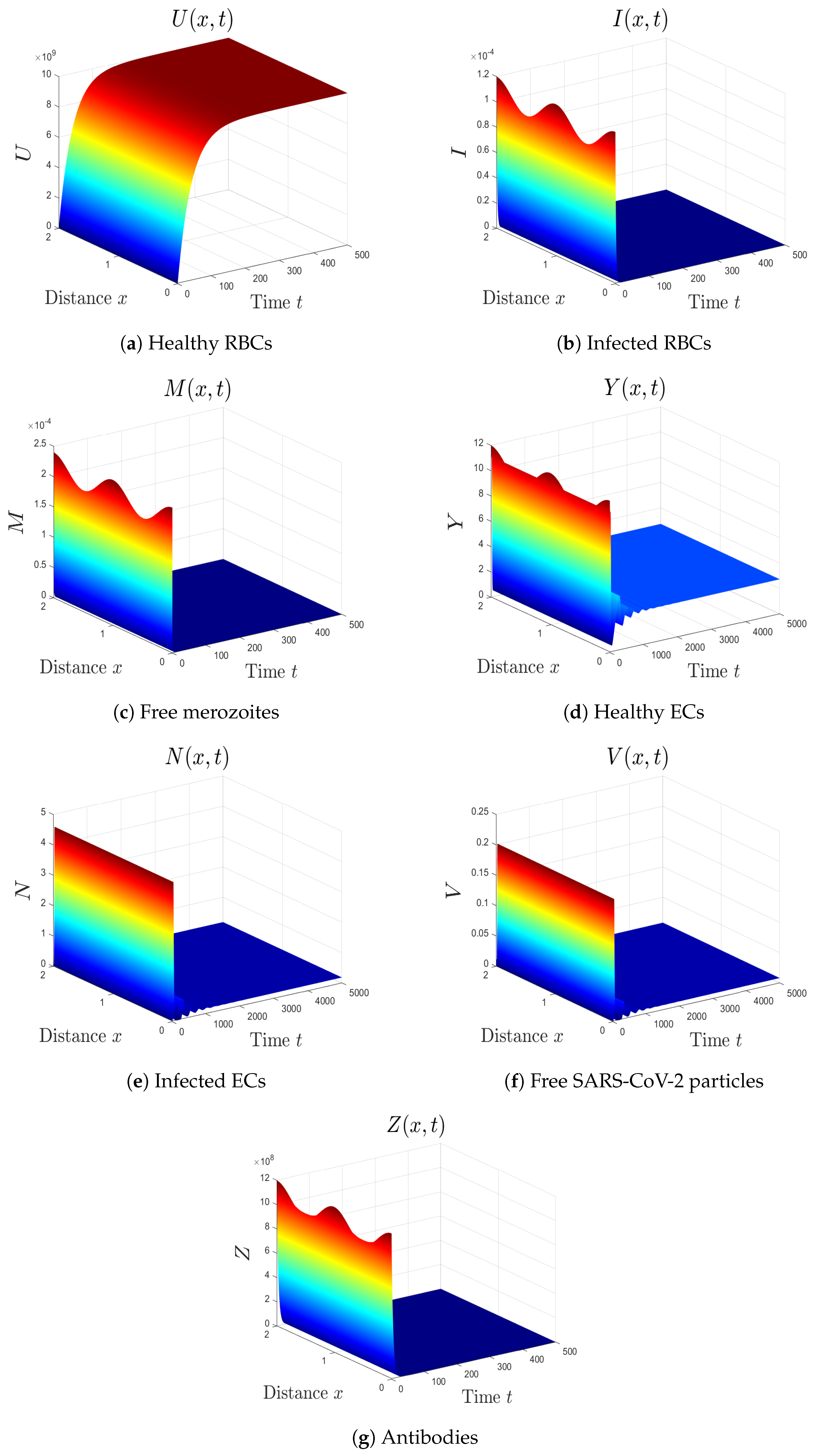
- The varied parameters are . This yields and . This implies that the equilibrium is GAS (see Figure 1), which agrees with Theorem 2. This simulates an individual who has recovered from both malaria and SARS-CoV-2 infections.
- (2)
- The selected parameters are . Then, we obtain , , and . Figure 2 shows that the numerical results agree with the analytical results of Theorem 4. The equilibrium is GAS. This case describes a patient who only has malaria with inactive antibody immune response.
- (3)
- The varied parameters are . This yields and . From Figure 3, we see that the equilibrium is GAS, which illustrates Theorem 4. This case represents a patient who has only malaria with an active antibody immune response.
- (4)
- By choosing , we obtain , , and . Figure 4 illustrates the global asymptotic stability of the equilibrium as given by Theorem 5. The patient in this situation suffers from SARS-CoV-2 single-infection with inactive immunity.
- (5)
- By selecting we obtain , . Accordingly, the equilibrium is GAS (see Figure 5). This result comes in agreement with Theorem 6. The patient in this situation has SARS-CoV-2 single-infection with active immunity. The activation of the antibody immunity causes a reduction in the number of SARS-CoV-2 particles.
- (6)
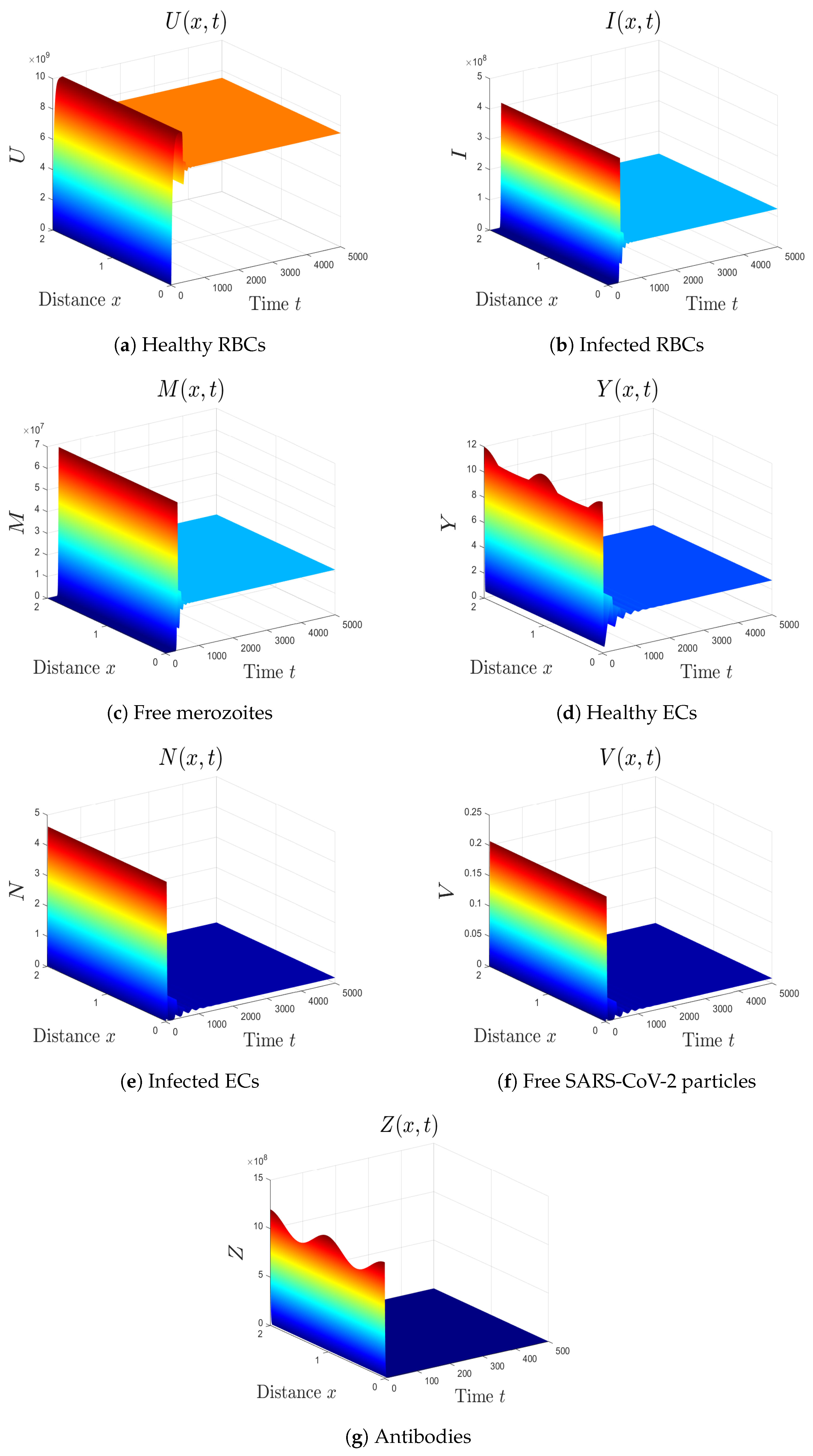
- We take . This gives , , and . Thus, the equilibrium is GAS (see Figure 6), which agrees with Theorem 7. Here, the coinfection of malaria and COVID-19 occurs but with inactive antibody immunity. The inactivation of immunity enhances the replication of both SARS-CoV-2 particles and malaria merozoites, which worsens the health state of the patient.
- (7)
- We select . In this case, the threshold parameters are given as , , and . In line with Theorem 8, the equilibrium is GAS (see Figure 7). Under these circumstances, the coinfection of malaria and COVID-19 occurs with active antibody immunity. This action works on reducing the concentrations of both malaria merozoites and SARS-CoV-2 particles.
5.1. Sensitivity Analysis
5.1.1. Sensitivity Analysis of
5.1.2. Sensitivity Analysis of
6. Results and Discussion
- (1)
- The uninfected equilibrium always exists. Moreover, is GAS if and . This situation represents an individual who recovered from both malaria and SARS-CoV-2 infections.
- (2)
- The malaria single-infection without immunity equilibrium exists if . In addition, is GAS if and . This simulates the situation of malaria mono-infection patient with inactive immunity.
- (3)
- The malaria single-infection with immunity equilibrium exists if . Moreover, is GAS if . At this point, the antibody immune response is activated to eradicate malaria merozoites.
- (4)
- The SARS-CoV-2 single-infection without immunity equilibrium exists if . In addition, is GAS if and . This point simulates the situation of a patient who is only infected by SARS-CoV-2 and the immune response is inactive.
- (5)
- The SARS-CoV-2 single-infection with immunity equilibrium exists if . It is GAS when . The immune response is activated in the SARS-CoV-2 mono-infection patient.
- (6)
- The malaria/COVID-19 coinfection without immunity equilibrium exists if and . It is GAS when . Here, the coinfection occurs with inactive immune response.
- (7)
- The malaria/COVID-19 coinfection with immunity equilibrium exists, and it is GAS if , , and . This point represents the occurrence of malaria/COVID-19 coinfection with an active antibody immune response.
6.1. Conclusions
6.2. Future Works
Supplementary Materials
Author Contributions
Funding
Data Availability Statement
Acknowledgments
Conflicts of Interest
References
- Wilairatana, P.; Masangkay, F.; Kotepui, K.; Milanez, G.; Kotepui, M. Prevalence and characteristics of malaria among COVID-19 individuals: A systematic review, meta-analysis, and analysis of case reports. PLoS Neglected Trop. Dis. 2021, 15, e0009766. [Google Scholar] [CrossRef]
- Akula, S.M.; Abrams, S.L.; Steelman, L.S.; Candido, S.; Libra, M.; Lerpiriyapong, K.; Cocco, L.; Ramazzotti, G.; Ratti, S.; Follo, M.Y.; et al. Cancer therapy and treatments during COVID-19 era. Adv. Biol. Regul. 2020, 77, 100739. [Google Scholar] [CrossRef]
- Jyotsana, N.; King, M. The impact of COVID-19 on cancer risk and treatment. Cell. Mol. Bioeng. 2020, 2016, 5230219. [Google Scholar] [CrossRef]
- Hussein, M.; Albashir, A.; Elawad, O.; Homeida, A. Malaria and COVID-19: Unmasking their ties. Malar. J. 2020, 19, 457. [Google Scholar] [CrossRef]
- Di Gennaro, F.; Marotta, C.; Locantore, P.; Pizzol, D.; Putoto, G. Malaria and COVID-19: Common and different findings. Trop. Med. Infect. Dis. 2020, 5, 141. [Google Scholar] [CrossRef]
- Coronavirus Disease (COVID-19), Vaccine Tracker, World Health Organization (WHO). 2021. Available online: https://covid19.trackvaccines.org/agency/who/ (accessed on 1 October 2022).
- The U.S. Food and Drug Administration. Know Your Treatment Options for COVID-19. 2021. Available online: https://www.fda.gov/consumers/consumer-updates/know-your-treatment-options-covid-19 (accessed on 1 October 2022).
- Elaiw, A.M.; Al Agha, A.D. Global analysis of a reaction–diffusion within-host malaria infection model with adaptive immune response. Mathematics 2020, 8, 563. [Google Scholar] [CrossRef]
- Malaria, Fact Sheets, World Health Organization (WHO). 2021. Available online: https://www.who.int/news-room/fact-sheets/detail/malaria (accessed on 1 October 2022).
- Sebastiao, C.; Gaston, C.; Paixao, J.; Sacomboio, E.; Neto, Z.; de Vasconcelos, J.N.; Morais, J. Coinfection between SARS-CoV-2 and vector-borne diseases in Luanda, Angola. J. Med. Virol. 2021, 94, 366–371. [Google Scholar] [CrossRef]
- Pusparani, A.; Henrina, J.; Cahyadi, A. Co-infection of COVID-19 and recurrent malaria. J. Infect. Dev. Ctries. 2021, 15, 625–629. [Google Scholar] [CrossRef]
- Chanda-Kapata, P.; Kapata, N.; Zumla, A. COVID-19 and malaria: A symptom screening challenge for malaria endemic countries. Int. J. Infect. Dis. 2020, 94, 151–153. [Google Scholar] [CrossRef]
- Indari, O.; Baral, B.; Muduli, K.; Mohanty, A.; Swain, N.; Mohakud, N.K.; Jha, H.C. Insights into Plasmodium and SARS-CoV-2 co-infection driven neurological manifestations. Biosaf. Health 2021, 3, 230–234. [Google Scholar] [CrossRef]
- Mahajan, N.N.; Kesarwani, S.N.; Shinde, S.S.; Nayak, A.; Modi, D.N.; Mahale, S.D.; Gajbhiye, R.K. Co-infection of malaria and dengue in pregnant women with SARS-CoV-2. Int. J. Gynecol. Obstet. 2020, 151, 459–462. [Google Scholar] [CrossRef]
- Hussein, R.; Guedes, M.; Ibraheim, N.; Ali, M.M.; El-Tahir, A.; Allam, N.; Abuakar, H.; Pecoits-Filho, R.; Kotanko, P. Co-infection of malaria and early clearance of SARS-CoV-2 in healthcare workers. J. Med. Virol. 2021, 93, 2431–2438. [Google Scholar]
- Hussein, R.; Guedes, M.; Ibraheim, N.; Ali, M.M.; El-Tahir, A.; Allam, N.; Abuakar, H.; Pecoits-Filho, R.; Kotanko, P. Impact of COVID-19 and malaria coinfection on clinical outcomes: A retrospective cohort study. Clin. Microbiol. Infect. 2022, 28, 1152.e1–1152.e6. [Google Scholar] [CrossRef]
- Kalungi, A.; Kinyanda, E.; Akena, D.; Kaleebu, P.; Bisangwa, I. Less Severe Cases of COVID-19 in Sub-Saharan Africa: Could Co-infection or a Recent History of Plasmodium falciparum Infection Be Protective? Front. Immunol. 2021, 12, 565625. [Google Scholar] [CrossRef]
- Parodi, A.; Cozzani, E. Coronavirus disease 2019 (COVID 19) and Malaria. Med. Hypotheses 2020, 143, 110036. [Google Scholar] [CrossRef]
- Iesa, M.; Osman, M.; Hassan, M.; Dirar, A.; Abuzeid, N.; Mancuso, J.J.; Pandey, R.; Mohammed, A.A.; Borad, M.J.; Babiker, H.M. SARS-CoV-2 and Plasmodium falciparum common immunodominant regions may explain low COVID-19 incidence in the malaria-endemic belt. New Microbes New Infect. 2020, 38, 100817. [Google Scholar] [CrossRef]
- Anderson, R.; May, R.; Gupta, S. Nonlinear phenomena in host-parasite interactions. Parasitology 1989, 99, S59–S79. [Google Scholar] [CrossRef]
- Hetzel, C.; Anderson, R. The within-host cellular dynamics of bloodstage malaria: Theoretical and experimental studies. Parasitology 1996, 113, 25–38. [Google Scholar] [CrossRef]
- Saul, A. Models for the in-host dynamics of malaria revisited: Errors in some basic models lead to large over-estimates of growth rates. Parasitology 1998, 117, 405–407. [Google Scholar] [CrossRef]
- Hoshen, M.; Heinrich, R.; Stein, W.; Ginsburg, H. Mathematical modelling of the within-host dynamics of Plasmodium falciparum. Parasitology 2000, 121, 227–235. [Google Scholar] [CrossRef]
- Iggidr, A.; Kamgang, J.; Sallet, G.; Tewa, J. Global analysis of new malaria intrahost models with a competitive exclusion principle. SIAM J. Appl. Math. 2006, 67, 260–278. [Google Scholar] [CrossRef]
- Tumwiine, J.; Mugisha, J.; Luboobi, L. On global stability of the intra-host dynamics of malaria and the immune system. J. Math. Anal. Appl. 2008, 341, 855–869. [Google Scholar] [CrossRef]
- Orwa, T.; Mbogo, R.; Luboobi, L. Mathematical model for the in-host malaria dynamics subject to malaria vaccines. Lett. Biomath. 2018, 5, 222–251. [Google Scholar] [CrossRef]
- Asamoah, J.; Jin, Z.; Sun, G.; Seidu, B. Sensitivity assessment and optimal economic evaluation of a new COVID-19 compartmental epidemic model with control interventions. Chaos Soiltons Fractals 2021, 146, 110885. [Google Scholar] [CrossRef]
- Currie, C.; Fowler, J.; Kotiadis, K.; Monks, T. How simulation modelling can help reduce the impact of COVID-19. J. Simul. 2020, 14, 83–97. [Google Scholar] [CrossRef]
- Krishna, M.V.; Prakash, J. Mathematical modelling on phase based transmissibility of Coronavirus. Infect. Dis. Model. 2020, 5, 375–385. [Google Scholar] [CrossRef]
- Rajagopal, K.; Hasanzadeh, N.; Parastesh, F.; Hamarash, I.; Jafari, S.; Hussain, I. A fractional-order model for the novel coronavirus (COVID-19) outbreak. Nonlinear Dyn. 2020, 101, 711–718. [Google Scholar] [CrossRef]
- Chen, T.; Rui, J.; Wang, Q.; Zhao, Z.; Cui, J.A.; Yin, L. A mathematical model for simulating the phase-based transmissibility of a novel coronavirus. Infect. Dis. Poverty 2020, 9, 24. [Google Scholar] [CrossRef]
- Liu, Z.; Magal, P.; Seydi, O.; Webb, G. Understanding unreported cases in the 2019-nCoV epidemic outbreak in Wuhan, China, and the importance of major public health interventions. SSRN Electronic J. 2020, 1–12. [Google Scholar] [CrossRef]
- Du, S.Q.; Yuan, W. Mathematical modeling of interaction between innate and adaptive immune responses in COVID-19 and implications for viral pathogenesis. J. Med. Virol. 2020, 92, 1615–1628. [Google Scholar] [CrossRef]
- Li, C.; Xu, J.; Liu, J.; Zhou, Y. The within-host viral kinetics of SARS-CoV-2. Math. Biosci. Eng. 2020, 17, 2853–2861. [Google Scholar] [CrossRef]
- Ghosh, I. Within host dynamics of SARS-CoV-2 in humans: Modeling immune responses and antiviral treatments. arXiv 2020, arXiv:2006.02936. [Google Scholar] [CrossRef]
- Pinky, L.; Dobrovolny, H.M. SARS-CoV-2 coinfections: Could influenza and the common cold be beneficial? J. Med. Virol. 2020, 92, 2623–2630. [Google Scholar] [CrossRef]
- Elaiw, A.M.; Al Agha, A.D.; Azoz, S.A.; Ramadan, E. Global analysis of within-host SARS-CoV-2/HIV coinfection model with latency. Eur. Phys. J. Plus 2022, 137, 1–22. [Google Scholar] [CrossRef]
- Elaiw, A.M.; Al Agha, A.D. Global dynamics of SARS-CoV-2/cancer model with immune responses. Appl. Math. Comput. 2021, 408, 126364. [Google Scholar] [CrossRef]
- Al Agha, A.D.; Elaiw, A.M. Global dynamics of SARS-CoV-2/malaria model with antibody immune response. Math. Eng. 2022, 19, 8380–8410. [Google Scholar] [CrossRef]
- Takoutsing, E.; Temgoua, A.; Yemele, D.; Bowong, S. Dynamics of an intra-host model of malaria with periodic antimalarial treatment. Int. J. Nonlinear Sci. 2019, 27, 148–164. [Google Scholar]
- Elaiw, A.M.; Al Agha, A.D.; Alshaikh, M.A. Global stability of a within-host SARS-CoV-2/cancer model with immunity and diffusion. Int. J. Biomath. 2022, 15, 2150093. [Google Scholar] [CrossRef]
- Zhang, Y.; Xu, Z. Dynamics of a diffusive HBV model with delayed Beddington-DeAngelis response. Nonlinear Anal. Real World Appl. 2014, 15, 118–139. [Google Scholar] [CrossRef]
- Xu, Z.; Xu, Y. Stability of a CD4+ T cell viral infection model with diffusion. Int. J. Biomath. 2018, 11, 1850071. [Google Scholar] [CrossRef]
- Smith, H.L. Monotone Dynamical Systems: An Introduction to the Theory of Competitive and Cooperative Systems; American Mathematical Society: Providence, RI, USA, 1995. [Google Scholar]
- Protter, M.H.; Weinberger, H.F. Maximum Principles in Differential Equations; Prentic Hall: Englewood Cliffs, NJ, USA, 1967. [Google Scholar]
- Henry, D. Geometric Theory of Semilinear Parabolic Equations; Springer: New York, NY, USA, 1993. [Google Scholar]
- Khalil, H.K. Nonlinear Systems; Prentice-Hall: Englewood Cliffs, NJ, USA, 1996. [Google Scholar]
- Elaiw, A.; Al Agha, A. Global dynamics of reaction–diffusion oncolytic M1 virotherapy with immune response. Appl. Math. Comput. 2020, 367, 124758. [Google Scholar] [CrossRef]
- Almocera, A.S.; Quiroz, G.; Hernandez-Vargas, E.A. Stability analysis in COVID-19 within-host model with immune response. Commun. Nonlinear Sci. Numer. Simul. 2020, 95, 105584. [Google Scholar] [CrossRef]
- Bellomo, N.; Burini, D.; Outada, N. Multiscale models of Covid-19 with mutations and variants. Netw. Heterog. Media 2022, 17, 293–310. [Google Scholar] [CrossRef]
- Bellomo, N.; Burini, D.; Outada, N. Pandemics of mutating virus and society: A multi-scale active particles approach. Philos. Trans. A Math. Phys. Eng. Sci. 2022, 380, 20210161. [Google Scholar] [CrossRef]


| Parameter | Definition | Value | Reference |
|---|---|---|---|
| Production rate of healthy RBCs | [21] | ||
| Recruitment rate of healthy ECs | 0.02241 | [33] | |
| Incidence rate constant of RBCs | Varied | – | |
| Incidence rate constant of ECs | Varied | – | |
| Number of merozoites produced from an infected RBC | 16 | [20] | |
| Removal rate constant of merozoites by antibodies | [21] | ||
| Removal rate constant of SARS-CoV-2 particles by antibodies | [49] | ||
| e | Generation rate constant of SARS-CoV-2 by infected ECs | 0.24 | [33] |
| Proliferation rate constant of antibodies by merozoites | Varied | – | |
| Proliferation rate constant of antibodies by SARS-CoV-2 | Varied | – | |
| Death rate constant of healthy RBCs | 0.025 | [21] | |
| Death rate constant of infected RBCs | 0.5 | [26] | |
| Death rate constant of merozoites | 48 | [21] | |
| Death rate constant of healthy ECs | [33] | ||
| Death rate constant of infected ECs | [33] | ||
| Death rate constant of SARS-CoV-2 particles | 5.36 | [33] | |
| Death rate constant of antibodies | Varied | – | |
| Diffusion coefficient of healthy RBCs | 0.1 | Assumed | |
| Diffusion coefficient of infected RBCs | 0.1 | Assumed | |
| Diffusion coefficient of merozoites | 0.2 | Assumed | |
| Diffusion coefficient of healthy ECs | 0.01 | Assumed | |
| Diffusion coefficient of infected ECs | 0.01 | Assumed | |
| Diffusion coefficient of SARS-CoV-2 particles | 0.2 | Assumed | |
| Diffusion coefficient of antibodies | 0.2 | Assumed |
| Parameter | Sensitivity Index |
|---|---|
| 1 | |
| 1 | |
| 1 | |
| Parameter | Sensitivity Index |
|---|---|
| e | 1 |
| 1 | |
| 1 | |
Publisher’s Note: MDPI stays neutral with regard to jurisdictional claims in published maps and institutional affiliations. |
© 2022 by the authors. Licensee MDPI, Basel, Switzerland. This article is an open access article distributed under the terms and conditions of the Creative Commons Attribution (CC BY) license (https://creativecommons.org/licenses/by/4.0/).
Share and Cite
Elaiw, A.M.; Al Agha, A.D. Global Stability of a Reaction–Diffusion Malaria/COVID-19 Coinfection Dynamics Model. Mathematics 2022, 10, 4390. https://doi.org/10.3390/math10224390
Elaiw AM, Al Agha AD. Global Stability of a Reaction–Diffusion Malaria/COVID-19 Coinfection Dynamics Model. Mathematics. 2022; 10(22):4390. https://doi.org/10.3390/math10224390
Chicago/Turabian StyleElaiw, Ahmed M., and Afnan D. Al Agha. 2022. "Global Stability of a Reaction–Diffusion Malaria/COVID-19 Coinfection Dynamics Model" Mathematics 10, no. 22: 4390. https://doi.org/10.3390/math10224390
APA StyleElaiw, A. M., & Al Agha, A. D. (2022). Global Stability of a Reaction–Diffusion Malaria/COVID-19 Coinfection Dynamics Model. Mathematics, 10(22), 4390. https://doi.org/10.3390/math10224390