Article

SCAFG: Classifying Single Cell Types Based on an Adaptive Threshold Fusion Graph Convolution Network

1
School of Mathematics and Physics, Wuhan Institute of Technology, Wuhan 430205, China
2
School of Science, East China Jiaotong University, Nanchang 330013, China
*
Author to whom correspondence should be addressed.
Mathematics 2022, 10(18), 3407; https://doi.org/10.3390/math10183407
Submission received: 6 August 2022 / Revised: 31 August 2022 / Accepted: 15 September 2022 / Published: 19 September 2022

Abstract

:
Single-cell RNA sequencing (scRNA-seq) technology has been a significant direction for single-cell research due to its high accuracy and specificity, as it enables unbiased high-throughput studies with minimal sample sizes. The continuous improvement of scRNA-seq technology has promoted parallel research on single-cell multi-omics. Instead of sequencing bulk cells, analyzing single cells inspires greater discovery power for detecting novel genes without prior knowledge of sequence information and with greater sensitivity when quantifying rare variants and transcripts. However, current analyses of scRNA-seq data are usually carried out with unsupervised methods, which cannot take advantage of the prior distribution and structural features of the data. To solve this problem, we propose the SCAFG (Classifying Single Cell Types Based on an Adaptive Threshold Fusion Graph Convolution Network), a semi-supervised single-cell classification model that adaptively fuses cell-to-cell correlation matrices under various thresholds according to the distribution of cells. We tested the performance of the SCAFG in identifying cell types on diverse real scRNA-seq data; then, we compared the SCAFG with other commonly used semi-supervised algorithms, and it was shown that the SCAFG can classify single-cell data with a higher accuracy.

1. Introduction

The study of gene expression matrices is a critical step in single-cell RNA sequencing analysis [1,2,3]. We can further study the correlations between cells by analyzing a gene expression matrix and creating a molecular map of a cell’s developmental lineage, thus promoting the analysis of the genome, transcriptome, epigenome, and proteome of a single cell. In most cases, we do not know most of the cell types, and it takes much effort to discover them. Even if we know the cell types, it is possible for people to accidentally mislabel the cells with multiple labels. So, we need a mechanical, automated algorithm that recognizes cell types using only a subset of cells. Therefore, the effective application of semi-supervised learning algorithms and obtention of satisfying classification results by using as few single-cell types as possible are fields worth investigating [4,5].
At present, the common semi-supervised learning algorithms mainly include semi-supervised support vector machines (S3VMs) [6], generative semi-supervised models [7], self-training [8], collaborative training (co-training) [9], and graph-theory-based methods [10,11]. The core of supervised support vector machine classification is the use of structural risk minimization [12], while the semi-supervised form of an SVM, S3VM, aims to find a decision boundary in the low-density interval of unlabeled data [13]. Similarly to the principle of entropy regularization, S3VMs make full use of the distribution of unlabeled data and keep unlabeled data as far as possible from the decision boundary; S3VMs indicate that the decision boundary goes as far as possible through low-density regions of unlabeled data, but not through dense unlabeled data. If this assumption is not satisfied, S3VMs may lead to poor performance. Supervised support vector machines use structural risk minimization for classification  [12], while semi-supervised support vector machines also use the spatial distribution information of unlabeled data [14]. The choice of a decision hyperplane should concentrate on the consistent distribution of low-density unlabeled and labeled data [13]. However, if this assumption is not true, information about the spatial distribution of unlabeled data can mislead the decision hyperplane and lead to worse performance than that obtained when using only labeled data. Generative semi-supervised learning is a method based on a generative model. Generative semi-supervised learning methods assume that all data are generated by the same underlying model, whether they are labeled or not. This assumption makes it possible to link unlabeled samples to learning objectives through the parameters of the latent model [15]. The labels of unlabeled samples can be regarded as the missing parameters of the model, which can usually be solved by a maximum likelihood estimation based on the expectation maximization (EM) algorithm. However, the model assumption must be accurate, that is, the assumed generative model must be consistent with the real data distribution; otherwise, using unlabeled data will reduce the generalization performance. Self-training splits the labeled data into a training set and a test set. Firstly, a classification algorithm is trained on the labeled training data. A trained classifier is used to predict the class labels of all unlabeled data, and among these predicted class labels, the one with the highest accuracy is considered to be a pseudo-label [16]. The pseudo-labeled data are concatenated with the correctly labeled training data. Secondly, the classifier is retrained on the combined pseudo-labeled and correctly labeled training data. A trained classifier is used to predict the class label of the labeled test data. Finally, the above steps are repeated until either the predicted class label no longer satisfies a specific probability threshold or no more unlabeled data remain. Co-training is a divergence-based method that assumes that each datum can be classified from different angles and that different classifiers can be trained from different angles; then, these classifiers that are trained from different angles are used to classify unlabeled samples, and the unlabeled samples that are believed to be credible are selected and added to the training set. Since these classifiers are trained from different angles, they can form a complementarity and improve the classification accuracy.
Semi-supervised algorithms have made great progress in the last twenty years because of the rise of artificial neural networks [17,18,19]. The label propagation algorithm is a graph-based semi-supervised learning method [20]. The basic idea is to predict the label information of unlabeled nodes from the label information of the labeled nodes and use the relationships between samples to build a complete graph model. The label of each node is propagated to adjacent nodes according to the similarity. At each step of the node propagation, each node updates its label according to the label of the adjacent node. The greater the similarity with the node is, the greater the influence weight of the neighboring nodes on its labeling will be. The more consistent the labels of similar nodes are, the easier it is for the labels to be propagated. In the process of propagation, the label of the labeled data is kept unchanged so that it passes the label to the unlabeled data. Finally, when the iteration ends, the probability distributions of similar nodes tend to be similar and can be classified into one class [21]. In fact, there are many genes in each cell. This means that every single cell has a high dimension of features, which cannot be learned by using a single classical classifier. Therefore, we consider using a GCN (graph convolutional neural network) to process high-dimensional complicated connections [22,23,24]. A GCN transforms the similarities between cells into the connections between graph edges and further extracts the classification features of edges through a convolution operation. On account of its powerful feature extraction capabilities, it has shown good capabilities in semi-supervised scRNA-seq. However, many parameters need to be adjusted in the practical application of this algorithm; the key to solving the problem is the conversion of the gene expression matrix in the cell into a graph that effectively reflects the similarity relationships between cells. In previous work, Peng proposed the SCMAG [25], which divides the similarity matrices of cells through four different thresholds and then aggregates the obtained matrices for semi-supervised classification with a GCN. However, there is a problem: It cannot select the optimal number of aggregations or the optimal threshold for aggregation according to the data distribution in different single-cell datasets.
To address this problem, we propose the SCAFG, which adaptively fuses cell association matrices under different thresholds according to the cell data distribution, allowing the GCN to fully exploit its performance. Figure 1 depicts the workflow of the SCAFG. Then, we tested the algorithm on different datasets, proving that the SCAFG has the best classification capability among the semi-supervised algorithms.

2. Materials and Methods

2.1. Real Datasets

In this paper, we collected five public single-cell datasets to test the performance of the SCAFG. Each column in the dataset denotes an observation or cell, while each row denotes a feature or gene. These datasets’ raw files are listed in Table 1, and all were downloaded from the Gene Expression Omnibus (GEO) with the GEO accession number.

2.2. Data Normalization

The dimension of the gene expression matrix X is O ( N × G ) , which means that each column has N cells and each row has G genes. Because the count starts from zero, in reality, X ( i , j ) represents the expression level of the ( j + 1 ) t h gene in the ( i + 1 ) t h cell. The expression levels in the gene expression matrix vary widely and have numerous zero values, so we employed PsiNorm to normalize the single-cell data [31]:
X ˜ ( i , : ) = X ( i , : ) × α ^ i = X ( i , : ) × G j = 1 G log x i j + 1
Here, α ^ i is used as a multiplicative normalization factor, X ( i , : ) is equal to the vector of counts of cell i, and  X ˜ ( i , : ) is the normalized vector of X ( i , : ) .

2.3. Cosine Similarity

After data normalization, we obtained the normalized matrix X ˜ ( N , G ) ; next, we transformed the cell-to-gene relationships into cell-to-cell relationships, so we adopted cosine similarity to measure the similarity between cells and map the element values to ( 0 , 1 ) [32]:
M ( i , j ) = X ˜ ( i , : ) · X ˜ ( j , : ) X ˜ ( i , : ) × X ˜ ( j , : )
where X ˜ ( i , : ) denotes the i t h row of X ˜ ( N , G ) , and “·” denotes the inner product. X ˜ ( i , : ) denotes the L 2 -norm of X ˜ ( i , : ) , and M ( i , j ) is the similar value in the i t h row and j t h column.

2.4. Threshold Segmentation

We used different thresholds to divide the similarity matrix M into different incidence matrices:
T = T k = 0.1 × k : k = 1 , 2 , 3 , · · · , 9
S = S n : n = 1 , 2 , 3 , · · · , 9
S k i j = 1 , M ( i , j ) T k 0 , M ( i , j ) < T k
where T k are thresholds, S k denotes the incidence matrix after the segmentation of threshold T k , the dimension of S k is N × N , and N is the number of cells. S k i j denotes the value in the i t h row and j t h column, where 1 indicates two cells are relevant and 0 indicates that two cells are irrelevant.

2.5. Similarity Distance Between Matrices

From Equation ( 5 ) , we obtained 9 individual incidence matrices; each incidence matrix represented the relationships of the connections between cells under the threshold. We considered that the similarity between different incidence matrices could be measured by a value, so we decided to construct a matrix H to depict the similarity distance between incidence matrices. The dimension of H was 9 × 9 , and these values were stored in H. For instance, for the incidence matrix S i and incidence matrix S j , their similarity can be defined as the same number of all corresponding elements in the incidence matrix. Therefore, H ( i , j ) indicates the similarity distance between incidence matrices S i and S j ; a greater value of H ( i , j ) denotes that S i and S j are more similar. The structure is shown in Algorithm 1.
Algorithm 1 Construction of the Similarity Distance Matrix H
Require: Incidence matrix: S = S n , n = 1 , 2 , 3 , . . . , 9 ;
  For each S n in S, they have the same dimension O ( S n 0 , S n 1 ) , S n 0 = S n 1 ;
Ensure:
  1: for x = 0 ; x < 8 ; x + + do
  2:  for  y = x + 1 ; y < 9 ; y + + do
  3:    N = 0 ;
  4:   Calculate  H ( x , y ) :
  5:   for  i = 0 ; i < S x 0 1 ; i + + do
  6:    for  j = i + 1 ; j < S x 1 ; j + +  do
  7:     if  S x i j = = S y i j  then
  8:       N N + 1
  9:     end if
10:    end for
11:   end for
12:   return H ( x , y ) = H ( y , x ) N ;
13:  end for
14: end for
15. return H

2.6. Fusion

According to Algorithm 1, we constructed the similarity distance matrix H and found the largest element from H and its corresponding position ( r + 1 , c + 1 ) . Based on the position, we then fused the two incidence matrices S r + 1 and S c + 1 to form a new consensus matrix Q according to Equation (6). The concrete process of matrix fusion is shown in Algorithm 2.
Algorithm 2 Incidence Matrix Fusion to Form the Consensus Matrix Q
Require: Similarity Distance Matrix H , t , r , c , M a x = 0 ;
Ensure:
  1: for x = 0 ; x < 8 ; x + + do
  2:  for y = x + 1 ; y < 9 ; y + +  do
  3:   if H ( x , y ) > = M a x  then
  4:     M a x = H ( x , y )
  5:     r = x
  6:     c = y
  7:   end if
  8:  end for
  9: end for
10: return r , c
11: Select the incidence matrix S r + 1 , S c + 1
12: for i = 0 ; i < S r + 1 0 1 ; i + + do
13:  for j = i + 1 ; j < S r + 1 1 ; j + + do
14:   if S r + 1 i j = = S c + 1 i j then
15:     Q ( x , y ) = S r + 1 i j
16:   else
17:     t = MAX ( c + 1 , r + 1 )
18:     Q ( x , y ) = S t i j
19:   end if
20:    Q ( y , x ) = Q ( x , y )
21:  end for
22: end for
23: return Q
Q i j = S r + 1 i j , S r + 1 i j = S c + 1 i j S m a x ( r + 1 , c + 1 ) i j S r + 1 i j S c + 1 i j
From Equation (6), S r + 1 i j is the value of the elements in row i and column j of the ( r + 1 ) t h incidence matrix. The dimension of the consensus matrix Q is the same as that of the incidence matrix; they are both N × N , where N is the number of cells. According to Algorithm 2, the value of Q i j depends on whether the values of S r + 1 i j and S c + 1 i j are the same. If they are the same, the same value is taken. If they are not the same, the element value corresponding to the matrix with the larger matrix number is taken. Simultaneously, it is not difficult to find that after the threshold segmentation, the element value of the incidence matrix can only change from 1 to 0 as the threshold increases. Indeed, the matrix after the fusion of the two incidence matrices is the same as the matrix after the segmentation with a larger threshold value. Meanwhile, in the consensus matrix Q, the largest element value indicates that the two consistent matrices have the highest similarity, which can better reflect the characteristic relationships of cells after fusion. So, the fusion of the two matrices not only better reflects the characteristic connections of the cells, but also helps us discover the best threshold.
Certainly, more matrix fusions are available. Based on the use of two matrix fusions, using three matrix fusions involves the selection of the second largest value of the column corresponding to the maximum value in the similarity distance matrix H. If we continue to fuse the matrices, we pick the second largest value of the row corresponding to the maximum value. Its coordinates are the labels of the incidence matrix to be fused.

2.7. Construction of the GCN

Transferring the obtained consensus matrix Q to a graph G n ( V , E ) was the first step in building the GCN. Here, we used the DGL package from the public Python Deep Learning Frameworks to set up. The vertices V n ( G ) in the graph represent the number of cells, and the edges E n ( G ) represent the elements with a value of 1 in the consensus matrix Q. The value in the incidence matrix determines whether two vertices in the graph are connected; specifically, 1 means that two edges are connected, and 0 means that they are disconnected. The structure of the GCN can be seen in Figure 2.
For the selection of the label proportions, we referred to the study by Kipf [22]; we used random numbers to select 5 % , 10 % , and 20 % of the cells of known classes to predict the remaining cells of unknown classes for the experiments. For the five single-cell datasets of different scales mentioned above, the experimental results showed that the accuracy of 10 % and 20 % of the labels was close, while the experimental results for 5 % of the labels were unsatisfactory. So, we chose 10 % of the cells to have known labels in order to predict the labels of the remaining 90 % of cells. For example, in Figure 2, the dimension of the Chung dataset was 563 × 563 , the dimension of the hidden layer that we set was 256, the activation function was ReLU, and the output layer was 13. These were the same as the categories in the Chung dataset, so the dimension of the output layer was 563 × 13 . We named the output of the GCN the probability matrix I. The dimension of I was N × K , where N represents the number of cells and K represents the class of cells. I ( i , j ) indicates the probability of the ( i + 1 ) t h cell belonging to the ( j + 1 ) t h class. A higher probability value means a higher probability that the cell belongs to this class. For each row, we chose the element with the largest probability value I m a x ( i , j 0 ) = m a x { I ( I , 0 ) , I ( I , 1 ) , . . . , I ( I , K 1 ) } ; finally, we concluded that the class of the cell i + 1 was j 0 + 1 .

3. Results and Discussion

3.1. Results

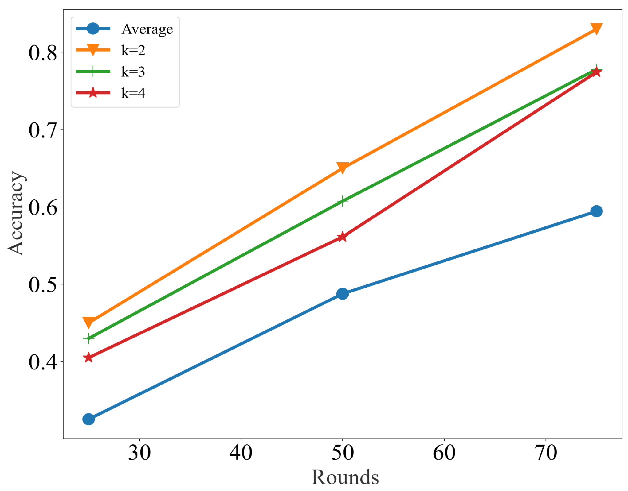
We used the Chung dataset to go through the algorithm and repeat the whole process ten times, and we took the average of ten different output results as the final accuracy of the model. To testify that the fusion effect when using two matrices was the best, we used three matrices, four matrices, and the average accuracy of fusing one matrix to nine matrices. Then, we recorded the classification accuracy of training for 25, 50, and 75 rounds, as shown in Figure 3. The experimental environment in this article was Win10 Python3.8 (Anaconda3), the CPU was an AMD R5 3600, the memory size was 32 GB, and the GPU was an NVIDIA GTX2070s (8G).
In Figure 3, the horizontal axis represents the training rounds, and the vertical axis represents the classification accuracy. k represents the number of fused matrices. It can be explicitly seen in Figure 3 that when the training reached 25 rounds, the accuracy of using two fused matrices was slightly higher than that of using three or four fusions matrices, and the average accuracy was the lowest. When training for 75 rounds, the classification accuracy obtained when using two fusion matrices was 82.2 % , which was more than 5 % higher than that when using three and four fusion matrices, and this was much higher than the average level of matrix fusions. We found that excessive matrix fusion could not reflect the features of the matrix well. On the contrary, the features when fusing many matrices became disordered and the efficiency became worse. From Section 2.6, we know that the two matrices to be fused have the highest similarity, indicating that the two matrices have the most common characteristics.
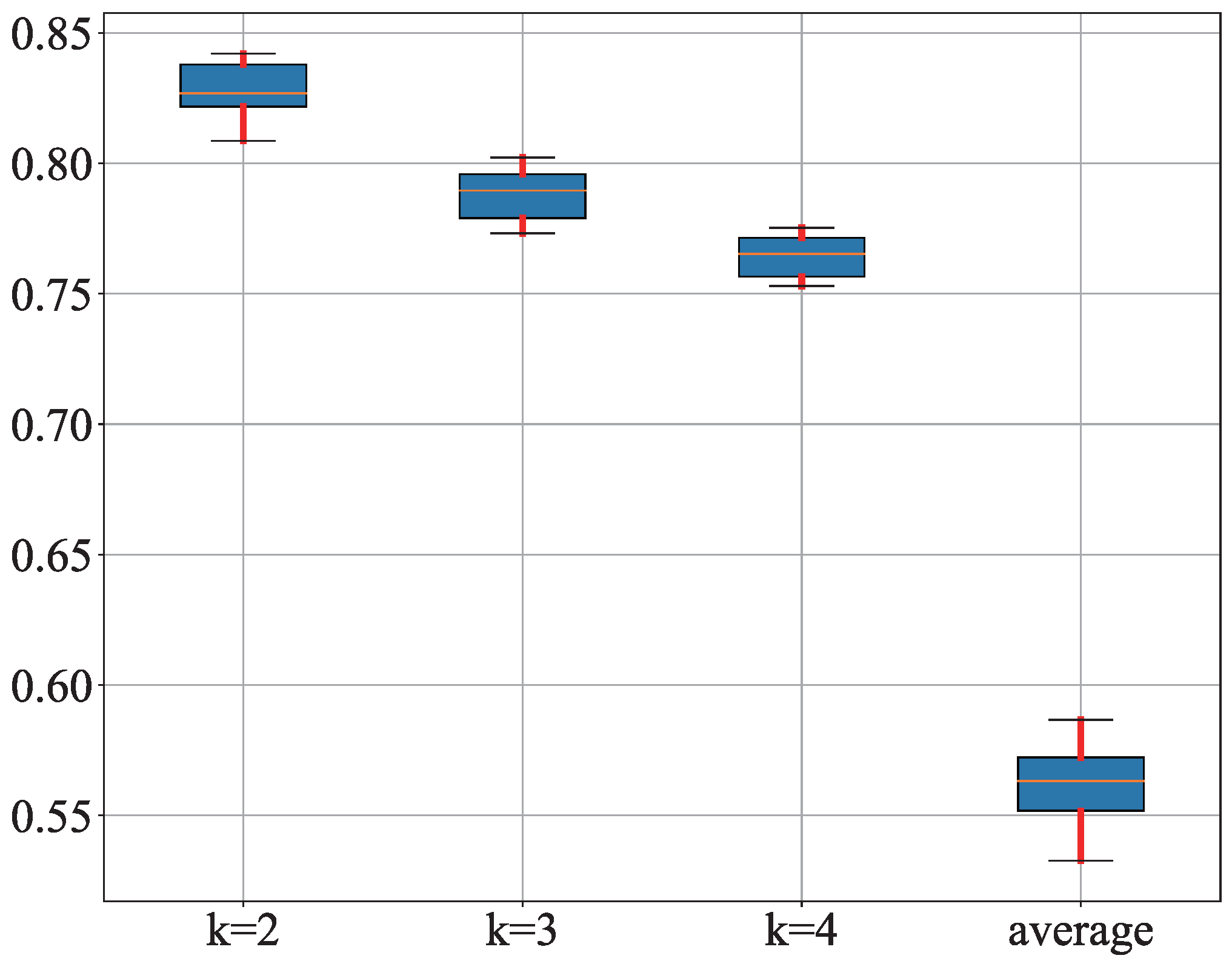
To verify the reliability of the experimental results, we repeated the above experiments 10 times and obtained a box plot of the experimental accuracy with the running rounds, as shown in Figure 4, where the horizontal axis represents the number of matrix fusions and the vertical axis represents the classification accuracy. From Figure 4, we can conclude that the cell classification accuracy obtained by using the fusion of the two matrices was the highest, and mean and quantile were also much higher than those obtained with other methods. The mean, maximum, and minimum values of the box plots obtained when using the three fusion matrices were slightly higher than the results obtained using the four fusion matrices.

3.2. Discussion

We tested the classification accuracy when fusing different matrices from four other datasets. In the Chu dataset, which is shown in Figure 5, the highest accuracy was nearly 97 % when using the fusion of two matrices; this was 1–2% higher than that obtained when using three-matrix fusion and much higher than those of the four-matrix fusion and average fusion. In the Patel, Xin, and Ning datasets, the classification accuracy of the fusion of two matrices was also significantly higher than those of the other numbers of matrices.
We also compared the SCAFG with four common semi-supervised learning algorithms, namely, label propagation, label spreading, self-training, and a GCN. Their classification accuracies on the five different datasets (see Table 1) with 25, 50, and 75 rounds are shown in Table 2.
From Table 2, we can see that for the Chung dataset, the label spreading was more accurate than label propagation and self-training before 50 rounds. Even though label spreading is similar to the basic label propagation algorithm, label spreading uses an affinity matrix based on the normalized graph Laplacian and soft clamping across the labels. When it ran for 75 rounds, the GCN surpassed all three methods and was second only to the SCAFG in accuracy. This may have been due to the fact that graph convolutional neural networks exploit deeper features between cells through convolution. For the other four datasets (Chu, Patel, Xin, and Ning), the accuracy of the GCN was higher than those of label spreading, label propagation, and self-training with 25, 50, and 75 rounds. For the Chu dataset, the accuracy of the GCN was 64.2 % when running for 25 rounds, and the accuracy of the SCAFG was 70.1 % , which was 5.9 % higher than that of the GCN. When run for 75 rounds, the accuracy of the SCAFG was 96.4 % , which was higher than that of the GCN by 7.2 % . This is because the SCAFG fused two cell matrices, which could better represent the features between cells than using a single cell matrix. Overall, the average accuracy of the SCAFG was 5–10% higher than that of the GCN, and it was better than those of the other semi-supervised methods. For the Ning dataset, the SCAFG achieved a 97.6 % classification accuracy after 75 rounds of training. Notably, the SCAFG was the most accurate method in semi-supervised cell recognition.

4. Conclusions

With the rapid development of single-cell sequencing technology, the scale of cells is also increasing. We are faced with the challenge of a large number of cells and a high feature dimension, so it is a time-consuming task to gradually identify their categories. Therefore, some semi-supervised learning algorithms were developed to solve this problem.
In this study, we proposed a semi-supervised classification algorithm, the SCAFG. We used PsiNorm to normalize the single-cell data, which made the distribution of cells more uniform; then, we used threshold segmentation to divide the cell connection features under different distributions, used the similarity distance to measure the similarity between matrices, and used matrix fusion to take full advantage of the information between matrices to reduce data redundancy. Finally, the experimental results on different sizes of single-cell datasets showed that the SCAFG had better performance than that of other methods, and that it is a robust single-cell semi-supervised classification algorithm that can be widely used.
At the same time, we think that the SCAFG can be improved in some areas. Firstly, under the existing experimental conditions, saving graphs will take some time and memory, which will affect the efficiency of the algorithm. Perhaps, we can consider using distributed technology to store graphs. Secondly, the fusion of two matrices does not necessarily have the highest accuracy, but only the highest similarity. We will continue to pay attention to these issues in the future and look forward to achieving some breakthrough solutions and promising results.

Author Contributions

Data curation, H.P.; Methodology, H.P. and Y.L.; Software, H.P.; Supervision, Y.L. and W.Z.; Writing—original draft, H.P., Y.L. and W.Z. All authors have read and agreed to the published version of the manuscript.

Funding

This work was supported by the National Natural Science Foundation of China (Grant Nos.12001408, 12161039) and the Natural Science Foundation of Jiangxi Province (20212ACB211002).

Institutional Review Board Statement

Not applicable.

Informed Consent Statement

Not applicable.

Data Availability Statement

The data used to support the findings of this study can be downloaded from https://www.ncbi.nlm.nih.gov/geo/, access on 2 June 2022. The code of the paper can be found in https://github.com/phnawa/Bioinformatics/tree/main/Semisupervised/SCAFG/Code, access on 11 June 2022.

Conflicts of Interest

The authors declare no conflict of interest.

References

  1. Bissell, M.J.; Hall, H.G.; Parry, G. How does the extracellular matrix direct gene expression? J. Theor. Biol. 1982, 99, 31–68. [Google Scholar] [CrossRef]
  2. Barry, F.; Boynton, R.E.; Liu, B.; Murphy, J.M. Chondrogenic differentiation of mesenchymal stem cells from bone marrow: Differentiation-dependent gene expression of matrix components. Exp. Cell Res. 2001, 268, 189–200. [Google Scholar] [CrossRef] [PubMed]
  3. Li, Y.; Luo, P.; Lu, Y.; Wu, F.X. Identifying cell types from single-cell data based on similarities and dissimilarities between cells. BMC Bioinform. 2021, 22, 1–18. [Google Scholar] [CrossRef] [PubMed]
  4. Grira, N.; Crucianu, M.; Boujemaa, N. Unsupervised and semi-supervised clustering: A brief survey. A Rev. Mach. Learn. Tech. Process. Multimed. Content 2004, 1, 9–16. [Google Scholar]
  5. Qi, R.; Wu, J.; Guo, F.; Xu, L.; Zou, Q. A spectral clustering with self-weighted multiple kernel learning method for single-cell RNA-seq data. Brief. Bioinform. 2021, 22, bbaa216. [Google Scholar] [CrossRef]
  6. Chi, M.; Bruzzone, L. Semisupervised classification of hyperspectral images by SVMs optimized in the primal. IEEE Trans. Geosci. Remote Sens. 2007, 45, 1870–1880. [Google Scholar] [CrossRef]
  7. Odena, A. Semi-supervised learning with generative adversarial networks. arXiv 2016, arXiv:1606.01583. [Google Scholar]
  8. Rosenberg, C.; Hebert, M.; Schneiderman, H. Semi-supervised self-training of object detection models. In Proceedings of the 2005 Seventh IEEE Workshops on Applications of Computer Vision (WACV/MOTION’05), Breckenridge, CO, USA, 5–7 January 2005. [Google Scholar]
  9. Blum, A.; Mitchell, T. Combining labeled and unlabeled data with co-training. In Proceedings of the Eleventh Annual Conference on Computational Learning Theory, Madison, WI, USA, 24–26 July 1998; pp. 92–100. [Google Scholar]
  10. Tian, F.; Gao, B.; Cui, Q.; Chen, E.; Liu, T.Y. Learning deep representations for graph clustering. In Proceedings of the AAAI Conference on Artificial Intelligence, Québec, QC, Canada, 27–31 July 2014; Volume 28. [Google Scholar]
  11. Schaeffer, S.E. Graph clustering. Comput. Sci. Rev. 2007, 1, 27–64. [Google Scholar] [CrossRef]
  12. Vapnik, V. Principles of risk minimization for learning theory. Adv. Neural Inf. Process. Syst. 1991, 4, 832–838. [Google Scholar]
  13. Fan, W.; Peng, H.; Luo, S.; Fang, C.; Li, Y. SCEC: A novel single-cell classification method based on cell-pair ensemble learning. In Proceedings of the International Conference on Intelligent Computing, Shenzhen, China, 12–15 August 2021; Springer: Berlin, Germany, 2021; pp. 433–444. [Google Scholar]
  14. Valentine, G. Images of danger: Women’s sources of information about the spatial distribution of male violence. Area 1992, 24, 22–29. [Google Scholar]
  15. Lee, C.; Landgrebe, D.A. Decision boundary feature extraction for neural networks. IEEE Trans. Neural Netw. 1997, 8, 75–83. [Google Scholar]
  16. Wu, H.; Prasad, S. Semi-supervised deep learning using pseudo labels for hyperspectral image classification. IEEE Trans. Image Process. 2017, 27, 1259–1270. [Google Scholar] [CrossRef]
  17. Wang, W.; Tan, H.; Sun, M.; Han, Y.; Chen, W.; Qiu, S.; Zheng, K.; Wei, G.; Ni, T. Independent component analysis based gene co-expression network inference (ICAnet) to decipher functional modules for better single-cell clustering and batch integration. Nucleic Acids Res. 2021, 49, e54. [Google Scholar] [CrossRef]
  18. Son, N.H. From optimal hyperplanes to optimal decision trees. Fundam. Inform. 1998, 34, 145–174. [Google Scholar] [CrossRef]
  19. Yao, X. Evolving artificial neural networks. Proc. IEEE 1999, 87, 1423–1447. [Google Scholar]
  20. Gregory, S. Finding overlapping communities in networks by label propagation. New J. Phys. 2010, 12, 103018. [Google Scholar] [CrossRef]
  21. Cui, W.; Zhou, H.; Qu, H.; Wong, P.C.; Li, X. Geometry-based edge clustering for graph visualization. IEEE Trans. Vis. Comput. Graph. 2008, 14, 1277–1284. [Google Scholar] [CrossRef]
  22. Kipf, T.N.; Welling, M. Semi-supervised classification with graph convolutional networks. arXiv 2016, arXiv:1609.02907. [Google Scholar]
  23. Li, Q.; Han, Z.; Wu, X.M. Deeper insights into graph convolutional networks for semi-supervised learning. In Proceedings of the Thirty-Second AAAI Conference on Artificial Intelligence, New Orleans, LA, USA, 2–7 February 2018. [Google Scholar]
  24. Yan, S.; Xiong, Y.; Lin, D. Spatial temporal graph convolutional networks for skeleton-based action recognition. In Proceedings of the Thirty-Second AAAI Conference on Artificial Intelligence, New Orleans, LA, USA, 2–7 February 2018. [Google Scholar]
  25. Peng, H.; Fan, W.; Fang, C.; Gao, W.; Li, Y. SCMAG: A Semisupervised Single-Cell Clustering Method Based on Matrix Aggregation Graph Convolutional Neural Network. Comput. Math. Methods Med. 2021, 2021, 6842752. [Google Scholar] [CrossRef]
  26. Chung, W.; Eum, H.H.; Lee, H.O.; Lee, K.M.; Lee, H.B.; Kim, K.T.; Ryu, H.S.; Kim, S.; Lee, J.E.; Park, Y.H.; et al. Single-cell RNA-seq enables comprehensive tumour and immune cell profiling in primary breast cancer. Nat. Commun. 2017, 8, 1–12. [Google Scholar] [CrossRef]
  27. Chu, L.F.; Leng, N.; Zhang, J.; Hou, Z.; Mamott, D.; Vereide, D.T.; Choi, J.; Kendziorski, C.; Stewart, R.; Thomson, J.A. Single-cell RNA-seq reveals novel regulators of human embryonic stem cell differentiation to definitive endoderm. Genome Biol. 2016, 17, 1–20. [Google Scholar] [CrossRef]
  28. Patel, A.P.; Tirosh, I.; Trombetta, J.J.; Shalek, A.K.; Gillespie, S.M.; Wakimoto, H.; Cahill, D.P.; Nahed, B.V.; Curry, W.T.; Martuza, R.L.; et al. Single-cell RNA-seq highlights intratumoral heterogeneity in primary glioblastoma. Science 2014, 344, 1396–1401. [Google Scholar] [CrossRef]
  29. Xin, Y.; Kim, J.; Okamoto, H.; Ni, M.; Wei, Y.; Adler, C.; Murphy, A.J.; Yancopoulos, G.D.; Lin, C.; Gromada, J. RNA sequencing of single human islet cells reveals type 2 diabetes genes. Cell Metab. 2016, 24, 608–615. [Google Scholar] [CrossRef]
  30. Leng, N.; Chu, L.F.; Barry, C.; Li, Y.; Choi, J.; Li, X.; Jiang, P.; Stewart, R.M.; Thomson, J.A.; Kendziorski, C. Oscope identifies oscillatory genes in unsynchronized single-cell RNA-seq experiments. Nat. Methods 2015, 12, 947–950. [Google Scholar] [CrossRef]
  31. Borella, M.; Martello, G.; Risso, D.; Romualdi, C. PsiNorm: A scalable normalization for single-cell RNA-seq data. Bioinformatics 2022, 38, 164–172. [Google Scholar] [CrossRef]
  32. Huang, A. Similarity measures for text document clustering. In Proceedings of the Sixth New Zealand Computer Science Research Student Conference (NZCSRSC2008), Christchurch, New Zealand, 14–18 April 2008; Volume 4, pp. 9–56. [Google Scholar]
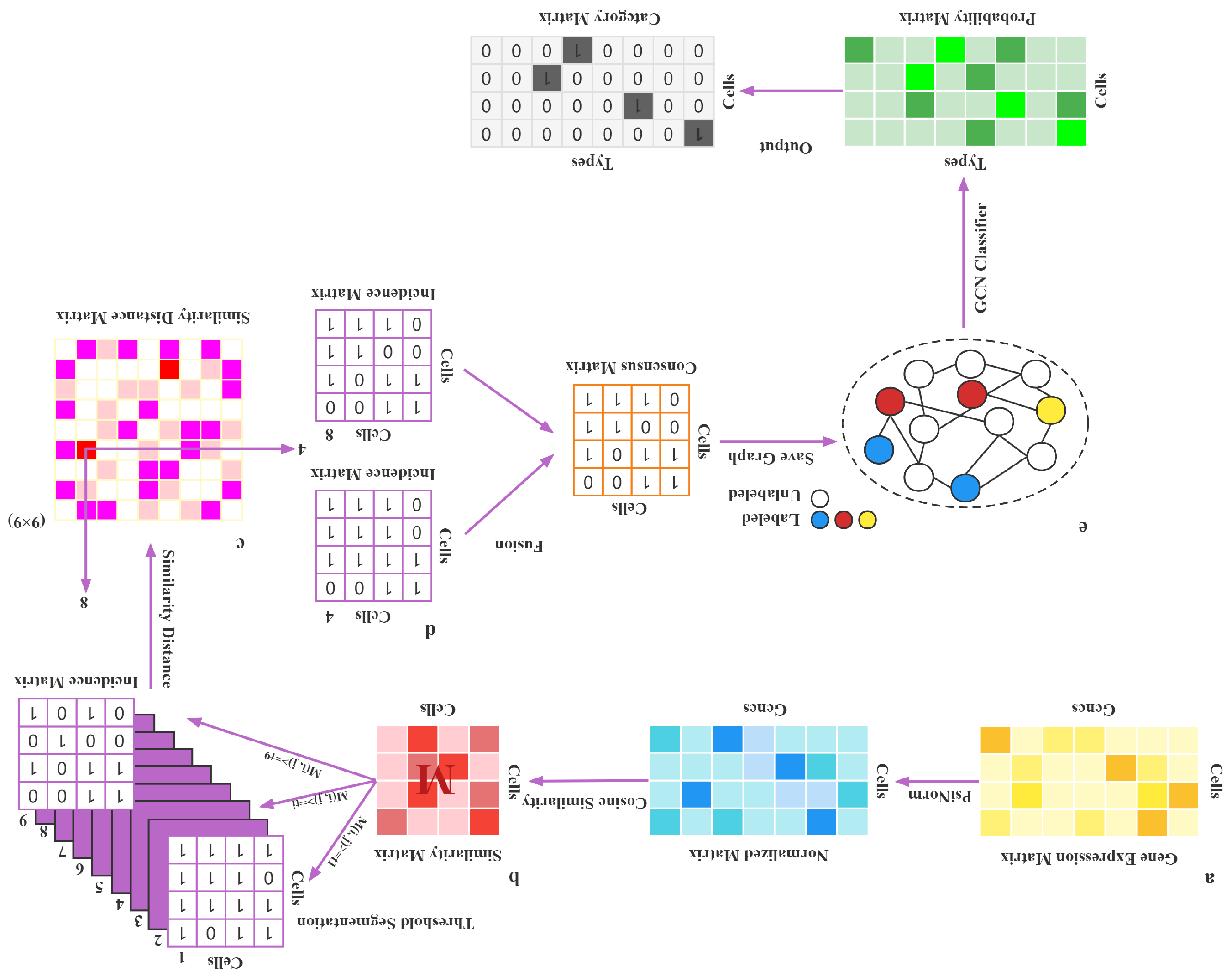
Figure 1. Overview of the SCAFG. (a) Data preprocessing, including normalization and similarity transformation of the gene expression matrix. (b) Dividing the similarity matrix into nine incidence matrices through threshold segmentation, then converting the similarities between the incidence matrices into a similarity distance matrix. (c) Finding the row and column index of the largest element value in the similarity distance matrix. (d) Fusing the incidence matrix and saving the consensus matrix as a graph. (e) The graph is the input of the GCN, and the output is a probability matrix. The column index corresponding to the maximum probability value of each row in the probability matrix is the category to which the cell belongs.
Mathematics 10 03407 g001
Figure 2. Structure of the graph convolutional neural network structure.
Mathematics 10 03407 g002
Figure 3. The classification accuracy of the Chung dataset with different numbers of matrices being fused.
Mathematics 10 03407 g003
Figure 4. The box plot of the Chung dataset, recording the highest accuracy for each of the 10 experiments.
Mathematics 10 03407 g004
Figure 5. Box plots for four datasets—comparison of the classification accuracies with fusion of different matrices: (a) Chu, (b) Patel, (c) Xin, and (d) Ning.
Mathematics 10 03407 g005
Table 1. Key information of the five datasets.
DatasetsNumber of CellsClassNumber of GenesData SourcesReferences
Chung5631357915GSE75688Chung et al. [26].
Chu1018719097GSE75748Chu et al. [27]
Patel43065948GSE57872Patel et al. [28].
Xin1600839851GSE81608Xin et al. [29].
Ning460419084GSE64016Ning et al. [30].
Table 2. The performance of different semi-supervised methods.
DatasetIterationLabel PropagationLabel SpreadingSelf-TrainingGCNSCAFG
2536.647.536.632.346.4
Chung5044.656.149.844.664.2
7547.759.254.258.882.2
2544.153.258.864.270.1
Chu5058.355.669.586.792.3
7561.556.973.289.296.4
2550.646.249.765.176.7
Patel5067.158.359.473.889.9
7570.664.865.277.696.3
2570.264.660.180.987.4
Xin5076.274.568.582.288.1
7580.174.874.283.691.2
2551.256.746.882.691.1
Ning5058.469.263.185.493.3
7562.474.669.289.897.6
Publisher’s Note: MDPI stays neutral with regard to jurisdictional claims in published maps and institutional affiliations.