Article

Improved Estimation of the Inverted Kumaraswamy Distribution Parameters Based on Ranked Set Sampling with an Application to Real Data

1
Faculty of Graduate Studies for Statistical Research, Cairo University, Giza 12613, Egypt
2
Department of Mathematics, Faculty of Science, Al Al-Bayt University, Mafraq 25113, Jordan
3
Department of Mathematical Sciences, College of Science, Princess Nourah bint Abdulrahman University, P.O. Box 84428, Riyadh 11671, Saudi Arabia
*
Authors to whom correspondence should be addressed.
Mathematics 2022, 10(21), 4102; https://doi.org/10.3390/math10214102
Submission received: 16 September 2022 / Revised: 17 October 2022 / Accepted: 31 October 2022 / Published: 3 November 2022

Abstract

:
The ranked set sampling (RSS) methodology is an effective technique of acquiring data when measuring the units in a population is costly, while ranking them is easy according to the variable of interest. In this article, we deal with an RSS-based estimation of the inverted Kumaraswamy distribution parameters, which is extensively applied in life testing and reliability studies. Some estimation techniques are regarded, including the maximum likelihood, the maximum product of spacing’s, ordinary least squares, weighted least squares, Cramer–von Mises, and Anderson–Darling. We demonstrate a simulation investigation to assess the performance of the suggested RSS-based estimators via accuracy measures relative to simple random sampling. On the basis of actual data regarding the waiting times between 65 consecutive eruptions of Kiama Blowhole, additional conclusions have been drawn. The outcomes of simulation and real data application demonstrated that RSS-based estimators outperformed their simple random sampling counterparts significantly based on the same number of measured units.

1. Introduction

In some investigations, cost-effective sampling is a key concern, particularly when the measurement of the characteristic of interest is expensive, uncomfortable, or time-consuming. In order to increase the accuracy achieved per unit of the sample, the ranked set sampling (RSS) approach is an excellent tool for achieving observational economy. Reference [1] proposed the RSS technique as an alternative to the frequently used simple random sample (SRS) methodology for increasing the efficiency of the sample mean. In RSS, the population is divided into q sets of q units each by randomly selecting q2 units from it. Without taking actual measurements, the q units in each set are ranked with respect to the study variable. For actual quantification, the lowest-ranked unit from the first set of q units is chosen. The second smallest ranked unit is measured from the second set of q units. The process is repeated; say h times until the greatest rated unit from the last set is determined. To obtain an RSS sample of size n = qh, the entire process can be replicated a number of times, say h times. The following matrix notation is considered to express the RSS design.
I n i t i a l O b s e r v a t i o n s X ( 1 : 1 ) X ( 1 : 2 ) X ( 1 : q ) X ( 2 : 1 ) X ( 2 : 2 ) X ( 2 : q ) X ( q : 1 ) X ( q : 2 ) X ( q : q ) R a n k e d O b s e r v a t i o n s X 11 X 21 X q 1 X 12 X 22 X q 2 X 1 q X 2 q X q q R S S ( h = 1 ) X 11 , X 22 , , X q q
The mathematical foundation of RSS was initially created in reference [2]. In statistical inference, the parametric estimate approach employing the RSS sampling strategy is of utmost importance. A large number of studies have recently been conducted on the issue of RSS-based estimate for a variety of parametric models. For example, refeference [3] used the data from the RSS technique to calculate the population variance. In subsequent years, RSS was employed to estimate the statistical distribution’s involved parameters. Reference [4] used RSS to estimate the exponential distribution parameters, while reference [5] investigated the estimator of the Cauchy distribution’s location parameter. Reference [6] looked at estimating normal and exponential distribution parameters based on RSS. Reference [7] investigated estimators for the logistic distribution’s location and scale parameters, whereas reference [8] considered the RSS to get the geometric parameter estimators. Reference. [9] succeeded in estimating the parameters of the half-logistic distribution, while reference. [10] investigated estimators of logistic distribution parameters using RSS. Reference [11] achieved estimating modified Weibull distribution parameters. Reference [12] used RSS to derive maximum likelihood (ML) and Bayesian estimators for generalized exponential model. Reference [13] handled with parameter estimators of Pareto distribution using RSS. The parameter estimator of the Rayleigh distribution was regarded in [14] using different methods of estimations and ranking designs. Within the framework of RSS, reference [15] examined the approach of the ML for the shape and scale parameters of the generalized Rayleigh distribution. Reference [16] considered estimation of the new Weibull-Pareto distribution parameters using RSS. Reference [17] discussed the parameter estimators of Zubair Lomax distribution using RSS. Reference [18] investigated efficient estimation of the generalized quasi-Lindley distribution parameters under RSS. For recent results and references, see [19,20,21,22,23,24,25,26,27].
The Kumaraswamy distribution (KD) was offered in [28], which is one of the most significant lifetime distributions with a range of [0,1]. It cannot, however, be utilized for most lifetime data sets that theoretically have limitless support. It is regarded as a viable alternative to beta distribution since they both share the same characteristics such as being uni-modal, decreasing, increasing, or constant. The KD’s probability density function (PDF) with two positive shape parameters is defined by:
f ( x ; τ , υ ) = τ υ x τ 1 1 x τ υ 1 ; τ , υ > 0 , 0 < x < 1 .
Reference [29] proposed the inverted KD distribution (IKD) with the goal of providing a new flexible lifetime distribution for analyzing real data sets in the best situation. The following are indeed the principles of the IKD: It’s the distribution of the random variable Z = 1/X − 1, where 
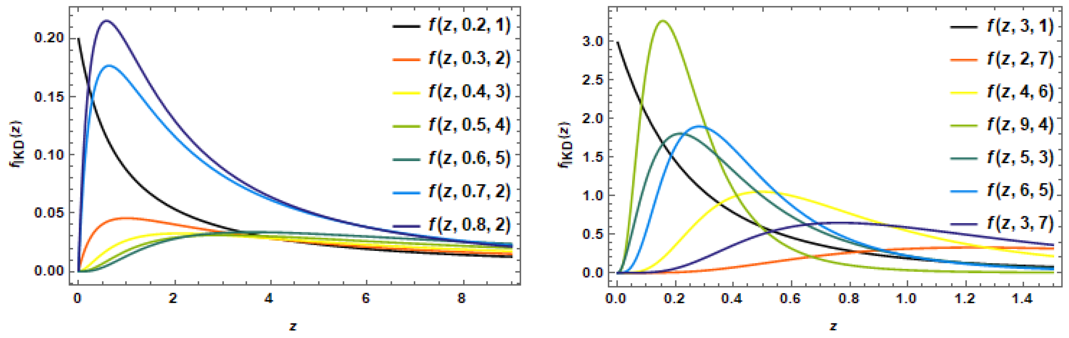
X is a random variable following the KD in Equation (1). The PDF and cumulative distribution function (CDF) of the IKD are, respectively, characterized by:
f ( z ; τ , υ ) = τ υ ( 1 + z ) τ 1 1 1 + z τ υ 1 ; z , τ , υ > 0 ,
F ( z ; τ , υ ) = 1 1 + z τ υ ; z , τ , υ > 0 .
Figure 1 presents some possible PDF plots of the IKD for some selected distribution parameters. It is clear that the distribution is skewed to the right.
The CDF (3) comprises several well-known distributions, including (i) the Lomax distribution for υ = 1 , (ii) the beta type II (inverted beta) distribution for τ = 1 , (iii) log-logistic distribution for τ = υ = 1 , (iv) the inverse Weibull distribution as υ , and the generalized exponential distribution when τ . According to reference [29], the IKD has a long right tail, and when compared to other distributions, the IKD gives optimistic forecasts of uncommon events happening in the right tail.
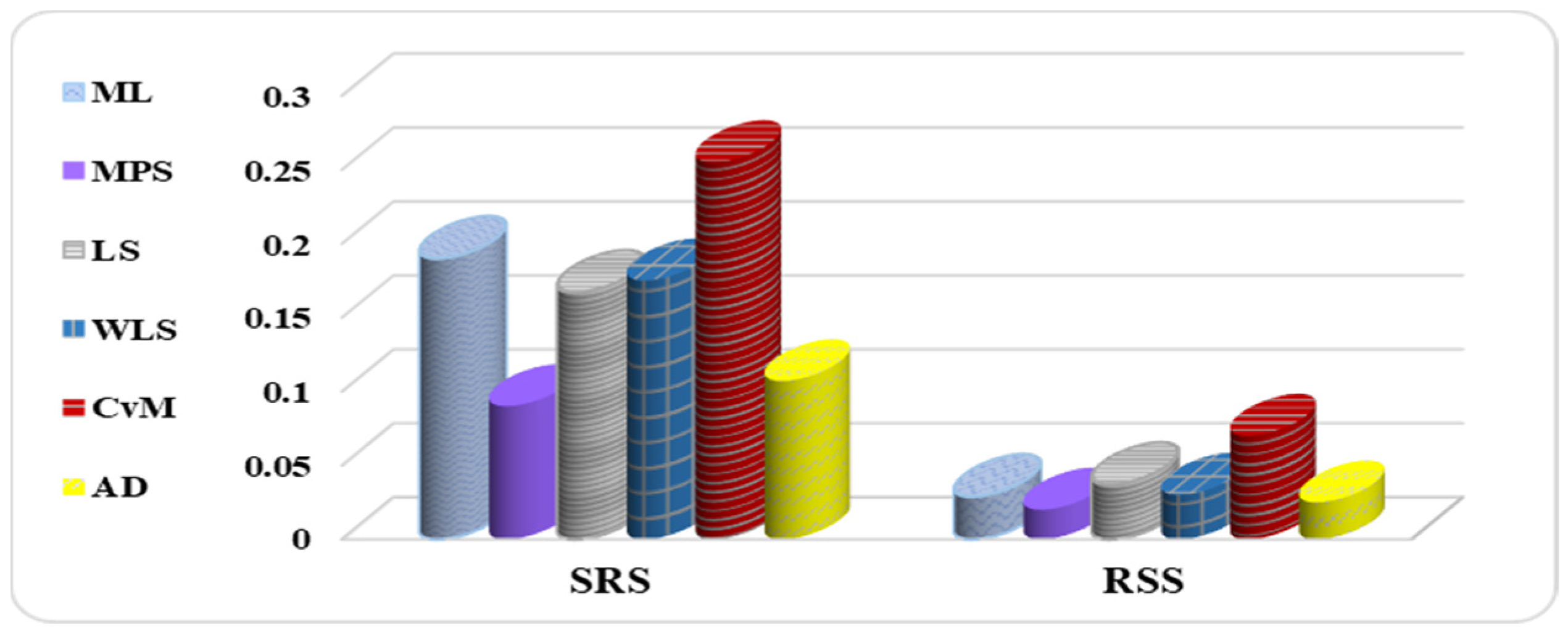
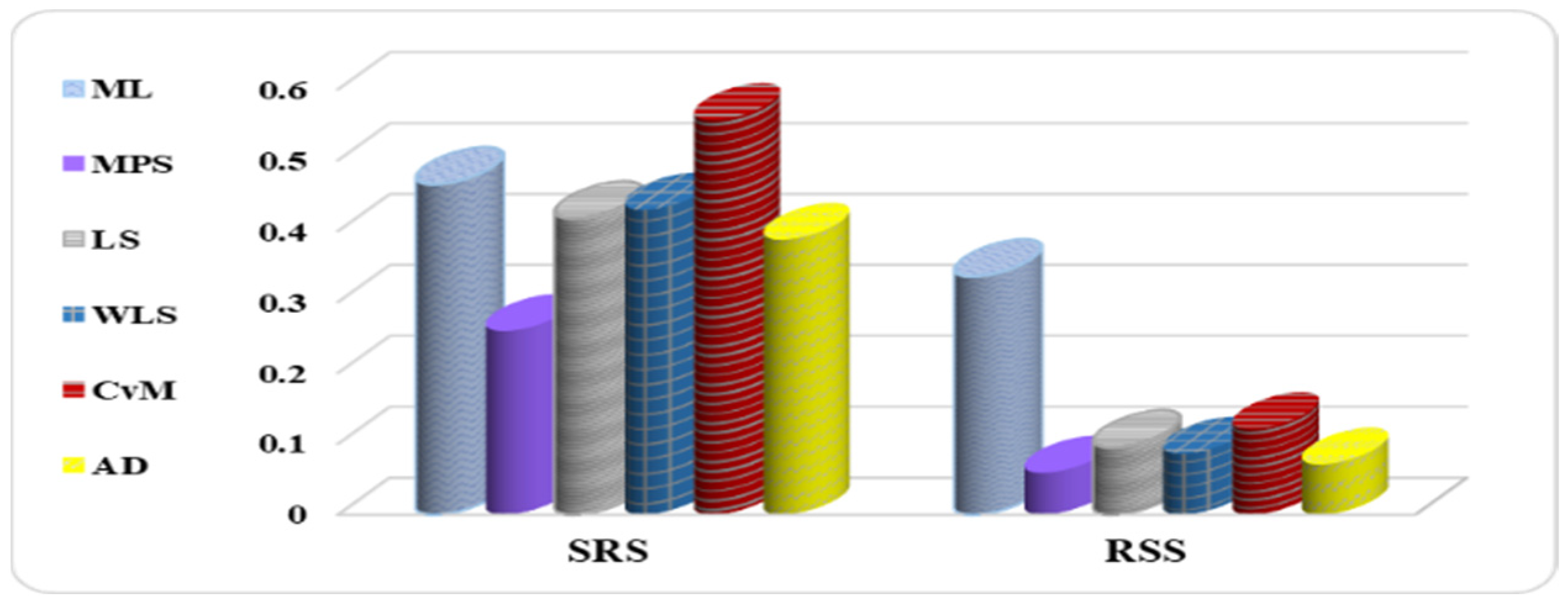
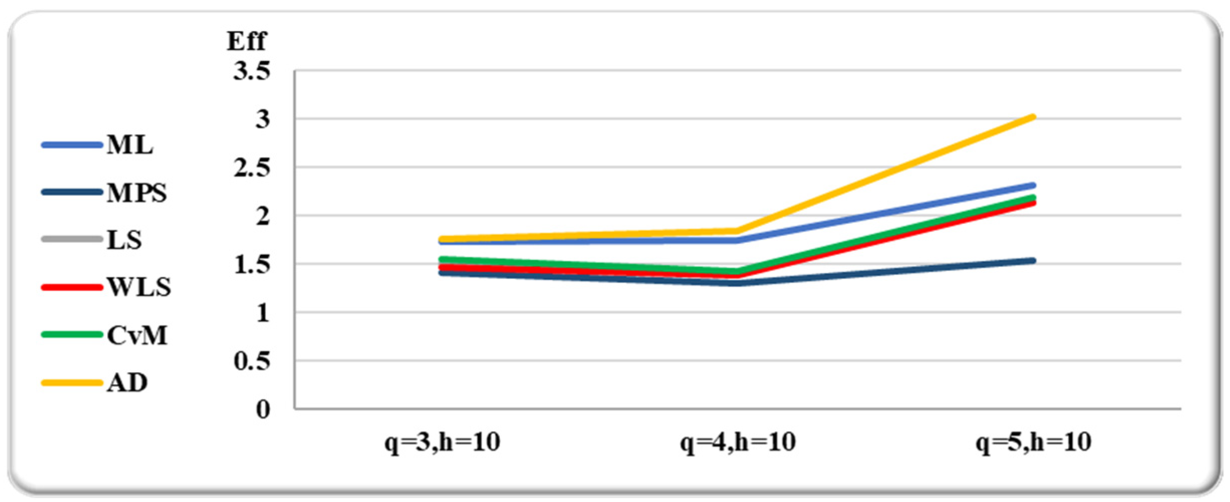
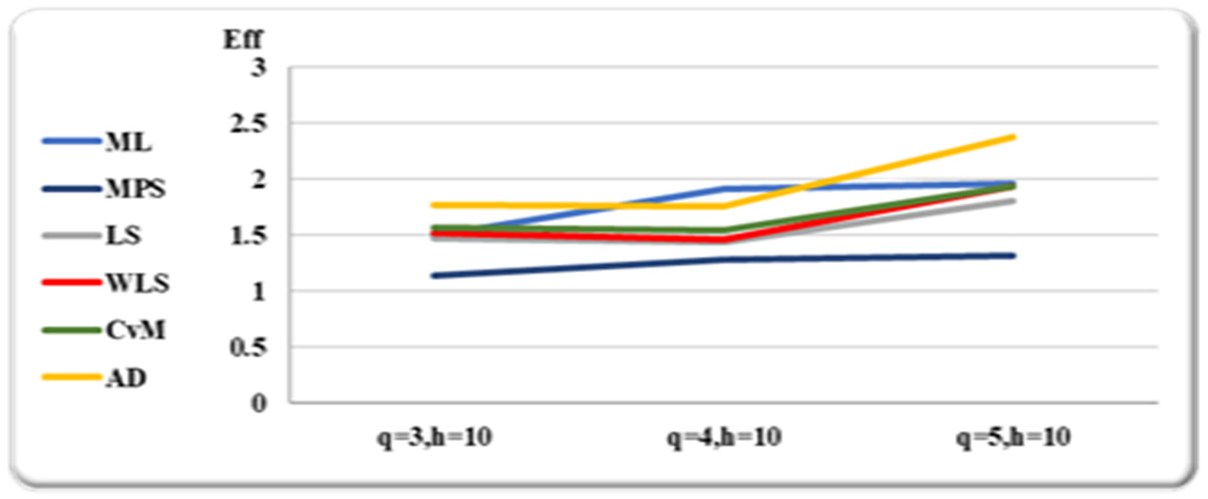
To our knowledge, there have been no published works that have utilized the RSS to estimate IKD parameters. In this study, we assumed that the ranking is perfect and we focus on several classical estimations of the IKD parameters using RSS and SRS. The considered methods are the ML, maximum product of spacing (MPS), least squares (LS), weighted least squares (WLS), Cramer–von Mises (CvM), and Anderson–Darling (AD). A simulation study compares the suggested RSS based estimators to the basic SRS based on some criteria measures.
The following is the paper’s configuration: we provide the ML estimators (MLEs) and MPS estimators (MPSEs) of the IKD parameters in Section 2. Section 3 obtains the IKD parameter estimators using LS and WLS approaches. Using the AD and CvM methodologies, we obtain the IKD parameter estimators in Section 4. Section 5 and Section 6 describe, respectively, simulation research as well as its application to real-world situations, and comparing RSS estimators to SRS equivalents. The paper comes to a close with main findings in Section 7.

2. ML and MPS Methods of Estimation

The ML and MPS estimation methods are examined in this section for estimating the IKD parameters. First, we’ll go through the RSS framework methodology, and then obtain the estimators from SRS.

2.1. ML Estimators

Let { Z c t , c = 1 , 2 , , q , t = 1 , 2 , , h } denote cth order statistics (OS) in the tth cycle, where h is the number of cycles and q is the set size. The data in RSS are all mutually independent, and the data are distributed identically for each c = 1 ,   2 , , q . The distribution of the cth data, for each c = 1 ,   2 , ,   q , is identical to the distribution of the cth OS of the random sample X1, X2, …, Xq, that is;
f Z c t ( z c t ) = q ! ( c 1 ) ! ( q c ) ! f ( z c t ) F ( z c t ) c 1 1 F ( z c t ) q c , < z < .
Substituting Equations (2) and (3) in Equation (4), then we have:
f Z c t ( z ) = ( q ) ! τ υ ( c 1 ) ! ( q c ) ! ( 1 + z c t ) τ 1 1 1 + z c t τ υ c 1 1 1 1 + z c t τ υ q c , 0 < z c t < .
The likelihood function of IKD using RSS { Z c t , c = 1 , 2 , , q , t = 1 , 2 , , h } , where n = q h is the sample size, is as follows:
l S S ( z ) = c = 1 q t = 1 h ( q ) ! τ υ ( c 1 ) ! ( q c ) ! ( 1 + z c t ) τ 1 1 ( 1 + z c t ) τ υ c 1 1 1 1 + z c t τ υ q c .
The log-likelihood function of IKD, denoted by l S S * is as follows:
l S S * q h ln ( τ υ ) ( τ + 1 ) c = 1 q t = 1 h ln ( ξ c t ) + ( υ c 1 ) c = 1 q t = 1 h ln ( 1 ξ c t τ ) + ( q c ) c = 1 q t = 1 h ln 1 1 ξ c t τ υ ,
where ξ c t = ( 1 + z c t ) . The MLEs of τ , and υ , denoted by τ ^ ML , and υ ^ ML , of the IKD using RSS are produced by solving the nonlinear equations
l S S * / τ = 0 , and   l S S * / υ = 0 .
Let Z 1 , Z 2 , , Z n be a SRS of size n from a IKD with PDF (2) and CDF (3). The log-likelihood function, say l S R S * , for τ and υ is given by:
l S R S * = n ln τ + n ln υ ( τ + 1 ) i = 1 n ln 1 + z i + ( υ 1 ) i = 1 n ln 1 1 + z i τ .
The MLEs for τ and υ , say τ ˜ M L and υ ˜ M L , are given as the solution of the following equations:
l S R S * / τ = 0 , and   l S R S * / υ = 0 .
Using numerical technique in Equation (7), we obtain the MLEs of τ and υ , denoted by τ ˜ ML and υ ˜ ML .

2.2. MPS Estimators

For estimating the population parameters of continuous distributions, reference [30] presented a powerful alternative approach known as MPS. Consider the ordered items Z ( 1 : n ) , Z ( 2 : n ) , , Z ( n : n ) constitute a RSS of size n = q h , q is set size and h is the cycle numbers drawn from a distribution Equation (3). Hence, the uniform spacing’s are defined by D c ( τ , υ ) = F z ( c : n ) τ , υ F z ( c 1 : n ) τ , υ , c = 1 , 2 , , n + 1 , with F z ( 0 : n ) τ , υ = 0 , F z ( n + 1 : n ) τ , υ = 1 , such that c = 1 n + 1 D c ( τ , υ ) = 1 . The MPSEs, represented by τ ^ MPS , υ ^ MPS , are obtained by maximizing the geometric mean of the spacing GM ( τ , υ ) , where
GM ( τ , υ ) = c = 1 n + 1 D c ( τ , υ ) 1 / ( n + 1 ) .
The logarithm of (8), denoted by GM ( τ , υ ) , is
GM ( τ , υ ) = 1 n + 1 c = 1 n + 1 ln 1 1 + z ( c : n ) τ υ 1 1 + z ( c 1 : n ) τ υ .
The MPSEs; τ ^ MPS , υ ^ MPS can also be obtained by solving the nonlinear equations numerically:
GM ( τ , υ ) υ = 1 n + 1 c = 1 n + 1 1 D c τ , υ Υ 1 z ( c : n ) τ , υ Υ 1 z ( c 1 : n ) τ , υ = 0 ,
GM ( τ , υ ) τ = 1 n + 1 c = 1 n + 1 1 D c τ , υ Υ 2 z ( c : n ) τ , υ Υ 2 z ( c 1 : n ) τ , υ = 0 ,
where
Υ 1 z ( c : n ) τ , υ = υ 1 1 + z ( c : n ) τ υ = 1 1 + z ( c : n ) τ υ ln 1 1 + z ( c : n ) τ ,
Υ 2 z ( c : n ) τ , υ = τ 1 1 + z ( c : n ) τ υ = υ 1 1 + z ( c : n ) τ υ 1 1 + z ( c : n ) τ ln 1 + z ( c : n ) .
Based on SRS, let Z ( 1 ) , Z ( 2 ) , , Z ( n ) be the OS from a sample of size n from Equation (3). Hence, the uniform spacing’s in this case are defined by D i ( τ , υ ) = F z ( i ) τ , υ F z ( i 1 ) τ , υ , i = 1 , 2 , , n + 1 with F z ( 0 ) τ , υ = 0 , F z ( n + 1 ) τ , υ = 1 , such that i = 1 n + 1 D i ( τ , υ ) = 1 . The MPSEs, represented by τ ˜ MPS , υ ˜ MPS , are obtained by maximizing the geometric mean of the spacing GM S R S ( τ , υ ) , where
GM S R S ( τ , υ ) = i = 1 n + 1 D i ( τ , υ ) 1 / ( n + 1 ) .
The logarithm of Equation (13), denoted by GM S R S ( τ , υ ) , is
GM S R S ( τ , υ ) = 1 n + 1 i = 1 n + 1 ln 1 1 + z ( i ) τ υ 1 1 + z ( i 1 ) τ υ .
The MPSEs; τ ^ MPS , υ ^ MPS can also be obtained by solving the following nonlinear equations numerically:
GM S R S ( τ , υ ) υ = 1 n + 1 i = 1 n + 1 1 D i τ , υ Υ 1 z ( i ) τ , υ Υ 1 z ( i 1 ) τ , υ = 0 ,
GM S R S ( τ , υ ) τ = 1 n + 1 i = 1 n + 1 1 D i τ , υ Υ 2 z ( i ) τ , υ Υ 2 z ( i 1 ) τ , υ = 0 ,
where, Υ 1 z ( i ) τ , υ and Υ 2 z ( i ) τ , υ have the same expressions as Equations (11) and (12) by replacing z ( c : n ) with z ( i ) .

3. LS and WLS Methods

The LS and WLS methods for estimating unknown parameters are well established in reference [31]. Here, the LS estimators (LSEs) and WLS estimators (WLSEs) of τ , and υ are examined using SRS and RSS design. We’ll go over the RSS framework technique first, and then obtain these estimators using SRS.
Let the ordered items Z ( 1 : n ) , Z ( 2 : n ) , , Z ( n : n ) constitute a RSS of size n = q h , from the IKD has the CDF given by Equation (3). The LSEs and WLSEs of τ , and υ , are derived by minimizing the following functions with respect to population parameters:
= c = 1 n F z ( c : n ) τ , υ c n + 1 2 = c = 1 n 1 1 + z ( c : n ) τ υ c n + 1 2 ,
= c = 1 n ( c , n ) F z ( c : n ) τ , υ c n + 1 2 = c = 1 n ( c , n ) 1 1 + z ( c : n ) τ υ c n + 1 2 ,
where ( c , n ) = ( n + 1 ) 2 ( n + 2 ) c ( n c + 1 ) . As an alternative to Equation (16), the following nonlinear equations can be used to yield the LSEs of τ , and υ , denoted by τ ^ LS , and υ ^ LS , respectively, as below:
υ = 2 c = 1 n 1 1 + z ( c : n ) τ υ c n + 1 Υ 1 z ( c : n ) τ , υ = 0 ,
τ = 2 c = 1 n 1 1 + z ( c : n ) τ υ c n + 1 Υ 2 z ( c : n ) τ , υ = 0 .
Similarly, as an alternative to Equation (17), the following nonlinear equations can be used to obtain the WLSEs of τ , and υ , respectively, denoted by τ ^ WLS , and υ ^ WLS , as below:
υ = 2 c = 1 n ( c , n ) 1 1 + z ( c : n ) τ υ c n + 1 Υ 1 z ( c : n ) τ , υ = 0 ,
τ = 2 c = 1 n ( c , n ) 1 1 + z ( c : n ) τ υ c n + 1 Υ 2 z ( c : n ) τ , υ = 0 ,
where Υ 1 z ( c : n ) τ , υ and Υ 2 z ( c : n ) τ , υ are defined in Equations (11) and (12).
Additionally, the LSEs and WLEs, of ordered SRS Z ( 1 ) , Z ( 2 ) , , Z ( n ) of sizes nº, for τ , and υ , denoted by τ ˜ LS , υ ˜ LS and τ ˜ WLS , υ ˜ WLS are obtained, by solving numerically the following nonlinear equations
S R S υ = 2 i = 1 n 1 1 + z ( i ) τ υ i n + 1 Υ 1 z ( i ) τ , υ = 0 ,
S R S τ = 2 i = 1 n 1 1 + z ( i ) τ υ i n + 1 Υ 2 z ( i ) τ , υ = 0 ,
S R S υ = 2 i = 1 n ( n + 1 ) 2 ( n + 2 ) i ( n i + 1 ) 1 1 + z ( i ) τ υ i n + 1 Υ 1 z ( i ) τ , υ = 0 ,
S R S τ = 2 i = 1 n ( n + 1 ) 2 ( n + 2 ) i ( n i + 1 ) 1 1 + z ( i ) τ υ i n + 1 Υ 2 z ( i ) τ , υ = 0 ,
where, Υ 1 z ( i ) τ , υ and Υ 2 z ( i ) τ , υ have the same expressions as Equations (11) and (12) by replacing z ( c : n ) with z(i), where z(i) is the ordered SRS of size n with CDF of IKD presented in Equation (3).

4. AD and CvM Methods

We employ two estimating methods that are based on the minimization of two well-known goodness-of-fit statistics. The two techniques are the CvM and AD, both of which are based on the difference between the CDF and empirical distribution function estimations. The CvM estimators (CvMEs) and AD estimators (ADEs) of the IKD are explored using SRS and RSS designs.
Suppose that Z ( 1 : n ) , Z ( 2 : n ) , , Z ( n : n ) are OS items constitute a RSS of size n = q h , from IKD. The CvMEs and ADEs of τ , and υ , are derived by minimizing the following functions with respect to population parameters
A = 1 12 n + 1 n c = 1 n F z ( c : n ) τ , υ 2 c 1 2 n 2 ,
M = n 1 n c = 1 n ( 2 c 1 ) log F z ( c : n ) τ , υ + log F ¯ z ( n c + 1 : n ) τ , υ .
As an alternative to Equation (26), the following nonlinear equations can be used to get the CvMEs of τ , and υ , denoted by τ ^ CM , and υ ^ CM , as below:
A υ = 2 n c = 1 n 1 1 + z ( c : n ) τ υ 2 c 1 2 n Υ 1 z ( c : n ) τ , υ = 0 ,
A τ = 2 n c = 1 n 1 1 + z ( c : n ) τ υ 2 c 1 2 n Υ 2 z ( c : n ) τ , υ = 0 ,
where Υ 1 z ( c : n ) τ , υ and Υ 2 z ( c : n ) τ , υ are defined in Equations (11) and (12). Similarly, as an alternative to Equation (27), the following nonlinear equations can be used to obtain the ADEs of τ , and υ , denoted by τ ^ AD , and υ ^ AD , as below:
M υ = 1 n c = 1 n ( 2 c 1 ) Υ 1 z ( c : n ) τ , υ F z ( c : n ) τ , υ Υ 1 z ( n c + 1 : n ) τ , υ F ¯ z ( n c + 1 : n ) τ , υ = 0 ,
M τ = 1 n c = 1 n ( 2 c 1 ) Υ 2 z ( c : n ) τ , υ F z ( c : n ) τ , υ Υ 2 z ( n c + 1 : n ) τ , υ F ¯ z ( n c + 1 : n ) τ , υ = 0 ,
where Υ 1 z ( c : n ) τ , υ and Υ 2 z ( c : n ) τ , υ are defined in Equations (11) and (12).
Furthermore, the ADs of τ , and υ , denoted by τ ˜ CM , and υ ˜ CM , based on ordered SRS Z ( 1 ) , Z ( 2 ) , , Z ( n ) of sizes nº are obtained by solving numerically the following equations
A S R S υ = 2 n i = 1 n 1 1 + z ( i ) τ υ 2 i 1 2 n Υ 1 z ( i ) τ , υ = 0 ,
A S R S τ = 2 n i = 1 n 1 1 + z ( i ) τ υ 2 i 1 2 n Υ 2 z ( i ) τ , υ = 0 ,
where Υ 1 z ( i ) τ , υ and Υ 2 z ( i ) τ , υ are defined in Equations (11) and (12) with ordered samples Z ( 1 ) , Z ( 2 ) , , Z ( n ) .
Similarly, the CvMEs of τ , and υ , denoted by τ ˜ CM , and υ ˜ CM , based on ordered SRS Z ( 1 ) , Z ( 2 ) , , Z ( n ) of sizes nº, are obtained by solving the following non-linear equations:
M S R S υ = 1 n i = 1 n ( i 1 ) Υ 1 z ( i ) τ , υ F z ( i ) τ , υ Υ 1 z ( n i + 1 ) τ , υ F ¯ z ( n i + 1 ) τ , υ ,
M S R S τ = 1 n i = 1 n ( 2 i 1 ) Υ 2 z ( i ) τ , υ F z ( i ) τ , υ Υ 2 z ( n i + 1 ) τ , υ F ¯ z ( n i + 1 ) τ , υ ,
where Υ 1 z ( i ) τ , υ and Υ 2 z ( n i + 1 ) τ , υ are defined in Equations (11) and (12) with ordered samples Z ( 1 ) , Z ( 2 ) , , Z ( n ) .

5. Numerical Evaluation

A simulation study is undertaken here to evaluate the performance of the estimation methods under SRS and RSS. The random samples were produced using IKD for different values of υ and τ . The following is the simulation algorithm:
  • Generate nº SRS from IKD using the quantile function z i = 1 ( u ) 1 / υ 1 / τ 1 , 0 < u < 1 ,  i = 1, 2,…, n , where u is the uniform random variable.
  • Select q random samples via SRS each set of size q from the IKD, then rank the units within each set.
  • Choose a sample for actual quantification by including the smallest ranked unit in the first set, the second smallest ranked unit in the second set, the process continues in this way until the largest ranked unit is selected from the last set.
  • Repeat steps 2 and 3 for h cycles to obtain a sample of sizes n = q h , where the set size q = 3, 4, 5 with cycles number h = 5 and 10.
  • The sample sizes of SRS are selected as n = 15, 20, 25, 30, 40, and 50. The sample sizes of RSS are selected as n = q h , where the set size q = 3, 4, 5 with cycles number h = 5 and 10.
  • The parameter values are selected as ( υ , τ ) = (0.5, 0.8), (0.5, 1.2), (1.2, 0.8) and (1.5, 1.5).
  • Obtain the ML estimates under RRS and SRS, respectively, by solving numerically Equations (6) and (7).
  • The MPS estimates of τ , and υ , are produced by solving Equations (9) and 10 for RSS, while solving Equations (14) and (15) in case of SRS.
  • The LS and WLS estimates of τ , and υ , are computed by solving numerically Equations (18)–(21) for RSS and solving Equations (22)–(25) in case of SRS.
  • The CvM and AD estimates of τ , and υ , are computed by solving numerically Equations (28)–(31) in case of SRS, while solving Equations (32)–(35) in case of SRS.
  • Repeat the pervious steps from 1 to 10 N times representing different samples, where N = 1000. The criteria for comparison include mean squared errors (MSEs) for all parameter estimates (PEs) and efficiency (Eff), which are obtained using the following relations:
    MSE ( ϑ ^ ) = 1 1000 c = 1 1000 ϑ ^ c ϑ 2 , Eff ( ϑ ^ ) = MSE SRS ( ϑ ˜ ) MSE S S ( ϑ ^ ) , ϑ ^ = τ ^ , υ ^ .
The PE, MSE, and the Eff are all presented in Table 1, Table 2, Table 3, Table 4, Table 5, Table 6, Table 7, Table 8, Table 9, Table 10, Table 11 and Table 12. One can draw the following conclusions from the simulation findings.
All estimates based on RSS are more efficient than their competitors based on SRS in most of the situations (see Table 9, Table 10, Table 11 and Table 12).
All estimates under RSS generally exhibit lower MSE than those under SRS for different sample sizes.
As the cycles number increase, the Eff value of estimates increases in most of the cases (Table 9, Table 10, Table 11 and Table 12).
In most of the cases, as seen in Figure 2 and Figure 3, the MSEs of all estimates decrease as the set size increases. Also, the MSE of υ ^ CM and τ ^ CM has the highest values, while the MSE of υ ^ MPS , υ ^ ML , τ ^ MPS and τ ^ ML has the smallest values.
Figure 2. MSE of υ estimates at ( υ , τ ) = ( 0.5 , 0.8 ) in RSS.
Mathematics 10 04102 g002
Figure 3. MSE of τ estimates at ( υ , τ )   = ( 0.5 , 0.8 ) in RSS.
Mathematics 10 04102 g003
In most of the cases, the MSEs of all estimates decrease as n increases in both SRS and RSS (see Figure 3 and Figure 4).
The MSE of υ ^ MPS , and τ ^ MPS , take the least values at ( υ , τ ) = ( 0.5 , 0.8 ) for sample sizes = 15, 20 and 25 (see Figure 4 and Figure 5).
The MSE of υ ^ CM , and τ ^ CM , get the largest values at ( υ , τ ) = ( 0.5 , 0.8 ) for sample sizes = 15, 20 and 25 in both sampling methods (see Figure 2, Figure 3, Figure 4 and Figure 5).
Figure 4. MSE of υ estimates at ( υ , τ ) = ( 0.5 , 0.8 ) in SRS.
Mathematics 10 04102 g004
Figure 5. MSE of τ estimates at ( υ , τ ) = ( 0.5 , 0.8 ) in SRS.
Mathematics 10 04102 g005
The MSEs of υ and τ estimates for all methods of estimation in RSS are smaller than the others via SRS (Figure 6 and Figure 7).
The MSEs of υ ˜ MPS and υ ^ MPS get the smallest values in both SRS and RSS schemes. While, the MSEs of υ ˜ CM and υ ^ CM get the highest values in both SRS and RSS in majority of situations.
Figure 6. MSE of υ estimates at ( υ , τ ) =   ( 0.5 , 0.8 ) for (q, h) = (3,5).
Mathematics 10 04102 g006
Figure 7. MSE of τ estimates at ( υ , τ ) = ( 0.5 , 0.8 ) for (q, h) = (3,10).
Mathematics 10 04102 g007
Figure 8 shows that AD is the most Eff method for υ estimates at ( υ , τ ) = ( 0.5 , 1.2 ) , and h = 10 for different set sizes. Also, we conclude that the MPS is the least Eff method for υ estimates at ( υ , τ ) = ( 0.5 , 1.2 ) , and h = 10 for different set sizes.
Figure 9 demonstrates that MPS is the least Eff method for τ estimates at ( υ , τ ) = ( 0.5 , 1.2 ) , and h = 10 for different set sizes. Also, we conclude that AD is the most efficient method for τ estimates at ( υ , τ ) = ( 0.5 , 1.2 ) , and h = 10 at different set sizes, except at sample size 40.
Efficiency of all estimates increases as the set size increases (Figure 8 and Figure 9).
Figure 8. Eff of υ estimates at ( υ , τ ) = ( 0.5 , 1.2 ) for different set sizes at h = 10.
Mathematics 10 04102 g008
Figure 9. Eff of τ estimates at ( υ , τ ) = ( 0.5 , 1.2 ) for different set sizes at h = 10.
Mathematics 10 04102 g009
The MSE always decreases as sample size increases, indicating that the estimates are all consistent.
The estimates get more accurate as the sample size increases, indicating that they are asymptotically unbiased.
In general, for fixed υ and τ as the sample size increases the suggested estimates of υ and τ approach their real values.

6. Real Data Application

In order to demonstrate the utility of the suggested estimators, a real data set was taken into consideration and carefully thoroughly explained in this part. The information is based on the times between 64 consecutive eruptions of Kiama Blowhole in 1998. A popular tourist destination is the Kiama Blowhole, which is around 120 km south of Sydney. The water is forced into a cliff’s gap by the ocean’s surging. The water then bursts forth via an opening, typically dousing everyone close. Since 12 July 1998, there have been 1340 h’ worth of eruption data collected. These are the data set’s details:
8351876028958271510
1816295491817551035
4777361721361840107
34272856825681468918
736993710822986061
61181692582611831142
1714912
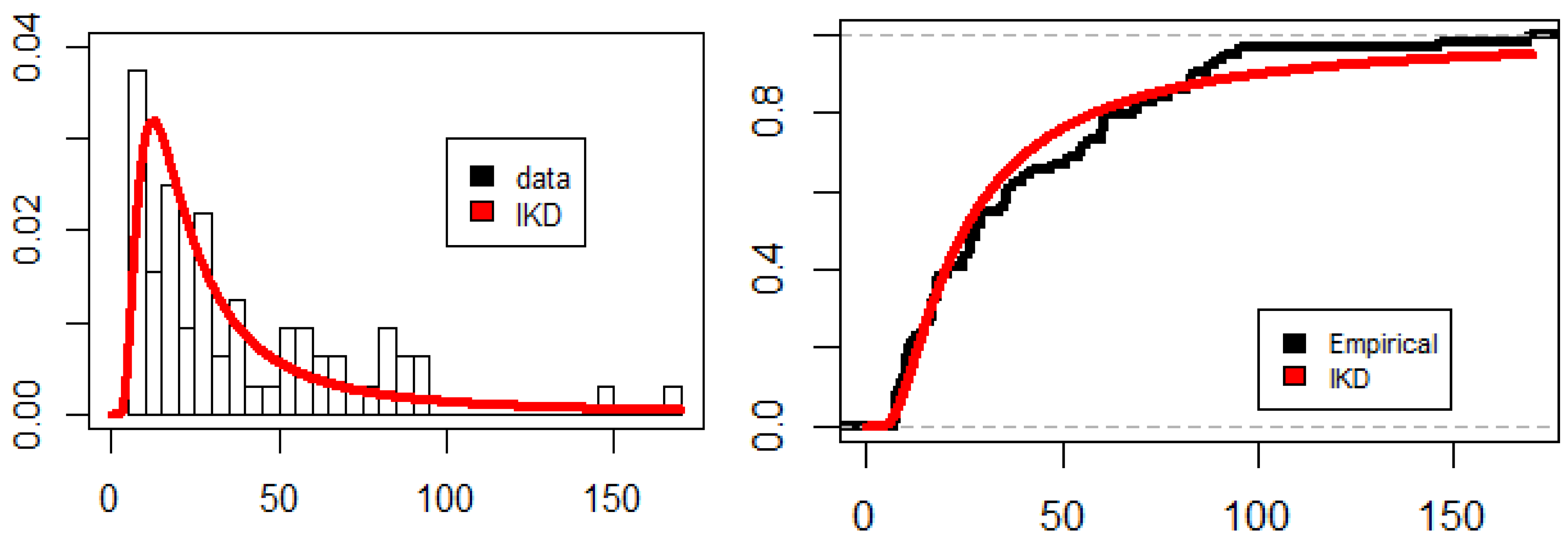
Using the Kolmogorov-Smirnov (K–S) test, the data set is checked for such a fitted model and the estimates are obtained using the ML method. With a p-value (PV) of 0.591, the K–S distance is 0.409. As a result, it is obvious that the IKD is a suitable model for fitting these data. Data’s estimated PDF and CDF are displayed in Figure 10. According to this graph, the IKD seems to be a suitable model for fitting the data.
Based on the aforementioned theoretical results, actual data sets are checked using the RSS and SRS sampling techniques. The SRS and RSS estimators from the IKD are shown in Table 13 and Table 14 for various set sizes under five and ten cycles utilizing different estimating techniques. The R-package is used to generate the RSS and SRS observations.
We considered the K–S test for quantifying the distance between the empirical distribution function of the real data and the CDF using the estimators’ parameters in each design, based on the choices of q and h, in order to demonstrate the superiority of RSS over the SRS using various estimation methods considered in this study. Be aware that we have substituted the K–S for the mean squared in this case. Obviously, estimators that outperform the other competitors have larger PVs (greater than 5%) and lower K–S values. Remember that for data, the MLEs based on SRS are regarded as the true population parameters.
The SRS design is considered for this dataset and for each estimation method, where the estimators are obtained using a sample of size qh = 40. Using the RSS with sample of sizes q = 4 and h = 10 is considered for calculating the estimators. We compare the SRS and RSS designs in terms of the K–S distance value and PVs results given in Table 15, and the corresponding fittings are displayed in Figure 11 and Figure 12. Due to the smallest values of the K–S and the corresponding largest PVs, the RSS is more efficient than the SRS based on the same number of measured units for all estimators.

7. Conclusions

This article considered the problem of RSS-based estimation for the IKD parameters using some estimation techniques; such as, the maximum likelihood, the maximum product of spacing, the ordinary and weighted least squares, the Cramer-von Mises, and the Anderson-Darling. With the aid of a simulation study and the use of a real dataset, the performance results of the proposed estimators are contrasted with those of their SRS equivalents based on the same number of measured units. The numerical simulation results show that for all outcomes shown in the tables with the same sample sizes, the proposed RSS estimators are superior to their SRS counterparts in terms of the smallest MSE. The estimates are asymptotically unbiased because their accuracy improves with sample size. The results of the real dataset also showed that the RSS design is superior to the SRS design due to the largest values for its P-values. As future research the IKD parameters can be estimated using other modifications of RSS as modified robust extreme ranked set sampling [32], neoteric RSS [33] and varied RSS [34]. Also, the process performance index of the IKD can be obtained in future [35,36].

Author Contributions

Conceptualization, A.S.H. and H.F.N.; methodology, A.S.H., A.I.A.-O., G.A.A. and H.F.N.; software A.S.H., A.I.A.-O. and H.F.N.; validation, A.S.H., A.I.A.-O., G.A.A. and H.F.N.; formal analysis, A.S.H., A.I.A.-O. and H.F.N.; resources, A.S.H. and H.F.N.; data curation, A.S.H., A.I.A.-O., G.A.A. and H.F.N.; writing—original draft preparation, A.S.H. and H.F.N.; writing—review and editing, A.S.H., A.I.A.-O., G.A.A. and H.F.N.; funding acquisition, G.A.A. All authors have read and agreed to the published version of the manuscript.

Funding

This research was funded by Princess Nourah bint Abdulrahman University Researchers Supporting Project number (PNURSP2022R226), Princess Nourah bint Abdulrahman University, Riyadh, Saudi Arabia.

Institutional Review Board Statement

Not applicable.

Informed Consent Statement

Not applicable.

Data Availability Statement

Datasets are available in the real data application section.

Acknowledgments

The authors thank the support from Princess Nourah bint Abdulrahman University Researchers Supporting Project number (PNURSP2022R226), Princess Nourah bint Abdulrahman University, Riyadh, Saudi Arabia. We thank the referees for their valuable suggestions which improved the paper.

Conflicts of Interest

The authors declare no conflict of interest.

References

  1. McIntyre, G.A. A method for unbiased selective sampling, using ranked sets. Aust. J. Agric. Res. 1952, 3, 385–390. [Google Scholar] [CrossRef]
  2. Takahasi, K.; Wakimoto, K. On unbiased estimates of the population mean based on the sample stratified by means of ordering. Ann. Inst. Stat. Math. 1968, 20, 1–31. [Google Scholar] [CrossRef]
  3. Stokes, S.L. Estimation of variance using judgment ordered ranked set samples. Biometrics 1980, 36, 35–42. [Google Scholar] [CrossRef]
  4. Lam, K.; Sinha, B.K.; Wu, Z. Estimation of parameters in a two-parameter exponential distribution using ranked set sample. Ann. Inst. Stat. Math. 1994, 46, 723–736. [Google Scholar] [CrossRef]
  5. Chuív, N.; Sinha, B.K.; Wu, Z. Estimation of location parameter of a Cauchy distribution using ranked set sample. Metr. Int. J. Theor. Appl. Stat. 1995, 42, 234–235. [Google Scholar] [CrossRef]
  6. Sinha, B.K.; Sinha, B.K.; Purkayastha, S. On some aspects of ranked set sampling for estimation of normal and exponential parameters. Stat. Risk Model. 1996, 14, 223–240. [Google Scholar] [CrossRef]
  7. Lam, K.; Sinha, B.K.; Wu, Z. Estimation of Location and Scale Parameters of a Logistic Distribution Using a Ranked Set Sample, In Statistical Theory and Applications: Papers in Honor of Herbert A. Davi; Nagaraja, H.N., Sen, P.K., Morrison, D.F., Eds.; Springer: New York, NY, USA, 1996; pp. 187–197. [Google Scholar]
  8. Bhoj, D.S.; Ahsanullah, M. Estimation of parameters of the generalized geometric distribution using ranked set sampling. Biometrics 1996, 52, 685–694. [Google Scholar] [CrossRef]
  9. Adatia, A. Estimation of parameters of the half-logistic distribution using generalized ranked set sampling. Comput. Stat. Data Anal. 2000, 33, 1–13. [Google Scholar]
  10. Abu-Dayyeh, W.A.; Al-Subh, S.A.; Muttlak, H.A. Logistic parameters estimation using simple random sampling and ranked set sampling data. Appl. Math. Comput. 2004, 150, 543–554. [Google Scholar] [CrossRef]
  11. Al-Hadhrami, S.A. Parametric estimation on modified Weibull distribution based on ranked set sampling. Eur. J. Sci. Res. 2010, 44, 73–78. [Google Scholar]
  12. Hassan, A.S. Maximum likelihood and Bayes estimators of the unknown parameters for exponentiated exponential distribution using ranked set sampling. Int. J. Eng. Res. Appl. 2013, 3, 720–725. [Google Scholar]
  13. Abu-Dayyeh, W.; Assrhani, A.; Ibrahim, K. Estimation of the shape and scale parameters of Pareto distribution using ranked set sampling. Stat. Pap. 2013, 54, 207–225. [Google Scholar]
  14. Dey, S.; Salehi, M.; Ahmadi, J. Rayleigh distribution revisited via ranked set sampling. Metron 2017, 75, 69–85. [Google Scholar]
  15. Esemen, M.; Gürler, S. Parameter estimation of generalized Rayleigh distribution based on ranked set sample. J. Stat. Comput. Simul. 2018, 88, 615–628. [Google Scholar] [CrossRef]
  16. Samuh, M.H.; Al-Omari, A.I.; Koyuncu, N. Estimation of the parameters of the new Weibull-Pareto distribution using ranked set sampling. Statistica 2020, 80, 103–123. [Google Scholar]
  17. Bantan, R.; Hassan, A.S.; Elsehetry, M. Zubair Lomax distribution: Properties and estimation based on ranked set sampling. CMC-Comput. Mater. Contin. 2020, 65, 2169–2187. [Google Scholar] [CrossRef]
  18. Al-Omari, A.I.; Benchiha, S.; Almanjahie, I.M. Efficient estimation of the generalized Quasi-Lindley distribution parameters under ranked set sampling and applications. Math. Probl. Eng. 2021, 2021, 9982397. [Google Scholar] [CrossRef]
  19. Pedroso, V.C.; Taconeli, C.A.; Giolo, S.R. Estimation based on ranked set sampling for the two-parameter Birnbaum–Saunders distribution. J. Stat. Comput. Simul. 2021, 91, 316–333. [Google Scholar] [CrossRef]
  20. He, X.-F.; Chen, W.-X.; Yang, R. Log-logistic parameters estimation using moving extremes ranked set sampling design. Appl. Math.-A J. Chin. Univ. 2021, 36, 99–113. [Google Scholar] [CrossRef]
  21. Taconeli, C.A.; Bonat, W.H. On the performance of estimation methods under ranked set sampling. Comput. Stat. 2020, 35, 1805–1826. [Google Scholar] [CrossRef]
  22. Al-Omari, A.I.; Benchiha, S.; Almanjahie, I.M. Efficient estimation of two-parameter Xgamma distribution parameters using ranked set sampling design. Mathematics 2022, 10, 3170. [Google Scholar] [CrossRef]
  23. Long, C.; Chen, W.; Yang, R.; Yao, D. Ratio estimation of the population mean using auxiliary information under the optimal sampling design. Probab. Eng. Inf. Sci. 2022, 36, 449–460. [Google Scholar] [CrossRef]
  24. Yousef, M.M.; Hassan, A.S.; Al-Nefaie, A.H.; Almetwally, E.M.; Almongy, H.M. Bayesian estimation using MCMC method of system reliability for inverted Topp–Leone distribution based on ranked set sampling. Mathematics 2022, 10, 3122. [Google Scholar] [CrossRef]
  25. Bantan, R.; Elsehetry, M.; Hassan, A.S.; Elgarhy, M.; Sharma, D.; Chesneau, C.; Jamal, F. A two-parameter model: Properties and estimation under ranked sampling. Mathematics 2021, 9, 1214. [Google Scholar] [CrossRef]
  26. Al-Omari, A.I.; Hassan, A.S.; Alotaibi, N.; Shrahili, M.; Nagy, H.F. Reliability estimation of inverse Lomax distribution using extreme ranked set sampling. Adv. Math. Phys. 2021, 2021. [Google Scholar] [CrossRef]
  27. Hassan, A.S.; Nagy, H.F. Reliability estimation in multicomponent stress-strength for generalized inverted exponential distribution based on ranked set sampling. GU J. Sci. 2022, 35, 314–331. [Google Scholar]
  28. Kumaraswamy, P. A generalized probability density function for double-bounded random processes. J. Hydrol. 1980, 46, 79–88. [Google Scholar] [CrossRef]
  29. Abd AL-Fattah, A.M.; El-Helbawy, A.A.; Al-Dayian, G.R. Inverted Kumaraswamy distribution: Properties and estimation. Pak. J. Stat. 2017, 33, 37–61. [Google Scholar]
  30. Cheng, R.; Amin, N. Maximum product of spacings estimation with application to the lognormal distribution. In Technical Report; Department of Mathematics, University of Wales: Cardiff, UK, 1979. [Google Scholar]
  31. Swain, J.J.; Venkatraman, S.; Wilson, J.R. Least-squares estimation of distribution functions in Johnson’s translation system. J. Stat. Comput. Simul. 1988, 29, 271–297. [Google Scholar] [CrossRef]
  32. Al-Omari, A.I. Estimation of mean based on modified robust extreme ranked set sampling. J. Stat. Comput. Simul. 2011, 81, 1055–1066. [Google Scholar] [CrossRef]
  33. Zamanzade, E.; Al-Omari, A.I. New ranked set sampling for estimating the population mean and variance. Hacet. J. Math. Stat. 2016, 45, 1891–1905. [Google Scholar] [CrossRef]
  34. Haq, A.; Brown, J.; Moltchanova, E.; Al-Omari, A.I. Varied L ranked set sampling scheme. J. Stat. Theory Pract. 2015, 9, 741–767. [Google Scholar] [CrossRef]
  35. Hassan, A.; Assar, S.; Selmy, A. Assessing the lifetime performance index of Burr Type III distribution under progressive Type II censoring. Pak. J. Stat. Oper. Res. 2021, 17, 633–647. [Google Scholar] [CrossRef]
  36. Zhu, J.; Xin, H.; Zheng, C.; Tsai, T.-R. Inference for the process performance index of products on the basis of power-normal distribution. Mathematics 2021, 10, 35. [Google Scholar] [CrossRef]
Figure 1. Plots of the IKD PDF for some parameters.
Mathematics 10 04102 g001
Figure 10. Estimated PDF and CDF Plots for IKD.
Mathematics 10 04102 g010
Figure 11. Plots of the estimated PDFs under SRS and RSS designs for the dataset for nº = qh = 40.
Mathematics 10 04102 g011
Figure 12. Plots of the estimated CDFs under SRS and RSS designs for the dataset for nº = qh = 40.
Mathematics 10 04102 g012
Table 1. MSE values for all parameter estimates of IKD under SRS.
n True
Value
MLMPSLSWLSCvMAD
PEMSEPEMSEPEMSEPEMSEPEMSEPEMSE
15 υ = 0.5 0.5850.1900.4610.0900.5140.1670.5290.1750.5890.2550.4370.107
τ = 0.8 1.0070.7280.7160.2990.8470.6330.8660.6161.0431.0580.7770.532
20 υ = 0.5 0.5640.1600.4660.0880.5050.1310.5210.1370.5710.1960.4530.102
τ = 0.8 0.9590.6210.7260.2980.8380.5880.8620.5570.9930.8850.7870.497
25 υ = 0.5 0.5450.1380.4640.0820.5060.1220.5170.1240.5560.1640.4720.104
τ = 0.8 0.9240.5040.7280.2600.8280.4320.8490.4320.9460.6080.8020.420
30 υ = 0.5 0.5430.1330.4720.0850.5110.1150.5180.1180.5490.1450.4720.102
τ = 0.8 0.9120.4660.7420.2590.8380.4180.8540.4300.9330.5570.7920.388
40 υ = 0.5 0.5300.1200.4740.0830.5060.1080.5130.1100.5340.1280.4700.096
τ = 0.8 0.8730.3810.7390.2330.8130.3400.8290.3440.8810.4250.7680.322
50 υ = 0.5 0.5270.1160.4790.0850.5120.1090.5160.1100.5340.1250.4740.099
τ = 0.8 0.8580.3520.7460.2300.8200.3300.8300.3310.8730.3960.7670.313
Table 2. MSE values for all parameter estimates of IKD under RRS.
qhTrue
Value
MLMPSLSWLSCvMAD
PEMSEPEMSEPEMSEPEMSEPEMSEPEMSE
35 υ = 0.5 0.5570.0290.4440.0200.4890.0370.4920.0300.5700.0700.5100.025
τ = 0.8 0.9360.1700.6700.1210.7720.2170.7850.1930.9640.3650.8240.153
10 υ = 0.5 0.5350.0080.4600.0100.4940.0150.5010.0140.5300.0200.5060.012
τ = 0.8 0.2260.3360.7090.0590.7890.0950.8050.0860.8770.1210.8180.071
45 υ = 0.5 0.5390.0160.4490.0150.4860.0250.4940.0260.5420.0380.5050.017
τ = 0.8 0.8920.0770.6800.0730.7660.1610.7860.1660.9000.2290.8090.079
10 υ = 0.5 0.5120.0040.4650.0070.4930.0100.4980.0080.5200.0120.5020.008
τ = 0.8 0.1880.3770.7130.0390.7760.0540.7890.0430.8410.0640.7990.041
55 υ = 0.5 0.5290.0010.4510.0100.4890.0140.4930.0120.5330.0200.5020.010
τ = 0.8 0.8620.0490.6840.0550.7620.0810.7750.0670.8680.1070.7980.053
10 υ = 0.5 0.4950.0030.4670.0050.4910.0060.4960.0050.5110.0070.4990.005
τ = 0.8 0.1670.4020.7230.0280.7740.0350.7870.0290.8250.0390.7960.027
Table 3. MSE values for all parameter estimates of IKD under SRS.
n True
Value
MLMPSLSWLSCvMAD
PEMSEPEMSEPEMSEPEMSEPEMSEPEMSE
15 υ = 0.5 0.5980.0620.4710.0290.5330.0650.5370.0620.6440.2920.5160.050
τ = 1.2 1.5370.7871.0950.3901.2810.7151.2920.6371.5961.2111.3100.704
20 υ = 0.5 0.5660.0310.4680.0180.5250.0410.5090.0240.5640.0420.5180.018
τ = 1.2 1.4190.3931.0780.2321.2460.4451.2050.2461.3970.4571.2440.206
25 υ = 0.5 0.5500.0230.4690.0150.5140.0270.5200.0240.5600.0390.5130.024
τ = 1.2 1.3790.2781.0900.1771.2410.3941.2640.3391.4110.5511.2600.283
30 υ = 0.5 0.5380.0190.4670.0140.5110.0240.5160.0190.5510.0310.5080.021
τ = 1.2 1.3330.1971.0830.1391.2290.2851.2740.2631.4010.3891.2660.249
40 υ = 0.5 0.5290.0120.4730.0090.5020.0140.5090.0120.5300.0170.5050.014
τ = 1.2 1.3060.1381.1060.1051.2110.1621.2340.1401.3120.1991.2310.148
50 υ = 0.5 0.5270.0100.4790.0080.5110.0120.5150.0100.5330.0140.5050.013
τ = 1.2 1.2900.1001.1200.0791.2340.1361.2470.1161.3150.1651.2290.131
Table 4. MSE values all parameter estimates of IKD under RSS.
qhTrue
Value
MLMPSLSWLSCvMAD
PEMSEPEMSEPEMSEPEMSEPEMSEPEMSE
35 υ = 0.5 0.5580.0320.4470.0220.4880.0340.4930.0320.5680.0590.5140.028
τ = 1.2 1.3900.3191.0030.2421.1440.4171.1610.3781.4320.7151.2370.321
10 υ = 0.5 0.5250.0110.4580.0100.4960.0160.4990.0130.5320.0200.5060.012
τ = 1.2 1.3080.1321.0710.1221.1870.1941.2060.1731.3210.2481.2310.141
45 υ = 0.5 0.5410.0180.4480.0140.4950.0250.4990.0220.5520.0380.5080.017
τ = 1.2 1.3560.1981.0270.1691.1790.2761.1750.2431.3840.3981.2390.200
10 υ = 0.5 0.5170.0070.4630.0070.4880.0100.4950.0080.5140.0120.4990.008
τ = 1.2 1.2540.0721.0680.0821.1450.1131.1720.0961.2400.1291.1890.084
55 υ = 0.5 0.5290.0100.4520.0100.4840.0130.4900.0110.5270.0180.5010.010
τ = 1.2 1.3090.1301.0370.1291.1440.1781.1680.1521.3010.2321.2090.142
10 υ = 0.5 0.5140.0040.4660.0050.4920.0060.4960.0050.5120.0060.4990.004
τ = 1.2 1.2470.0511.0810.0601.1620.0751.1800.0601.2380.0851.1900.055
Table 5. MSE values for all parameter estimates of IKD under SRS.
n True
Value
MLMPSLSWLSCvMAD
PEMSEPEMSEPEMSEPEMSEPEMSEPEMSE
15 υ = 1.5 1.9151.2041.3810.4451.6611.1381.6701.0292.1022.7101.7070.805
τ = 1.5 1.7390.3621.3560.2291.5420.4091.5560.3701.8030.6551.6010.300
20 υ = 1.5 1.7590.5281.3590.2511.5980.7101.6040.6181.8821.5041.6240.405
τ = 1.5 1.6520.2381.3490.1781.4980.2691.5150.2381.6780.3661.5490.207
25 υ = 1.5 1.7150.4431.3790.2341.6050.3721.6230.3331.8160.6311.6130.278
τ = 1.5 1.6150.1711.3610.1411.4950.1321.5210.1751.6340.2531.5360.156
30 υ = 1.5 1.7090.3411.4130.1891.5980.3721.6140.3391.7690.5611.6260.300
τ = 1.5 1.6290.1511.4020.1151.5360.1921.5540.1721.6540.2431.5670.149
40 υ = 1.5 1.6000.1711.3760.1241.5230.2271.5430.2031.6380.2971.5500.177
τ = 1.5 1.5670.0961.3870.0881.4910.1241.5120.1121.5760.1431.5220.101
50 υ = 1.5 1.5870.1271.3980.0971.5300.1721.5460.1501.6220.2181.5480.130
τ = 1.5 1.5630.0761.4100.0691.5080.1001.5250.0881.5770.1151.5300.078
Table 6. MSE values for all parameter estimates of IKD under RSS.
qhTrue
Value
MLMPSLSWLSCvMAD
PEMSEPEMSEPEMSEPEMSEPEMSEPEMSE
35 υ = 1.5 1.7790.6651.3020.3281.5190.9511.5290.8021.8801.9031.5930.660
τ = 1.5 1.6730.2481.3000.2021.4370.3261.4590.2891.6720.4501.5240.234
10 υ = 1.5 1.6520.1911.3810.1471.5270.2851.5500.2451.6860.4181.5760.222
τ = 1.5 1.5860.0941.3690.1001.4730.1391.4980.1211.5870.1651.5210.109
45 υ = 1.5 1.6900.3171.3150.2281.5000.4561.5250.4221.7500.7841.5580.323
τ = 1.5 1.6080.1421.3050.1561.4380.1981.4610.1781.6110.2511.5000.151
10 υ = 1.5 1.5820.1091.3640.0981.4930.1661.5040.1321.6060.2201.5210.120
τ = 1.5 1.5430.0571.3660.0701.4600.0881.4750.0711.5450.0991.4910.064
55 υ = 1.5 1.6100.1681.3100.1521.4550.2241.4780.2031.6390.3401.5130.179
τ = 1.5 1.5670.0971.3180.1191.4320.1301.4530.1211.5680.1541.4850.106
10 υ = 1.5 1.5570.0681.3750.0721.4740.1031.4940.0851.5610.1251.5050.074
τ = 1.5 1.5390.0411.3880.0531.4670.0641.4860.0531.5340.0691.4960.048
Table 7. MSE values for all parameter estimates of IKD under SRS.
n True
Value
MLMPSLSWLSCvMAD
PEMSEPEMSEPEMSEPEMSEPEMSEPEMSE
15 υ = 1.2 1.4940.6631.0980.2451.3371.171.3320.8221.652.2451.3450.476
τ = 0.8 0.9260.1140.7120.0720.8120.1330.8220.1170.9520.2030.8480.095
20 υ = 1.2 1.4690.3671.150.1561.3140.421.3250.371.5410.9061.3500.278
τ = 0.8 0.9280.0910.7520.0550.8280.0990.840.0880.9350.1460.8630.08
25 υ = 1.2 1.3590.2251.1090.1261.2520.2291.2610.2001.4060.3651.2810.189
τ = 0.8 0.8670.0580.7240.0460.8000.0630.8100.0560.880.0810.8230.052
30 υ = 1.2 1.3050.1591.0930.1041.2270.2251.2390.1791.3480.3171.2480.150
τ = 0.8 0.8460.0430.7220.0380.7930.0550.8040.0470.8590.0670.8130.042
40 υ = 1.2 1.2910.0941.1190.0661.2310.1241.2450.1081.3180.1661.2500.092
τ = 0.8 0.8420.0310.7400.0270.8010.0380.8110.0340.8490.0450.8160.031
50 υ = 1.2 1.2740.0791.1290.0591.2340.1061.2460.0931.3030.1341.2470.081
τ = 0.8 0.8370.0250.7510.0230.8070.0340.8170.03000.8460.0390.8190.027
Table 8. MSE values for all parameter estimates of IKD under RSS.
qhTrue
Value
MLMPSLSWLSCvMAD
PEMSEPEMSEPEMSEPEMSEPEMSEPEMSE
35 υ = 1.2 1.4220.3721.0560.1701.2240.4521.2250.3581.5141.0701.2720.259
τ = 0.8 0.8960.0770.6870.0620.7720.1030.7780.0830.9100.1550.8130.068
10 υ = 1.2 1.3040.1091.0990.0861.2180.1571.2380.1511.3350.2231.2520.126
τ = 0.8 0.8460.0340.7240.0370.7890.0480.8020.0460.8540.0580.8130.039
45 υ = 1.2 1.3350.1771.0590.1331.1780.2291.1970.2061.3580.3811.2340.175
τ = 0.8 0.8680.0480.7000.0470.7660.0650.7800.0590.8640.0830.8050.050
10 υ = 1.2 1.2570.0581.0940.0571.1900.0891.2050.0771.2750.1171.2140.064
τ = 0.8 0.8310.0190.7310.0230.7870.0290.7980.0250.8360.0340.8050.021
55 υ = 1.2 1.2890.0901.0580.0771.1530.1041.1680.0901.2870.1531.2030.078
τ = 0.8 0.8420.0280.7030.0320.7570.0370.7680.0310.8340.0440.7910.028
10 υ = 1.2 1.2330.0361.0950.0441.1850.0591.1950.0481.2500.0721.2010.042
τ = 0.8 0.8130.0130.7280.0180.7810.0200.7880.0160.8180.0220.7920.015
Table 9. Eff values for all estimates.
qhTrue ValueMLMPSLSWLSCvMAD
35 υ = 0.5 6.5524.5004.5145.8333.6434.280
τ = 0.8 4.2822.4712.9173.1922.8993.477
10 υ = 0.5 16.2208.5007.6678.4297.2508.500
τ = 0.8 1.3874.3904.4005.0004.6035.465
45 υ = 0.5 10.0005.8675.2405.2695.1586.000
τ = 0.8 8.0654.0823.6523.3553.8656.291
10 υ = 0.5 28.57111.69010.80013.25310.66712.468
τ = 0.8 1.0115.9746.2968.0006.6417.854
55 υ = 0.5 138.0008.2008.71410.3338.20010.722
τ = 0.8 10.2864.7275.3336.4485.6827.925
10 υ = 0.5 44.61517.00017.30221.19517.36120.625
τ = 0.8 0.8768.2149.42911.41410.15411.593
Table 10. Eff values for all estimates.
qhTrue ValueMLMPSLSWLSCvMAD
35 υ = 0.5 1.9381.3181.9121.9384.9491.786
τ = 1.2 2.4671.6121.7151.6851.6942.193
10 υ = 0.5 1.7271.4001.5001.4621.5501.750
τ = 1.2 1.4921.1391.4691.5201.5691.766
45 υ = 0.5 1.7221.2861.6401.0911.1051.059
τ = 1.2 1.9851.3731.6121.0121.1481.030
10 υ = 0.5 1.7391.2921.4001.3791.4171.842
τ = 1.2 1.9171.2801.4341.4581.5431.762
55 υ = 0.5 2.3001.5462.0772.1822.1672.400
τ = 1.2 2.1381.3722.2132.2302.3751.993
10 υ = 0.5 2.3101.5312.1432.1282.1883.023
τ = 1.2 1.9611.3171.8131.9331.9412.382
Table 11. Eff values for all estimates.
qhTrue ValueMLMPSLSWLSCvMAD
35 υ = 1.5 1.8111.3571.1971.2831.4241.220
τ = 1.5 1.4601.1341.2551.2801.4561.282
10 υ = 1.5 1.7851.2861.3051.3841.3421.351
τ = 1.5 1.6061.1501.3811.4211.4731.367
45 υ = 1.5 1.6661.1011.5571.4641.9181.254
τ = 1.5 1.6761.1411.3591.3371.4581.371
10 υ = 1.5 1.5691.2651.3671.5381.3501.475
τ = 1.5 1.6841.2571.4091.5771.4441.578
55 υ = 1.5 2.6371.5391.6611.6401.8561.553
τ = 1.5 1.7631.1851.0151.4461.6431.472
10 υ = 1.5 1.8681.3471.6701.7651.7441.757
τ = 1.5 1.8541.3021.5631.6601.6671.625
Table 12. Eff values for all estimates.
qhTrue ValueMLMPSLSWLSCvMAD
35 υ = 1.2 1.7821.4412.5882.2962.0981.838
τ = 0.8 1.4811.1611.2911.4101.3101.397
10 υ = 1.2 1.4591.2091.4331.1851.4221.190
τ = 0.8 1.2651.0271.1461.0221.1551.077
45 υ = 1.2 2.0731.1731.8341.7962.3781.589
τ = 0.8 1.8961.1701.5231.4921.7591.600
10 υ = 1.2 1.6211.1581.3931.4031.4191.438
τ = 0.8 1.6321.1741.3101.3601.3241.476
55 υ = 1.2 2.5001.6362.2022.2222.3862.423
τ = 0.8 2.0711.4381.7031.8061.8411.857
10 υ = 1.2 2.1941.3411.7971.9381.8611.929
τ = 0.8 1.9231.2781.7001.8751.7731.800
Table 13. SRS estimates of the data set based on different estimation methods.
n MLMPSLSWLSCvMAD
15 υ 52.75928.76622.74227.78632.43434.004
τ 1.291.1071.0241.0921.1271.147
20 υ 61.70737.744362.488566.907646.15149.261
τ 1.2321.0981.6231.7491.7711.146
25 υ 46.96731.39141.12947.97254.74238.924
τ 1.1961.0821.1231.1851.21.124
30 υ 89.659.69552.93867.71965.58166.906
τ 1.4261.3061.2491.3361.311.326
40 υ 65.61148.33587.959117.002109.63459.715
τ 1.2841.1981.3221.421.3811.237
Table 14. RSS estimates of the data set based on different estimation methods.
qh MLMPSLSWLSCvMAD
35 υ 30.9222.37813.25918.4717.11120.176
τ 1.1591.0590.8890.9960.9631.02
10 υ 40.77832.99319.16129.91222.27326.569
τ 1.2941.2281.0461.1921.0921.153
45 υ 49.99132.70923.52530.56829.3531.467
τ 1.2861.1671.0491.1381.1141.144
10 υ 64.69146.63746.46671.75753.78145.476
τ 1.3111.2281.1941.3541.2351.203
55 υ 56.25156.25143.07633.26644.66638.693
τ 1.331.331.261.1591.2721.204
Table 15. The PEs, KS and PV in SRS and RSS designs for the dataset at sample size for nº = qh = 40.
Method υ τ K–SPV
SRSRSSSRSRSSSRSRSSSRSRSS
ML65.61158.0351.2841.3650.1280.0960.5250.858
MPS48.33561.1981.1981.3820.1350.0980.4610.838
LS87.95938.4971.3221.2250.1400.1060.4110.761
WLS117.00252.3361.4201.3260.1140.0870.6740.924
CvM109.63444.2321.3811.2670.5910.0990.4090.826
AD59.71550.7931.2371.3160.1320.0890.4890.911
Publisher’s Note: MDPI stays neutral with regard to jurisdictional claims in published maps and institutional affiliations.

