Open AccessFeature PaperArticle Queueing Inventory System in Transport Problem by Khamis A. K. Al MaqbaliKhamis A. K. Al Maqbali SciProfiles Scilit Preprints.org Google Scholar 1,*,†, Varghese C. JoshuaVarghese C. Joshua SciProfiles Scilit Preprints.org Google Scholar 1,†, Ambily P. MathewAmbily P. Mathew SciProfiles Scilit Preprints.org Google Scholar 1,† and Achyutha KrishnamoorthyAchyutha Krishnamoorthy SciProfiles Scilit Preprints.org Google Scholar 1,2,† 1 Department of Mathematics, CMS College Kottayam, Kottayam 686001, Kerala, India 2 Department of Mathematics, Central University of Kerala, Chalingal 671316, Kerala, India * Author to whom correspondence should be addressed. † These authors contributed equally to this work. Mathematics 2023, 11(1), 225; https://doi.org/10.3390/math11010225 Submission received: 14 November 2022 / Revised: 19 December 2022 / Accepted: 26 December 2022 / Published: 2 January 2023 (This article belongs to the Special Issue Stochastic Modeling and Applied Probability, 2nd Edition) Download keyboard_arrow_down Download PDF Download PDF with Cover Download XML Download Epub Browse Figures Versions Notes Abstract: In this paper, we consider the batch arrival of customers to a transport station. Customers belonging to each category is considered as a single entity according to a BMMAP. An Erlang clock of order m starts ticking when the transport vessel reaches the station. When the Lth stage of the clock is reached, an order for the next vessel is placed. The lead time for arrival of the vessel follows exponential distribution. There are two types of rooms in this system: the waiting rooms and the service rooms for customers in the transport station and in the vessel, respectively. The waiting room capacity for customers of type 1 is infinite whereas those for customer of type 2 , … , k are of finite capacities. The service room capacity C j for customer type j , j = 1 , 2 , … , k is finite. Upon arrival, customers of category j occupy seats designated for that category in the vessel, provided there is at least one vacancy belonging to that category. The total number of vessels with the operator is h * . The service time of each vessel follows exponential distribution with parameter μ . Each group of customers belong to category j searches independently for customers of this category to mobilize passengers when the Erlang clock reaches L 1 where L 1 < L . The search time for customers of category j follows exponential distribution with parameter λ j . The stability condition is derived. Some performance measures are estimated. Keywords: batch marked markovian arrival process; batch arrival; Erlang clock; batch service; matrix analytic method MSC: 60K25; 60K30 1. IntroductionIn the literature on queueing inventory, there are some studies that have focused on queueing inventory in transport problems. Shajin et al. [1] studied a queueing-inventory problem in passenger transport system. In their study, there were two types of customers: high priority and low priority. High priority customers have a finite buffer to wait but low priority customers to wait have an finite capacity queue. The arrival of customers forms a marked Poisson process. Service time follows exponential distribution for each customer. Melikov and Molchanov [2] studied stock optimization in transportation/storage systems. Sigman and Simchi [3] studied light traffic heuristic for an M/G/1 queue with limited inventory. Neuts [4] introduced the general bulk service (GBS) rule: customers can be served in batches between the minimum and maximum batch sizes. Krishnamoorthy et al. [5] analyzed a queueing system with k stages of services. Customers can join a service from the beginning of any of the stages. The customer arrives at the first node according to MAP. At all other nodes, the customer arrives according to a distinct Poisson process. The service at each stage relies on the stage and the number of customers served in a batch. In their study, they gave some real examples in our life, such as elevators and transport systems. A public transport system serves customers from different locations in the city.Besides this, many studies have focused on transport systems based on queueing theory, such as [6,7,8,9]. In [8], the authors studied the optimization model of the buses number on the route based on queueing theory in a smart city.In the case of classical queues, Neuts and Ramalhoto [10] introduced the concept of search by server in their study. In the retrial queueing set up, the concept of search was introduced by Artalejo et.al [11]. This study has been extended to more general cases by D’Apice and Manzo [12], Sekar et al. [13], and Ayyappan and Udayageetha [14]. Sekar et al. [13] studied a single server retrial queueing system with orbit search under Erlang-K service. D’Apice and Manzo [12] studied a single server queueing system with search for customers in a finite capacity.In this paper, we consider the batch Marked Markovian arrival process (BMMAP) of customers to a transport station. Customers belonging to category j in each batch as a single entity and so even though there are j customers in the batch, we consider it as a single unit for our most of the purposes, where j = 1 , 2 , … , k . Customer category j arrives to the transport station according to batch Marked Markovian arrival process (BMMAP) with representation ( D 0 , D 1 , … , D k ) where the D j s ′ are each of order m 1 . There are two types of rooms in this system: the waiting rooms and the service rooms for customers type j are in the transport station and in the vessel, respectively. The waiting room capacity for category 1 customers is infinite, whereas those for category j customers are of finite capacities, which is denoted by W j , j = 2 , … , k . The service room capacity C j for category j customers j = 1 , 2 , … , k is finite. Category j customer batch, on arrival, occupies seats designated for that category in the vessel, provided that there is at least one of the required size vacancy belonging to that category; a vacant seat for category j means that there are j seats. We call such a “unit of seats” as one single entity.An Erlang clock of order m starts when a transport vessel reaches the station. The Erlang clock moves from phase m ′ to phase (m ′ + 1) with parameter ϕ . When the Erlang clock reaches the Lth phase, we place an order for the next vessel. The lead time for arrival of vessels follow exponential distribution with parameter θ . If the current vessel is in the transport station and a new vessel arrives to the station, the former leaves the station immediately. In the same time, an Erlang clock for the new vessel starts.The total number of vessels in this queueing inventory system is denoted by h * . The number of vessels, which are in operation to drop off passengers, is denoted by h . The service time of transport vessel follows exponential distribution with parameter μ . Each group of customers belonging to category j searches independently for customers of this category to mobilize passengers belonging to that category, provided there is vacancy. The search for customers starts only when the Erlang clock reaches L 1 where L 1 < L and service room for type j has customer type j less than C j . If the new arrival type j fills the last seat in this service room, then the search for this type of customers is terminated for the present vessel. The search time for category j customers follows exponential distribution with parameter λ j . If category 1 customers find that seats are not available in service room for this category, they must wait in the waiting room for category 1 (infinite capacity). Customers of category j ( j = 2 , 3 , … , k ) leave the system if their waiting room is full at the time of arrival of this category.The salient features of this paper are as follows:Transport problem with batch arrival of customers and reserved vessel of designated capacity for each category is presented and discussed for the first time.Search of customers to fill vacant seats belonging to each category, if any is done by customers belonging to that category only.An Erlang clock monitors the phase for starting search of customers for the current vehicle.The next vehicle is ordered when the Erlang clock reaches stage L, which requires an exponentially distributed amount of time to arrive at the station.The vehicle already present in the station leaves the moment given by min {realization of the Erlang clock, arrival of next vehicle, all seats are filled}.This paper is arranged as follows. Section 2 discusses the mathematical modeling of the problem under investigation. In Section 3, the stability of this system is investigated and the stationary system state distribution is computed. Performance measures are elaborated in Section 4. In Section 5, numerical investigation of the model is elaborated. Cost analysis is shown in Section 6. Finally, we summarize with a concluding Section 7. 2. Mathematical Description of the ModelFor the analysis of the model, we introduce the following notations: N j ( t ) : the number of category j customers in the waiting room for this category at time t where j = 1 , 2 , … , k . Y ( t ) : the phase of the arrival process. I j ( t ) : the number of category j customers in the service room for this category at time t where j = 1 , 2 , … , k . B ( t ) : the booking status for the transport vessel where B ( t ) = 1 If already order for a new vessel , 0 Not booking H ( t ) : the number of vessels which (in operation) leave the station on the way to drop off passengers at time t. G ( t ) : the phase of an Erlang clock of order m.The Erlang clock only starts when a transport vessel is available at station. γ ( t ) = 1 ( On ) If the transport vessel is available at a transport station , 0 ( Off ) If it is not available at a transport station . X ( t ) = { ( N 1 ( t ) , … , N k ( t ) , Y ( t ) , B ( t ) , H ( t ) , γ ( t ) , G ( t ) , I 1 ( t ) , … , I k ( t ) ) ; t ≥ 0 } is a continuous time Markov Chain on the state space. Therefore, this model can be studied as a level independent quasi-birth-death (LIQBD) process with state space is given by Ω = Ω 1 ∪ Ω 2 ∪ Ω 3 ∪ Ω 4 ∪ Ω 5 ∪ Ω 6 ∪ Ω 7 ; where Ω 1 = { ( n 1 , … , n k , y , b = 1 , h , γ = 0 ) : 0 ≤ n 1 ; 0 ≤ n j ≤ W j ; 1 ≤ y ≤ m 1 ; 0 ≤ h ≤ h * } ; Ω 2 = { ( 0 , … , 0 , y , b = 0 , h , γ = 1 , g , i 1 , … , i k ) : 1 ≤ y ≤ m 1 ; 0 ≤ h ≤ ( h * − 1 ) ; 1 ≤ g ≤ ( L − 1 ) ; 0 ≤ i j ≤ C j ∀ j ≠ j ′ ; i j ′ ≠ C j ′ ; j = 1 , 2 , … , k } ; Ω 3 = { ( 0 , … , 0 , y , b = 1 , h , γ = 1 , g , i 1 , … , i k ) : 1 ≤ y ≤ m 1 ; 0 ≤ h ≤ ( h * − 1 ) ; L ≤ g ≤ m ; 0 ≤ i j ≤ C j ∀ j ≠ j ′ ; i j ′ ≠ C j ′ ; j = 1 , 2 , … , k } ; Ω 4 = { ( 0 , n 2 , … , n k , y , b = 0 , h , γ = 1 , g , i 1 , … , i k ) : 1 ≤ y ≤ m 1 ; 0 ≤ n j ≤ W j ; j ≠ 1 ; 0 ≤ h ≤ ( h * − 1 ) ; 1 ≤ g ≤ ( L − 1 ) ; 0 ≤ i j ≤ C j ∀ j ≠ j ′ ; i j ′ ≠ C j ′ ; j = 1 , 2 , … , k } ; Ω 5 = { ( 0 , n 2 , … , n k , y , b = 1 , h , γ = 1 , g , i 1 , … , i k ) : 1 ≤ y ≤ m 1 ; 0 ≤ n j ≤ W j ; j ≠ 1 ; 0 ≤ h ≤ ( h * − 1 ) ; L ≤ g ≤ m ; 0 ≤ i j ≤ C j ∀ j ≠ j ′ ; i j ′ ≠ C j ′ ; j = 1 , 2 , … , k } ; Ω 6 = { ( n 1 , … , n k , y , b = 0 , h , γ = 1 , g , C 1 , … , i k ) : 1 ≤ y ≤ m 1 ; 1 ≤ n 1 ; 0 ≤ n j ≤ W j ; j ≠ 1 ; 0 ≤ h ≤ ( h * − 1 ) ; 1 ≤ g ≤ ( L − 1 ) ; 0 ≤ i j ≤ C j ∀ j ≠ j ′ ; i j ′ ≠ C j ′ ; j = 1 , 2 , … , k } ; Ω 7 = { ( n 1 , … , n k , y , b = 1 , h , γ = 1 , g , C 1 , … , i k ) : 1 ≤ y ≤ m 1 ; 1 ≤ n 1 ; 0 ≤ n j ≤ W j ; j ≠ 1 ; 0 ≤ h ≤ ( h * − 1 ) ; L ≤ g ≤ m ; 0 ≤ i j ≤ C j ∀ j ≠ j ′ ; i j ′ ≠ C j ′ ; j = 1 , 2 , … , k } ; With the following conditions (in case γ = 1 ):If 0 ≤ i j < C j then n j = 0 for j = 1 , 2 , … , k .If i 1 = C 1 then 0 ≤ n 1 .If i j = C j then 0 ≤ n j ≤ W j for j = 2 , 3 , … , k .If i j = C j ∀ j , then the Erlang clock expires.For category j customers, C j is the maximum capacity of their service room (in the vessel) where j = 1 , 2 , … , k , whereas W j is the maximum capacity of their waiting room (in the transport station) where j = 2 , 3 , … , k . Regarding the service rooms, the total number of individual seats is visualized in Figure 1 below.The terms of transitions of the states are given in Table 1, Table 2, Table 3, Table 4 and Table 5.The infinitesimal generator Q of the level independent quasi-birth-death (LIQBD) process with state space is of the form Q = B 00 B 01 B 10 A 1 A 0 A 2 A 1 A 0 A 2 A 1 A 0 ⋱ ⋱ ⋱ ; where B 00 = E 00 E 01 E 02 … E 0 ( k − 1 ) E 10 E 11 E 12 … E 1 ( k − 1 ) E 20 E 21 E 22 … E 2 ( k − 1 ) ⋮ ⋮ ⋮ … ⋮ E ( k − 1 ) 0 E ( k − 1 ) 1 E ( k − 1 ) 2 … E ( k − 1 ) ( k − 1 ) ; B 01 = E 0 ( k , 1 ) O … O E 1 ( k , 1 ) O … O E 2 ( k , 1 ) O … O ⋮ ⋮ ⋮ ⋮ E ( k − 1 ) ( k , 1 ) O … O B 10 = E ( k , 1 ) 0 O … O E ( k , 2 ) 0 O … O E ( k , 3 ) 0 O … O ⋮ ⋮ ⋮ ⋮ E ( k , C 1 ) 0 O … O A 1 = E 1 E 0 O … … … … O O E 1 E 0 O … … … O O O E 1 E 0 O … … O ⋮ ⋮ ⋱ ⋱ ⋱ ⋱ ⋱ O O O O … … … O E 1 ; A 2 = E 2 O O … … O O E 2 O O … O O O E 2 O … O ⋮ ⋮ ⋱ ⋱ ⋱ O O O O … … E 2 ; A 0 = O O O … … O O O O … … O O O O … … O ⋮ ⋮ ⋮ ⋮ ⋮ O E 0 O O … … O ; where all sub-matrices (the zero matrices, E 0 , E 1 and E 2 ) are matrices of same order.For example, we fix k = 3 , C 1 = 3 ; L 1 = 2 and L = 3 . We get the following matrices as in Appendix A. 3. Steady-State Analysis 3.1. Stability ConditionTheorem 1. The queueing inventory system generated by Q is stable if and only if π C 1 E 0 e * < ∑ i = 1 C 1 π i E 2 e * where π i is sub vector of order 1 × r * for i = 1 , 2 , … , C 1 . E 0 = ( I ( r * m 1 ) ⊗ D 1 ) where I ( r * m 1 ) is an identity matrix of order r * m 1 where r * m 1 is a positive integer number. e * is column vector of 1’s.Proof. Let A = A 2 + A 1 + A 0 . We can notice that A is an irreducible matrix. Thus, the stationary vector π of A exists such that π A = 0 π e = 1 . The Markov chain with the infinitesimal generator Q of the level independent quasi-birth-death (LIQBD) is stable if and only if π A 0 e < π A 2 e . Recall, A 0 is a square matrix and A 0 = O O O … … O O O O … … O O O O … … O ⋮ ⋮ ⋮ ⋮ ⋮ O E 0 O O … … O . E 0 = ( I ( r * m 1 ) ⊗ D 1 ) where I ( r * m 1 ) is an identity matrix of order r * m 1 where r * m 1 is a positive integer number. π A 0 e = ( π 1 , π 2 , π 2 , … , π C 1 ) A 0 e ; where π 1 , π 2 , … , π C 1 are sub vectors of order 1 × r * . π A 0 e = ( π C 1 E 0 , O , O , … , O ) e * e * ⋮ e * ; = π C 1 E 0 e * Recall that A 2 is a square matrix and A 2 = E 2 O O … … O O E 2 O O … O O O E 2 O … O ⋮ ⋮ ⋱ ⋱ ⋱ O O O O … … E 2 . π A 2 e = ( π 1 , π 2 , π 2 , … , π C 1 ) A 2 e ; where π 1 , π 2 , … , π C 1 are sub vectors of order 1 × r * . π A 2 e = ( π 1 E 2 , π 2 E 2 , π 3 E 2 , … , π C 1 E 2 ) e * e * ⋮ e * ; = π 1 E 2 e * + π 2 E 2 e * + ⋯ + π C 1 E 2 e * = ∑ i = 1 C 1 π i E 2 e * Then π A 2 e = ∑ i = 1 C 1 π i E 2 e * ; Since π A 0 e = π C 1 E 0 e * and π A 2 e = ∑ i = 1 C 1 π i E 2 e * then the queueing inventory system is stable if and only if π C 1 E 0 e * < ∑ i = 1 C 1 π i E 2 e * □ 3.2. Stationary DistributionThe stationary distribution of the Markov chain under consideration can obtained by solving the set of Equations (1) and (2). X Q = 0 ; (1) X e = 1 . (2) Let X be decomposed with Q as following: X = ( X 0 , X 1 , X 2 , … ) , where X r = ( Z C 1 r − C 1 + 1 , Z C 1 r − C 1 + 2 , … , Z C 1 r ) ; r = 1 , 2 , … where X 0 = ( X 00 , X 0 n k , X 0 n ( k − 1 ) , … , X 0 n 2 ) where X 00 = ( X 000 , X 0 i k , X 0 i ( k − 1 ) , … , X 0 i 2 , X 0 i 1 ) where X 000 = ( x 0 … 01 ( b = 1 ) h ( γ = 0 ) , x 0 … 02 ( b = 1 ) h ( γ = 0 ) , … , x 0 … 0 m 1 ( b = 1 ) h ( γ = 0 ) ) ; where h = 0 , 1 , 2 , … , h * ; X 0 i k = ( X 0 … 0 y ( b = 0 ) h ( γ = 1 ) g ′ 0 … 0 i k , X 0 … 0 y ( b = 1 ) h ( γ = 1 ) g ″ 0 … 0 i k ) ; where i k = 0 , 1 , 2 , … , C k ; y = 1 , 2 , … , m 1 ; h = 0 , 1 , 2 , … , ( h * − 1 ) ; g ′ = 1 , 2 , … , ( L − 1 ) ; g ″ = L , ( L + 1 ) , … , m ; X 0 i ( k − 1 ) = ( X 0 … 0 y ( b = 0 ) h ( γ = 1 ) g ′ 0 … 0 i ( k − 1 ) i k , X 0 … 0 y ( b = 1 ) h ( γ = 1 ) g ″ 0 … 0 i ( k − 1 ) i k ) ; where y = 1 , 2 , … , m 1 ; h = 0 , 1 , 2 , … , ( h * − 1 ) ; g ′ = 1 , 2 , … , ( L − 1 ) ; g ″ = L , ( L + 1 ) , … , m ; i k = 0 , 1 , 2 , … , C k ; i ( k − 1 ) = 1 , 2 , … , C ( k − 1 ) ; ⋮ X 0 i j = ( X 0 … 0 y ( b = 0 ) h ( γ = 1 ) g ′ 0 … i j … i k , X 0 … 0 y ( b = 1 ) h ( γ = 1 ) g ″ 0 … i j … i k ) ; where y = 1 , 2 , … , m 1 ; h = 0 , 1 , 2 , … , ( h * − 1 ) ; g ′ = 1 , 2 , … , ( L − 1 ) ; g ″ = L , ( L + 1 ) , … , m ; i k = 0 , 1 , 2 , … , C k ; i j = 1 , 2 , … , C j ; j = 1 , 2 , … , k ; ⋮ X 0 i 1 = ( X 0 … 0 y ( b = 0 ) h ( γ = 1 ) g ′ i 1 i 2 … i k , X 0 … 0 y ( b = 1 ) h ( γ = 1 ) g ″ i 1 i 2 … i k ) ; where y = 1 , 2 , … , m 1 ; h = 0 , 1 , 2 , … , ( h * − 1 ) ; g ′ = 1 , 2 , … , ( L − 1 ) ; g ″ = L , ( L + 1 ) , … , m ; i 1 = 1 , 2 , … , C 1 ; i j = 0 , 1 , 2 , … , C j ; j = 2 , 3 , … , k ; X 0 n k = ( X 00 n k , X 00 n k C k , X 00 n k i ( k − 1 ) C k , … , X 00 n k i 2 C k , X 00 n k i 1 C k ) where n k = 1 , 2 , … , W k ; X 00 n k = ( X 0 … n k 1 ( b = 1 ) h ( γ = 0 ) , X 0 … n k 2 ( b = 1 ) h ( γ = 0 ) , … , X 0 … n k m 1 ( b = 1 ) h ( γ = 0 ) ) ; where h = 0 , 1 , 2 , … , h * ; y = 1 , 2 , … , m 1 ; X 00 n k C k = ( X 00 n k y ( b = 0 ) h ( γ = 1 ) g ′ 0 … 0 C k , X 00 n k y ( b = 1 ) h ( γ = 1 ) g ″ 0 … 0 C k ) ; where n k = 1 , 2 , … , W k ; y = 1 , 2 , … , m 1 ; h = 0 , 1 , 2 , … , ( h * − 1 ) ; g ′ = 1 , 2 , … , ( L − 1 ) ; g ″ = L , ( L + 1 ) , … , m ; X 00 n k i ( k − 1 ) C k = ( X 00 n k y ( b = 0 ) h ( γ = 1 ) g ′ 0 … 0 i ( k − 1 ) C k , X 00 n k y ( b = 1 ) h ( γ = 1 ) g ″ 0 … 0 i ( k − 1 ) C k ) ; where n k = 1 , 2 , … , W k ; y = 1 , 2 , … , m 1 ; h = 0 , 1 , 2 , … , ( h * − 1 ) ; g ′ = 1 , 2 , … , ( L − 1 ) ; g ″ = L , ( L + 1 ) , … , m ; i ( k − 1 ) = 1 , 2 , … , C ( k − 1 ) ; ⋮ X 00 n k i 2 C k = ( X 00 n k y ( b = 0 ) h ( γ = 1 ) g ′ 0 i 2 i 3 … i ( k − 1 ) C k , X 00 n k y ( b = 1 ) h ( γ = 1 ) g ″ 0 i 2 i 3 … i ( k − 1 ) C k ) ; where i 2 = 1 , 2 , … , C 2 ; i j = 0 , 1 , 2 , … , C j ; j = 3 , 4 , … , k ; h = 0 , 1 , 2 , … , ( h * − 1 ) ; X 00 n k i 1 C k = ( X 00 n k y ( b = 0 ) h ( γ = 1 ) g ′ i 1 i 2 i 3 … i ( k − 1 ) C k , X 00 n k y ( b = 1 ) h ( γ = 1 ) g ″ i 1 i 2 i 3 … i ( k − 1 ) C k ) ; where i 2 = 1 , 2 , … , C 2 ; i j = 0 , 1 , 2 , … , C j ; j = 3 , 4 , … , k ; X 0 n ( k − 1 ) = ( X 00 n ( k − 1 ) , X 00 n ( k − 1 ) C ( k − 1 ) i k , X 00 n ( k − 1 ) i ( k − 2 ) C ( k − 1 ) , X 00 n ( k − 1 ) i ( k − 3 ) C ( k − 1 ) , … , X 00 n ( k − 1 ) i 2 C ( k − 1 ) , X 00 n ( k − 1 ) i 1 C ( k − 1 ) ) where n ( k − 1 ) = 1 , 2 , … , W ( k − 1 ) ; X 00 n ( k − 1 ) = ( X 0 … n ( k − 1 ) n k 1 ( b = 1 ) h ( γ = 0 ) , X 0 … n ( k − 1 ) n k 2 ( b = 1 ) h ( γ = 0 ) , … , X 0 … n ( k − 1 ) n k m 1 ( b = 1 ) h ( γ = 0 ) ) ; where h = 0 , 1 , 2 , … , h * ; y = 1 , 2 , … , m 1 ; n ( k − 1 ) = 1 , 2 , … , W k ; X 00 n ( k − 1 ) C ( k − 1 ) i k = ( X 0 … 0 n ( k − 1 ) n k y ( b = 0 ) h ( γ = 1 ) g ′ 0 … 0 C ( k − 1 ) i k , X 0 … 0 n ( k − 1 ) n k y ( b = 1 ) h ( γ = 1 ) g ″ 0 … 0 C ( k − 1 ) i k ) ; where n k = 0 , 1 , 2 , … , W k ; y = 1 , 2 , … , m 1 ; h = 0 , 1 , 2 , … , ( h * − 1 ) ; g ′ = 1 , 2 , … , ( L − 1 ) ; g ″ = L , ( L + 1 ) , … , m ; n ( k − 1 ) = 1 , 2 , … , W ( k − 1 ) ; ⋮ X 00 n ( k − 1 ) i 1 C ( k − 1 ) = ( X 0 … 0 n ( k − 1 ) n k y ( b = 0 ) h ( γ = 1 ) g ′ i 1 i 2 … C ( k − 1 ) i k , X 0 … 0 n ( k − 1 ) n k y ( b = 1 ) h ( γ = 1 ) g ″ i 1 i 2 … C ( k − 1 ) i k ) ; where n k = 0 , 1 , 2 , … , W k ; t y = 1 , 2 , … , m 1 ; h = 0 , 1 , 2 , … , ( h * − 1 ) ; g ′ = 1 , 2 , … , ( L − 1 ) ; g ″ = L , ( L + 1 ) , … , m ; n ( k − 1 ) = 1 , 2 , … , W ( k − 1 ) ; X 0 n 2 = ( X 00 n 2 , X 00 n 2 0 C 2 0 … 0 i k , X 00 n 2 0 C 2 0 … 0 i ( k − 1 ) i k , … , X 00 n 2 0 C 2 i 3 … i ( k − 1 ) i k ) ; where n 2 = 1 , 2 , … , W 2 ; X 00 n 2 = ( X 0 n 2 n 3 … n k 1 ( b = 1 ) h ( γ = 0 ) , X 0 n 2 n 3 … n k 2 ( b = 1 ) h ( γ = 0 ) , … , X 0 n 2 n 3 … n k m 1 ( b = 1 ) h ( γ = 0 ) ) ;where h = 0 , 1 , 2 , … , h * ; y = 1 , 2 , … , m 1 ; n 2 = 1 , 2 , … , W 2 ; X 00 n 2 i 1 C 2 00 i k = ( X 0 n 2 n 3 … n k y ( b = 0 ) h ( γ = 1 ) g ′ i 1 C 2 0 … 0 i k , X 0 n 2 n 3 … n k y ( b = 1 ) h ( γ = 1 ) g ″ i 1 C 2 0 … 0 i k ) ; where n 2 = 1 , 2 , … , W 2 ; y = 1 , 2 , … , m 1 ; h = 0 , 1 , 2 , … , ( h * − 1 ) ; g ′ = 1 , 2 , … , ( L − 1 ) ; g ″ = L , ( L + 1 ) , … , m ; ⋮ X 00 n 2 0 C 2 i 3 … i k = ( X 0 n 2 n 3 … n k y ( b = 0 ) h ( γ = 1 ) g ′ 0 C 2 i 3 … i k , X 0 n 2 n 3 … n k y ( b = 1 ) h ( γ = 1 ) g ″ 0 C 2 i 3 … i k ) ; where n 2 = 1 , 2 , … , W 2 ; y = 1 , 2 , … , m 1 ; h = 0 , 1 , 2 , … , ( h * − 1 ) ; g ′ = 1 , 2 , … , ( L − 1 ) ; g ″ = L , ( L + 1 ) , … , m ; Z n 1 = ( Z n 1 00 , Z n 1 0 , Z n 1 n k , Z n 1 n ( k − 1 ) , … , Z n 1 n 2 ) ; where 0 < n 1 ; Z n 1 00 = ( Z n 1 n 2 … n k 1 ( b = 1 ) h ( γ = 0 ) , Z n 1 n 2 … n k 2 ( b = 1 ) h ( γ = 0 ) , … , Z n 1 n 2 … n k m 1 ( b = 1 ) h ( γ = 0 ) ) ; where h = 0 , 1 , 2 , … , h * ; y = 1 , 2 , … , m 1 ; 0 < n 1 ; Z n 1 0 = ( Z n 1 0 … 0 y ( b = 0 ) h ( γ = 1 ) g ′ C 1 i 2 … i k , Z n 1 0 … 0 y ( b = 1 ) h ( γ = 1 ) g ″ C 1 i 2 … i k ) ; where h = 0 , 1 , 2 , … , ( h * − 1 ) ; y = 1 , 2 , … , m 1 ; Z n 1 n k = ( Z n 1 0 … n k y ( b = 0 ) h ( γ = 1 ) g ′ C 1 i 2 … C k , Z n 1 0 … n k y ( b = 1 ) h ( γ = 1 ) g ″ C 1 i 2 … C k ) ; where h = 0 , 1 , 2 , … , ( h * − 1 ) ; y = 1 , 2 , … , m 1 ; Z n 1 n ( k − 1 ) = ( Z n 1 0 … n ( k − 1 ) n k y ( b = 0 ) h ( γ = 1 ) g ′ C 1 i 2 … C ( k − 1 ) i k , Z n 1 0 … n ( k − 1 ) n k y ( b = 1 ) h ( γ = 1 ) g ″ C 1 i 2 … C ( k − 1 ) i k ) ; where h = 0 , 1 , 2 , … , ( h * − 1 ) ; y = 1 , 2 , … , m 1 ; ⋮ Z n 1 n 2 = ( Z n 1 n 2 … n k y ( b = 0 ) h ( γ = 1 ) g ′ C 1 C 2 i 3 … i k , Z n 1 n 2 … n k y ( b = 1 ) h ( γ = 1 ) g ″ C 1 C 2 i 3 … i k ) ; where h = 0 , 1 , 2 , … , ( h * − 1 ) ; y = 1 , 2 , … , m 1 ; n 2 = 1 , 2 , … , W k ; Note: in case ( γ = 1 ):If i j = C j ∀ j , then Erlang clock expires.If i j = C j , then 0 ≤ n j ≤ W j ; j = 2 , 3 , … , k .If i 1 = C 1 , then 0 ≤ n 1 .If i j < C j , then n j = 0 ; j = 1 , 2 , … , k . From Equation (1), we obtain the following equations. X 0 B 00 + X 1 B 10 = 0 ; (3) X 0 B 01 + X 1 A 1 + X 2 A 2 = 0 ; (4) X 1 A 0 + X 2 A 1 + X 3 A 2 = 0 ; (5) X j − 1 A 0 + X j A 1 + X j + 1 A 2 = 0 for j = 2 , 3 , … (6) Then there exists a matrix R such that X j = X 1 R ( j − 1 ) for j = 2 , 3 , … . For more details, we can see Stewart [15]. 4. Performance MeasuresWe obtain some performance measures of the system under steady state as following:Expected number of type 1 customers in the waiting room for type 1 E [ N 1 ] = ∑ n 1 = 1 ∞ n 1 Z n 1 e . Expected number of type j customers in waiting room type j for j = 2 , … , k . E [ N j ] = ∑ n j = 1 W j ∑ n ( j + 1 ) = 0 W ( j + 1 ) … ∑ n k = 0 W k ∑ y = 1 m 1 ∑ h = 0 h * n j X 0 n j n ( j + 1 ) … n k y ( b = 1 ) h ( γ = 0 ) e + ∑ n j = 1 W j ∑ n ( j + 1 ) = 0 W ( j + 1 ) … ∑ n k = 0 W k ∑ y = 1 m 1 ∑ h = 0 ( h * − 1 ) ∑ g ′ = 1 ( L − 1 ) ∑ i k = 0 C k n j X 0 n j n ( j + 1 ) … n k y ( b = 0 ) h ( γ = 1 ) g ′ 0 C j 0 … 0 i k e + ∑ n j = 1 W j ∑ n ( j + 1 ) = 0 W ( j + 1 ) … ∑ n k = 0 W k ∑ y = 1 m 1 ∑ h = 0 ( h * − 1 ) ∑ g ″ = L m ∑ i k = 0 C k n j X 0 n j n ( j + 1 ) … n k y ( b = 1 ) h ( γ = 1 ) g ″ 0 C j 0 … 0 i k e + … + ∑ n 2 = 1 W 2 ∑ n 3 = 0 W 3 … ∑ n k = 0 W k ∑ y = 1 m 1 ∑ h = 0 ( h * − 1 ) ∑ g ′ = 1 ( L − 1 ) ∑ i ( j − 1 ) = 0 C ( j − 1 ) ∑ i ( j + 1 ) = 0 C ( j + 1 ) … ∑ i k = 0 C k n j X 0 n 2 n 3 … n j … n k y ( b = 0 ) h ( γ = 1 ) g ′ 0 C 2 … i ( j − 1 ) C j i ( j + 1 ) … i k e + ∑ n 2 = 1 W 2 ∑ n 3 = 0 W 3 … ∑ n k = 0 W k ∑ y = 1 m 1 ∑ h = 0 ( h * − 1 ) ∑ g ″ = L m ∑ i ( j − 1 ) = 0 C ( j − 1 ) ∑ i ( j + 1 ) = 0 C ( j + 1 ) … ∑ i k = 0 C k n j X 0 n 2 n 3 … n k y ( b = 1 ) h ( γ = 1 ) g ″ 0 C 2 … i ( j − 1 ) C j i ( j + 1 ) … i k e + ∑ n 1 = 1 ∞ ∑ n 2 = 1 W 2 … ∑ n j = 1 W j ∑ n ( j + 1 ) = 0 W ( j + 1 ) … ∑ n k = 0 W k ∑ y = 1 m 1 ∑ h = 0 h * n j Z n 1 n 2 … n k y ( b = 1 ) h ( γ = 0 ) e + ∑ n 1 = 1 ∞ ∑ n 2 = 1 W 2 … ∑ n j = 1 W j ∑ n ( j + 1 ) = 0 W ( j + 1 ) … ∑ n k = 0 W k ∑ y = 1 m 1 ∑ h = 0 ( h * − 1 ) ∑ g ′ = 1 ( L − 1 ) ∑ i 3 = 0 C 3 … ∑ i k = 0 C k n j Z n 1 n 2 n 3 … n j … n k y ( b = 0 ) h ( γ = 1 ) g ′ C 1 C 2 i 3 … C j … i k e + ∑ n 1 = 1 ∞ ∑ n 2 = 1 W 2 … ∑ n j = 1 W j ∑ n ( j + 1 ) = 0 W ( j + 1 ) … ∑ n k = 0 W k ∑ y = 1 m 1 ∑ h = 0 ( h * − 1 ) ∑ g ″ = L m ∑ i 3 = 0 C 3 … ∑ i k = 0 C k n j Z n 1 n 2 n 3 … n j … n k y ( b = 1 ) h ( γ = 1 ) g ″ C 1 C 2 i 3 … C j … i k e Probability that the service room j is idle for j = 1 , 2 , … , k . b 1 0 = ∑ y = 1 m 1 ∑ h = 0 ( h * − 1 ) ∑ g ′ = 1 ( L − 1 ) ∑ i 1 = 0 C 1 … ∑ i ( j − 1 ) = 0 C ( j − 1 ) ∑ i ( j + 1 ) = 0 C ( j + 1 ) … ∑ i k = 0 C k X 0 … 0 y ( b = 0 ) h ( γ = 1 ) g ′ i 1 … ( i j = 0 ) … i k e + ∑ y = 1 m 1 ∑ h = 0 ( h * − 1 ) ∑ g ″ = L m ∑ i 1 = 0 C 1 … ∑ i ( j − 1 ) = 0 C ( j − 1 ) ∑ i ( j + 1 ) = 0 C ( j + 1 ) … ∑ i k = 0 C k X 0 … 0 y ( b = 1 ) h ( γ = 1 ) g ″ i 1 … ( i j = 0 ) … i k e + ∑ n 2 = 1 W 2 … ∑ n ( j − 1 ) = 0 W ( j − 1 ) ∑ n ( j + 1 ) = 0 W ( j + 1 ) … ∑ n k = 0 W k ∑ y = 1 m 1 ∑ h = 0 ( h * − 1 ) ∑ g ′ = 1 ( L − 1 ) ∑ i 1 = 0 C 1 … ∑ i ( j − 1 ) = 0 C ( j − 1 ) ∑ i ( j + 1 ) = 0 C ( j + 1 ) … ∑ i k = 0 C k X n 2 … n ( j − 1 ) n ( j + 1 ) … n k y ( b = 0 ) h ( γ = 1 ) g ′ i 1 … ( i j = 0 ) … i k e + ∑ n 2 = 1 W 2 … ∑ n ( j − 1 ) = 0 W ( j − 1 ) ∑ n ( j + 1 ) = 0 W ( j + 1 ) … ∑ n k = 0 W k ∑ y = 1 m 1 ∑ h = 0 ( h * − 1 ) ∑ g ″ = L m ∑ i 1 = 0 C 1 … ∑ i ( j − 1 ) = 0 C ( j − 1 ) ∑ i ( j + 1 ) = 0 C ( j + 1 ) … ∑ i k = 0 C k X n 2 … n ( j − 1 ) n ( j + 1 ) … n k y ( b = 1 ) h ( γ = 1 ) g ″ i 1 … ( i j = 0 ) … i k e + ∑ n 1 = 1 ∞ … ∑ n ( j − 1 ) = 0 W ( j − 1 ) ∑ n ( j + 1 ) = 0 W ( j + 1 ) … ∑ n k = 0 W k ∑ y = 1 m 1 ∑ h = 0 ( h * − 1 ) ∑ g ′ = 1 ( L − 1 ) ∑ i 1 = 0 C 1 … ∑ i ( j − 1 ) = 0 C ( j − 1 ) ∑ i ( j + 1 ) = 0 C ( j + 1 ) … ∑ i k = 0 C k Z n 1 n 2 … n ( j − 1 ) n ( j + 1 ) … n k y ( b = 0 ) h ( γ = 1 ) g ′ i 1 … ( i j = 0 ) … i k e + ∑ n 1 = 1 ∞ … ∑ n ( j − 1 ) = 0 W ( j − 1 ) ∑ n ( j + 1 ) = 0 W ( j + 1 ) … ∑ n k = 0 W k ∑ y = 1 m 1 ∑ h = 0 ( h * − 1 ) ∑ g ″ = L m ∑ i 1 = 0 C 1 … ∑ i ( j − 1 ) = 0 C ( j − 1 ) ∑ i ( j + 1 ) = 0 C ( j + 1 ) … ∑ i k = 0 C k Z n 1 n 2 … n ( j − 1 ) n ( j + 1 ) … n k y ( b = 1 ) h ( γ = 1 ) g ″ i 1 … ( i j = 0 ) … i k e Probability that the service room j is busy for j = 1 , 2 , … , k . b j 1 = 1 − b j 0 Expected number of vessels, which are in operation to drop off passengers. E [ N h ] = ∑ h = 0 h * ∑ y = 1 m 1 h x 0 … 0 y ( b = 1 ) h ( γ = 0 ) + ∑ h = 0 ( h * − 1 ) ∑ y = 1 m 1 ∑ g ′ = 1 ( L − 1 ) ∑ i k = 0 C k h X 0 … 0 y ( b = 0 ) h ( γ = 1 ) g ′ 0 … 0 i k e + ∑ h = 0 ( h * − 1 ) ∑ y = 1 m 1 ∑ g ″ = L m ∑ i k = 0 C k h X 0 … 0 y ( b = 1 ) h ( γ = 1 ) g ″ 0 … 0 i k e + ∑ h = 0 ( h * − 1 ) ∑ y = 1 m 1 ∑ g ′ = 1 ( L − 1 ) ∑ i ( k − 1 ) = 0 C ( k − 1 ) ∑ i k = 0 C k h X 0 … 0 y ( b = 0 ) h ( γ = 0 ) g ′ 0 … 0 i ( k − 1 ) i k e + ∑ h = 0 ( h * − 1 ) ∑ y = 1 m 1 ∑ g ″ = L m ∑ i ( k − 1 ) = 0 C ( k − 1 ) ∑ i k = 0 C k h X 0 … 0 y ( b = 1 ) h ( γ = 1 ) g ″ 0 … 0 i ( k − 1 ) i k e + … + ∑ h = 0 ( h * − 1 ) ∑ y = 1 m 1 ∑ g ′ = 1 ( L − 1 ) ∑ i 1 = 1 C 1 ∑ i 2 = 1 C 2 … ∑ i k = 0 C k h X 0 … 0 y ( b = 0 ) h ( γ = 1 ) g ′ i 1 i 2 … i k e + ∑ h = 0 ( h * − 1 ) ∑ y = 1 m 1 ∑ g ″ = L m ∑ i 1 = 1 C 1 ∑ i 2 = 1 C 2 … ∑ i k = 0 C k h X 0 … 0 y ( b = 1 ) h ( γ = 1 ) g ″ i 1 i 2 … i k e + ∑ h = 0 h * ∑ y = 1 m 1 h X 0 … n k y ( b = 1 ) h ( γ = 0 ) e + ∑ h = 0 ( h * − 1 ) ∑ y = 1 m 1 ∑ g ′ = 1 ( L − 1 ) h X 00 n k y ( b = 0 ) h ( γ = 1 ) g ′ 0 … 0 C k e + ∑ h = 0 ( h * − 1 ) ∑ y = 1 m 1 ∑ g ″ = L m h X 00 n k y ( b = 1 ) h ( γ = 1 ) g ″ 0 … 0 C k e + … + ∑ h = 0 ( h * − 1 ) ∑ y = 1 m 1 ∑ g ′ = 1 ( L − 1 ) ∑ i 3 = 1 C 3 ∑ i 4 = 1 C 4 … ∑ i k = 0 C k h X 0 n 2 n 3 … n k y ( b = 0 ) h ( γ = 1 ) g ′ 0 C 2 i 3 … i k e + ∑ h = 0 ( h * − 1 ) ∑ y = 1 m 1 ∑ g ″ = L m ∑ i 3 = 1 C 3 ∑ i 4 = 1 C 4 … ∑ i k = 0 C k h X 0 n 2 n 3 … n k y ( b = 1 ) h ( γ = 1 ) g ″ 0 C 2 i 3 … i k e + ∑ n 1 = 1 ∞ ∑ n 2 = 0 W 2 … ∑ n k = 0 W k ∑ y = 1 m 1 ∑ h = 0 h * h Z n 1 n 2 … n k y ( b = 1 ) h ( γ = 0 ) e + ∑ n 1 = 1 ∞ ∑ y = 1 m 1 ∑ h = 0 ( h * − 1 ) ∑ g ′ = 1 ( L − 1 ) ∑ i 2 = 0 C 2 ∑ i 3 = 0 C 3 … ∑ i k = 0 C k h Z n 1 0 … 0 y ( b = 0 ) h ( γ = 1 ) g ′ C 1 i 2 … i k e + ∑ n 1 = 1 ∞ ∑ y = 1 m 1 ∑ h = 0 ( h * − 1 ) ∑ g ′ = 1 ( L − 1 ) ∑ i 2 = 0 C 2 ∑ i 3 = 0 C 3 … ∑ i k = 0 C k h Z n 1 0 … 0 y ( b = 0 ) h ( γ = 1 ) g ′ C 1 i 2 … i k e + ∑ n 1 = 1 ∞ ∑ y = 1 m 1 ∑ h = 0 ( h * − 1 ) ∑ g ″ = L m ∑ i 2 = 0 C 2 ∑ i 3 = 0 C 3 … ∑ i k = 0 C k h Z n 1 0 … 0 y ( b = 1 ) h ( γ = 1 ) g ″ C 1 i 2 … i k e + ∑ n 1 = 1 ∞ ∑ n k = 1 W k ∑ y = 1 m 1 ∑ h = 0 ( h * − 1 ) ∑ g ′ = 1 ( L − 1 ) ∑ i 2 = 0 C 2 ∑ i 3 = 0 C 3 … ∑ i ( k − 1 ) = 0 C ( k − 1 ) h Z n 1 0 … n k y ( b = 0 ) h ( γ = 1 ) g ′ C 1 i 2 … C k e + ∑ n 1 = 1 ∞ ∑ n k = 1 W k ∑ y = 1 m 1 ∑ h = 0 ( h * − 1 ) ∑ g ″ = L m ∑ i 2 = 0 C 2 ∑ i 3 = 0 C 3 … ∑ i ( k − 1 ) = 0 C ( k − 1 ) h Z n 1 0 … n k y ( b = 1 ) h ( γ = 1 ) g ″ C 1 i 2 … C k e + … + ∑ n 1 = 1 ∞ ∑ n 2 = 1 W 2 … ∑ n k = 1 W k ∑ y = 1 m 1 ∑ h = 0 ( h * − 1 ) ∑ g ′ = 1 ( L − 1 ) ∑ i 3 = 0 C 3 … ∑ i k = 0 C k h Z n 1 n 2 … n k y ( b = 0 ) h ( γ = 1 ) g ′ C 1 C 2 i 3 … i k e + ∑ n 1 = 1 ∞ ∑ n 2 = 1 W 2 … ∑ n k = 1 W k ∑ y = 1 m 1 ∑ h = 0 ( h * − 1 ) ∑ g ″ = L m ∑ i 3 = 0 C 3 … ∑ i k = 0 C k h Z n 1 n 2 … n k y ( b = 1 ) h ( γ = 1 ) g ″ C 1 C 2 i 3 … i k e Expected number of type j customers in the service room type j for j = 1 , 2 , … , k E [ I j ] = ∑ y = 1 m 1 ∑ h = 0 ( h * − 1 ) ∑ g ′ = 1 ( L − 1 ) ∑ i 1 = 0 C 1 … ∑ i j = 0 C j … ∑ i k = 0 C k i j X 0 … 0 y ( b = 0 ) h ( γ = 1 ) g ′ i 1 … i j … i k e + ∑ y = 1 m 1 ∑ h = 0 ( h * − 1 ) ∑ g ″ = L m ∑ i 1 = 0 C 1 … ∑ i j = 0 C j … ∑ i k = 0 C k i j X 0 … 0 y ( b = 1 ) h ( γ = 1 ) g ″ i 1 … i j … i k e + ∑ n k = 1 W k ∑ y = 1 m 1 ∑ h = 0 ( h * − 1 ) ∑ g ′ = 1 ( L − 1 ) ∑ i 1 = 0 C 1 … ∑ i j = 0 C j … ∑ i k = 0 C k i j X 0 … 0 n k y ( b = 0 ) h ( γ = 1 ) g ′ i 1 … i j … C k e + ∑ n k = 1 W k ∑ y = 1 m 1 ∑ h = 0 ( h * − 1 ) ∑ g ″ = L m ∑ i 1 = 0 C 1 … ∑ i j = 0 C j … ∑ i k = 0 C k i j X 0 … 0 n k y ( b = 1 ) h ( γ = 1 ) g ″ i 1 … i j … C k e + … + ∑ n 2 = 1 W 2 … ∑ n j = 0 W j … ∑ n k = 1 W k ∑ y = 1 m 1 ∑ h = 0 ( h * − 1 ) ∑ g ′ = 1 ( L − 1 ) ∑ i 1 = 0 C 1 … ∑ i j = 0 C j … ∑ i k = 0 C k i j X 0 n 2 … n j … n k y ( b = 0 ) h ( γ = 1 ) g ′ i 1 … i j … i k e + ∑ n 2 = 1 W 2 … ∑ n j = 0 W j … ∑ n k = 1 W k ∑ y = 1 m 1 ∑ h = 0 ( h * − 1 ) ∑ g ″ = L m ∑ i 1 = 0 C 1 … ∑ i j = 0 C j … ∑ i k = 0 C k i j X 0 n 2 … n j … n k y ( b = 1 ) h ( γ = 1 ) g ″ i 1 … i j … i k e + ∑ n 1 = 1 ∞ ∑ n 2 = 1 W 2 … ∑ n j = 0 W j … ∑ n k = 1 W k ∑ y = 1 m 1 ∑ h = 0 ( h * − 1 ) ∑ g ′ = 1 ( L − 1 ) ∑ i 2 = 0 C 2 … ∑ i j = 0 C j … ∑ i k = 0 C k i j Z n 1 n 2 … n j … n k y ( b = 0 ) h ( γ = 1 ) g ′ C 1 i 2 … i j … i k e + ∑ n 1 = 1 ∞ ∑ n 2 = 1 W 2 … ∑ n j = 0 W j … ∑ n k = 1 W k ∑ y = 1 m 1 ∑ h = 0 ( h * − 1 ) ∑ g ″ = L m ∑ i 2 = 0 C 2 … ∑ i j = 0 C j … ∑ i k = 0 C k i j Z n 1 n 2 … n j … n k y ( b = 1 ) h ( γ = 1 ) g ″ C 1 i 2 … i j … i k e Expected number of seats filled in the vessel that just left. E [ P ] = ∑ j = 1 k j E [ I j ] Expected number of unoccupied seats in the vessel that just left. E [ U ] = ∑ j = 1 k j C j − ∑ j = 1 k j E [ I j ] 5. Numerical ExampleIn order to illustrate the performance measures of the system numerically, we fix k = 3 , C 1 = 3 , C 2 = 3 , C 3 = 3 , W 1 = 3 , W 2 = 3 , θ = 10 , h = 4 , λ 1 = 0.1 , λ 2 = 0.2 , λ 3 = 0.3 , μ = 5 , m = 4 , L 1 = 2 , L = 3 and ϕ = 3 . For (BMMAP) with representation ( D 0 , D 1 , D 2 , D 3 ) of order m 1 , we fix m 1 = 3 , D 0 = − 14.8 1 2 0.3 − 21.3 4 0.5 0 − 21.5 , D 1 = 0.3 5 0.5 1 2 3 1.2 1.5 2 , D 2 = 1 0.2 2 0.4 1.1 2.5 7 0.8 1 and D 3 = 0.3 0.5 2 3 1.5 2.5 1 3.5 3 . 5.1. The Effect of Parameter ϕ on Performance MeasuresTo analyse the effect of parameter ϕ on various performance measures, we use Table 6, Table 7, Table 8 and Table 9 and Figure 2, Figure 3 and Figure 4 as following:From Figure 2 and Figure 3, we can see that the expected number of type j customers in waiting room j decreases as ϕ increases where j = 1 , 2 , 3 . Moreover, we can see from Figure 4 that the probability that service room j is idle increases as ϕ increases where j = 1 , 2 , 3 . 5.2. The Effect of λ j on Performance Measures Where j = 1 , 2 , 3 To analyze the effect of parameter λ 1 on various performance measures, we use Table 10 and Figure 5, Figure 6 and Figure 7 as follows:From Figure 5, we can notice that the expected number of type 1 customers in waiting room 1 increases as λ 1 increases.However, from Figure 6, we can see that the expected number of type j customers in waiting room j decreases as λ 1 increases where j = 2 , 3 . Moreover, we can see from Figure 7 that the probability that service room 1 is busy increases as λ 1 increases but the probability that service room j , j = 2 , 3 is busy decreases as λ 1 increases.To study the effect of parameter λ 2 on various performance measures, we use Table 11 and Figure 8, Figure 9 and Figure 10 as following:From Figure 8, we can notice that the expected number of type 1 customers in the waiting room 1 decreases as λ 2 increases.We can notice from Figure 9 that the expected number of type 3 customers in the waiting room 3 decreases as λ 2 increases. However, the expected number of type 2 customers in the waiting room 2 increases when λ 2 increases.Moreover, we can see from Figure 10 that the probability that service room 2 is busy increases as λ 2 increases but the probability that service room j , j = 1 , 3 is busy decreases as λ 2 increases.From Table 12 and Figure 11, Figure 12 and Figure 13, we can notice the following:From Figure 11, we can notice that the expected number of type 1 customers in waiting room 3 decreases as λ 3 increases.We can notice from Figure 12 that the expected number of type 2 customers in waiting room 2 decreases as λ 3 increases. However, the expected number of type 3 customers in waiting room 3 increases when λ 3 increases.Moreover, we can see from Figure 13 that the probability that service room 3 is busy increases as λ 3 increases but the probability that service room j , j = 1 , 2 is busy decreases as λ 3 increases. 6. Cost AnalysisBased on the above performance measures, we define the expected total cost ( E T C ) per unit time as E T C = ∑ j = 1 k V 1 j E [ N j ] + ∑ j = 1 k V 2 j b j 0 * + V 3 E [ N h ] + V 4 E [ U ] (7) where E [ N j ] = Expected number of type j customers in waiting room j ; j = 1 , 2 , … k . E [ N h ] = Expected number of vessels, which are in operation to drop off passengers. E [ U ] = Expected number of unoccupied seats in the vessel that just left. b j 0 * = Fraction of time seats for type j customers remain unoccupied, where b j 0 * = b j 0 b j 0 + ( 1 − b j 1 ) ; j = 1 , 2 , … k . V 1 j = Holding cost/customer of type j/unit time in waiting room j; j = 1 , 2 , … k . V 2 j = Idle time cost of service room j; j = 1 , 2 , … k . . V 3 = Operating cost per vessel. V 4 = Cost per unoccupied seat.We fix k = 3 , V 11 = $ 10 ; V 12 = $ 15 ; V 13 = $ 20 ; V 21 = $ 3 ; V 22 = $ 6 ; V 23 = $ 9 ; V 3 = $ 50 and V 4 = $ 5 . Then, we compute E T C L = 3 and E T C L = 4 when L = 3 and L = 4 , as mentioned in Table 7 and Table 9, respectively. From Table 6, Table 7, Table 8 and Table 9 and Figure 14, we can realize that the optimal value of the expected total cost ( E T C L = 3 ) per unit time is E T C L = 3 = $ 96.9178 when ϕ = 6 and the optimal value of the expected total cost ( E T C L = 4 ) per unit time is E T C L = 4 = $ 98.5270 when ϕ = 8 for these two examples. 7. ConclusionsIn this paper we study the batch Marked Markovian arrival process (BMMAP) of customers to a transport station. Under steady state condition, various performance measures are estimated. We study the effect of parameter ϕ of Erlang distribution and search rate for customers on performance measures. Besides this, we compute the expected total cost per unit time. Author ContributionsConceptualization, K.A.K.A.M.; V.C.J.; A.P.M. and A.K; methodology, K.A.K.A.M.; V.C.J.; A.P.M. and A.K.; software, K.A.K.A.M.; V.C.J.; A.P.M. and A.K.; validation, K.A.K.A.M.; V.C.J.; A.P.M. and A.K.; formal analysis, K.A.K.A.M.; V.C.J.; A.P.M. and A.K.; investigation, K.A.K.A.M.; V.C.J.; A.P.M. and A.K.; resources, K.A.K.A.M.; V.C.J.; A.P.M. and A.K.; data curation, K.A.K.A.M.; V.C.J.; A.P.M. and A.K.; writing—original draft preparation, K.A.K.A.M.; V.C.J.; A.P.M. and A.K.; writing—review and editing, K.A.K.A.M.; V.C.J.; A.P.M. and A.K.; visualization, K.A.K.A.M.; V.C.J.; A.P.M. and A.K.; supervision, K.A.K.A.M.; V.C.J.; A.P.M. and A.K. All authors have read and agreed to the published version of the manuscript.FundingThe first author acknowledges the Indian Council for Cultural Relations (ICCR) (Order No: 2019-20/838) and Ministry of Higher Education, Research and Innovation, Order No: 2019/35 in Sultanate of Oman for their support.Institutional Review Board StatementNot applicable.Informed Consent StatementNot applicable.Data Availability StatementNot applicable.Conflicts of InterestThe authors declare no conflict of interest. Appendix AWe fix k = 3 , C 1 = 3 ; L 1 = 2 and L = 3 and we get the following matrices: Q = B 00 B 01 B 10 A 1 A 0 A 2 A 1 A 0 A 2 A 1 A 0 ⋱ ⋱ ⋱ ; where B 00 = E 00 E 01 E 02 E 10 E 11 E 12 E 20 O E 22 ; B 01 = E 03 O O E 13 O O E 23 O O ; B 10 = E 30 O O E 40 O O E 50 O O ; A 1 = E 33 E 34 O O E 33 E 34 O O E 33 ; A 0 = O O O O O O E 34 O O ; A 2 = E 63 O O O E 63 O O O E 63 ; where E 00 = S 00 Υ 01 O O … O Ψ 01 S 01 Υ 01 O … O O Ψ 02 S 02 Υ 01 O ⋮ ⋱ ⋱ ⋱ ⋮ O O O Ψ 0 ( h * − 1 ) S 0 ( h * − 1 ) Υ 02 O O O O Ψ 0 h * S 0 h * ; E 01 = Λ 01 O O … O O Λ 01 O … O ⋮ ⋱ ⋮ O O … O Λ 02 ; E 02 = Λ 03 O O … O O Λ 03 O … O ⋮ ⋱ ⋮ O O … O Λ 04 ; E 03 = Λ 05 O O … O O Λ 05 O … O ⋮ ⋱ ⋮ O O … O Λ 06 ; E 11 = S 10 Υ 11 O O … O Ψ 11 S 11 Υ 11 O … O O Ψ 12 S 12 Υ 11 O ⋮ ⋱ ⋱ ⋱ ⋮ O O O Ψ 1 ( h * − 1 ) S 1 ( h * − 1 ) Υ 12 O O O O Ψ 1 h * S 1 h * ; E 12 = Λ 11 O O … O O Λ 11 O … O ⋮ ⋱ ⋮ O O … O Λ 12 ; E 13 = Λ 13 O O … O O Λ 13 O … O ⋮ ⋱ ⋮ O O … O Λ 14 ; E 10 = Γ 10 δ 10 O O … O O Γ 10 δ 10 O … O ⋮ ⋱ ⋱ ⋮ O O … O Γ 11 O O O … O Γ 12 O ; E 22 = S 20 Υ 21 O O … O Ψ 21 S 21 Υ 21 O … O O Ψ 22 S 22 Υ 21 O ⋮ ⋱ ⋱ ⋱ ⋮ O O O Ψ 2 ( h * − 1 ) S 2 ( h * − 1 ) Υ 22 O O O O Ψ 2 h * S 2 h * ; E 20 = Γ 20 δ 20 O O … O O Γ 20 δ 20 O … O ⋮ ⋱ ⋱ ⋮ O O … O Γ 21 O O O … O Γ 22 O ; E 23 = Λ 21 O O … O O Λ 21 O … O ⋮ ⋱ ⋮ O O … O Λ 22 ; E 33 = S 30 Υ 31 O O … O Ψ 31 S 31 Υ 31 O … O O Ψ 32 S 32 Υ 31 O ⋮ ⋱ ⋱ ⋱ ⋮ O O O Ψ 3 ( h * − 1 ) S 3 ( h * − 1 ) Υ 32 O O O O Ψ 3 h * S 3 h * ; E 34 = Λ 31 O O … O O Λ 31 O … O ⋮ ⋱ ⋮ O O … O Λ 32 ; E 30 = Γ 30 δ 30 O O … O O Γ 30 δ 30 O … O ⋮ ⋱ ⋱ ⋮ O O … O Γ 31 O O O … O Γ 32 O ; E 40 = Γ 40 δ 40 O O … O O Γ 40 δ 40 O … O ⋮ ⋱ ⋱ ⋮ O O … O Γ 41 O O O … O Γ 42 O ; E 50 = Γ 50 δ 50 O O … O O Γ 50 δ 50 O … O ⋮ ⋱ ⋱ ⋮ O O … O Γ 51 O O O … O Γ 52 Γ 53 ; E 63 = Γ 60 δ 60 O O … O O Γ 60 δ 60 O … O ⋮ ⋱ ⋱ ⋮ O O … O Γ 61 O O O … O Γ 62 Γ 63 ; S 00 = γ 7 γ 8 O O O γ 27 γ 28 O O O γ 29 γ 28 O O O γ 29 where γ 7 = γ 0 γ 1 + γ 3 + γ 5 + γ 6 where γ 0 = D 0 − θ I ( m 1 ) θ I ( m 1 ) O ; γ 1 = O I ( ( C 3 + 1 ) ( C 2 + 1 ) ( C 1 + 1 ) − 1 ) ⊗ ( D 0 − ϕ I ( m 1 ) ) ; γ 2 = I ( C 3 ) ⊗ D 3 O O O ; γ 3 = O I ( ( C 2 + 1 ) ( C 1 + 1 ) − 1 ) ⊗ γ 2 O O O I ( C 3 − 1 ) ⊗ D 3 O O O ; γ 4 = I ( ( C 3 + 1 ) C 2 ) ⊗ D 2 O O O ; γ 5 = O I ( C 1 ) ⊗ γ 4 O O O I ( ( C 3 + 1 ) C 2 − 1 ) ⊗ D 2 O O O ; γ 6 = O I ( ( C 3 + 1 ) ( C 2 + 1 ) C 1 − 1 ) ⊗ D 1 O O γ 8 = O ϕ I ( ( C 3 + 1 ) ( C 2 + 1 ) ( C 1 + 1 ) m 1 − m 1 ) ; γ 27 = γ 26 + γ 11 + γ 16 + γ 18 + γ 19 + γ 20 + γ 21 where γ 26 = γ 22 + γ 23 + γ 24 + γ 25 ; γ 22 = I ( ( C 3 + 1 ) ( C 2 + 1 ) ( C 1 + 1 ) − 1 ) ⊗ ( D 0 − ϕ I ( m 1 ) ) ; γ 23 = O I ( ( C 2 + 1 ) ( C 1 + 1 ) − 1 ) ⊗ γ 2 O O O I ( C 3 − 1 ) ⊗ D 3 O O O ; γ 24 = O I ( C 1 ) ⊗ γ 4 O O O I ( ( C 3 + 1 ) C 2 − 1 ) ⊗ D 2 O O O ; γ 25 = O I ( ( C 3 + 1 ) ( C 2 + 1 ) C 1 − 1 ) ⊗ D 1 O O ; γ 11 = I ( ( C 2 + 1 ) ( C 1 + 1 ) − 1 ) ⊗ γ 10 O O O ; γ 10 = O [ 0 : ( C 3 − 2 ) ] T ⊗ λ 3 I ( m 1 ) O O ; γ 16 = ζ 1 [ 1 : ( C 2 − 2 ) ] T ⊗ ( I ( C 3 ) ⊗ λ 2 I ( m 1 ) ) ; ζ 1 = O I ( C 1 ) ⊗ γ 13 O ; γ 13 = O γ 12 O O O O ; γ 18 = O O O [ 1 : ( C 1 − 2 ) ] T ⊗ ( I ( ( C 3 + 1 ) ( C 2 + 1 ) − 1 ) ⊗ λ 1 I m 1 ) O O ; γ 19 = d i a g ( ( e 1 × ( ( C 2 + 1 ) ( C 1 + 1 ) − 1 ) ⊗ ( O , − λ 3 [ 1 : ( C 3 − 2 ) ] ⊗ e 1 × m 1 , O ) , O , ( − λ 3 [ 1 : ( C 3 − 2 ) ] ⊗ e 1 × m 1 ) , O ) ; γ 20 = d i a g ( ( O , − λ 2 [ 1 : ( C 2 − 2 ) ] ⊗ e 1 × ( C 3 + 1 ) m 1 , O ) , O , − λ 2 [ 1 : ( C 2 − 2 ) ] ⊗ e 1 × ( C 3 + 1 ) m 1 , O ) ; γ 21 = d i a g ( O , − λ 1 [ 1 : ( C 1 − 2 ) ] ⊗ e 1 × ( C 3 + 1 ) ( C 2 + 1 ) m 1 , O ) ; γ 28 = ϕ I ( ( C 3 + 1 ) ( C 2 + 1 ) ( C 1 + 1 ) m 1 − m 1 ) ; γ 29 = γ 27 − d i a g θ e 1 × ( C 3 + 1 ) ( C 2 + 1 ) ( C 1 + 1 ) m 1 − m 1 where S 0 h = S 00 − h μ d i a g ( e 1 × ( m 1 + ( ( C 3 + 1 ) ( C 2 + 1 ) ( C 1 + 1 ) m 1 − m 1 ) m ) ) where h = 1 , 2 , … , ( h * − 2 ) ; S 0 ( h * − 1 ) = S 00 − h μ d i a g ( e 1 × ( m 1 + ( ( C 3 + 1 ) ( C 2 + 1 ) ( C 1 + 1 ) m 1 − m 1 ) m ) ) + γ 48 ; S 0 h * = ( D 0 − h * μ I ( m 1 ) − θ I ( m 1 ) ) ; Ψ 0 h = h μ d i a g ( e 1 × ( m 1 + ( ( C 3 + 1 ) ( C 2 + 1 ) ( C 1 + 1 ) m 1 − m 1 ) m ) ) where h = 1 , 2 , … , ( h * − 1 ) ; Ψ 0 h * = h * μ I ( m 1 ) θ I ( m 1 ) O ; γ 48 = O O γ 35 O γ 35 O ; Υ 01 = γ 31 O γ 34 O γ 36 O γ 38 O where ; γ 31 = O O γ 30 O ; γ 30 = O D 1 O D 2 O D 3 ; γ 34 = γ 33 + γ 30 O where γ 33 = γ 32 O where γ 32 = O ( 1 : ( C 1 − 2 ) ) T ⊗ ζ 2 O ( 1 : ( C 2 − 2 ) ) T ⊗ ζ 3 O ( 1 : ( C 3 − 2 ) ) T ⊗ λ 3 I ( m 1 ) O ; ζ 2 = O λ 1 I ( m 1 ) ; ζ 3 = O λ 2 I ( m 1 ) ; γ 36 = γ 34 + γ 35 ; γ 35 = O e ( ( C 3 + 1 ) ( C 2 + 1 ) ( C 1 + 1 ) − 1 ) × 1 ⊗ ϕ I ( m 1 ) O ; γ 38 = γ 36 + γ 37 ; γ 37 = e ( ( C 3 + 1 ) ( C 2 + 1 ) ( C 1 + 1 ) − 1 ) × 1 ⊗ ϕ I ( m 1 ) O ; Υ 02 = O γ 30 γ 32 + γ 30 γ 32 + γ 30 ζ 4 ; ζ 4 = γ 32 + γ 30 + ( e ( ( C 3 + 1 ) ( C 2 + 1 ) ( C 1 + 1 ) − 1 ) × 1 ⊗ ϕ I ( m 1 ) ) ; Λ 01 = D 3 O O O I ( m ) ⊗ γ 40 O where ; γ 40 = I ( ( C 2 + 1 ) ( C 1 + 1 ) − 1 ) ⊗ ζ 5 O ; ζ 5 = O D 3 ; Λ 02 = D 3 O ; Λ 03 = D 2 O O O I ( m ) ⊗ γ 43 O ; γ 43 = I ( C 1 ) ⊗ ζ 6 O O O O I ( C 3 ) ⊗ D 2 ; ζ 6 = O ( I ( C 3 + 1 ) ⊗ D 2 ) ; Λ 04 = D 2 O ; Λ 05 = D 1 O O O O O γ 46 O ; γ 46 = I ( m ) ⊗ ζ 7 ; ζ 7 = O I ( ( C 3 + 1 ) ( C 2 + 1 ) − 1 ) ⊗ D 1 ; Λ 06 = D 1 O ; S 10 = γ 56 + γ 57 O O O O γ 83 + γ 85 ; γ 56 = I ( W 3 − 1 ) ⊗ ( − θ I ( m 1 ) + D 0 ) O O − θ I ( m 1 ) + D 0 + d i a g ( s u m ( D 3 , 2 ) ) T ; γ 57 = O I ( W 3 − 1 ) ⊗ D 3 O O ; γ 83 = γ 81 O O γ 82 ; γ 82 = γ 80 + ( I ( ( ( C 2 + 1 ) ( C 1 + 1 ) − 1 ) m ) ⊗ d i a g ( ( s u m ( D 3 , 2 ) ) T ) ) ; γ 81 = I ( W 3 − 1 ) ⊗ γ 80 ; γ 80 = γ 77 + γ 79 ; γ 77 = γ 63 O O O γ 74 O O O I ( m − 2 ) ⊗ γ 76 ; γ 63 = γ 60 + γ 61 + γ 62 ; γ 60 = O I ( C 1 ) ⊗ γ 59 O O O I ( C 2 − 1 ) ⊗ D 2 O O O ; γ 59 = I ( C 2 ) ⊗ D 2 O O O ; γ 61 = O I ( ( C 1 − 1 ) ( C 2 + 1 ) ) ⊗ D 1 O O O I ( C 2 ) ⊗ D 1 O O O ; γ 62 = ( I ( ( C 2 + 1 ) ( C 1 + 1 ) − 1 ) ⊗ ( D 0 − ϕ I ( m 1 ) ) ) ; γ 74 = γ 63 + γ 66 + γ 68 + γ 71 + γ 73 ; γ 66 = O I ( C 1 ) ⊗ γ 65 O O O O ; γ 65 = O O O O γ 64 O O O O ; γ 64 = ( [ 1 : ( C 2 − 2 ) ] T ⊗ λ 2 I ( m 1 ) ) ; γ 68 = O O O γ 67 O O where γ 67 = d i a g ( [ 1 : ( C 1 − 2 ) ] ⊗ ( e 1 × C 2 ⊗ λ 1 e 1 × m 1 ) ) ; γ 71 = d i a g ( ( e 1 × C 1 ⊗ γ 70 ) , O , γ 69 , O ) ; γ 70 = ( O , γ 69 , O ) ; γ 69 = ( [ 1 : ( C 2 − 2 ) ] ⊗ − λ 2 e 1 × m 1 ) ; γ 73 = d i a g ( [ O , γ 72 , O ] ) + d i a g ( [ O , ( [ 1 : ( C 1 − 2 ) ] ⊗ ( e 1 × C 2 ⊗ − λ 1 e 1 × m 1 ) ) , O , O ] ) γ 72 = ( [ 1 : ( C 1 − 2 ) ] ⊗ [ O 1 × C 2 m 1 , − λ 1 e 1 × m 1 ] ) ; γ 76 = γ 74 + γ 75 ; γ 75 = d i a g − θ e 1 × ( ( C 2 + 1 ) ( C 1 + 1 ) m 1 − m 1 ) ; γ 79 = O γ 78 O O ; γ 78 = I ( m − 1 ) ⊗ I ( ( C 2 + 1 ) ( C 1 + 1 ) − 1 ) ⊗ ϕ I ( m 1 ) ; γ 85 = O γ 84 O O ; γ 84 = I ( ( C 2 + 1 ) ( C 1 + 1 ) − 1 ) ( m ) ( W 3 − 1 ) ⊗ D 3 ; S 1 h = S 11 − h μ d i a g ( e 1 × ( W 3 m 1 + ( ( C 2 + 1 ) ( C 1 + 1 ) m 1 − m 1 ) m W 3 ) ) ; where h = 1 , 2 , … , ( h * − 1 ) ; S 1 h * = I ( W 3 − 1 ) ⊗ ( D 0 − θ I ( m 1 ) − h * μ I ( m 1 ) ) O O γ * + O I ( W 3 − 1 ) ⊗ D 3 O O where γ * = ( D 0 + d i a g ( ( s u m ( D 3 , 2 ) ) T ) − θ I ( m 1 ) − h * μ I ( m 1 ) ) ; Ψ 1 h = h μ d i a g ( e 1 × ( W 3 m 1 + ( ( C 2 + 1 ) ( C 1 + 1 ) m 1 − m 1 ) m W 3 ) ) where h = 1 , 2 , … , ( h * − 1 ) ; Ψ 1 h * = I ( W 3 ) ⊗ h * μ I ( m 1 ) O ; Υ 11 = O O γ 98 O where γ 98 = I ( W 3 ) ⊗ γ 97 where γ 97 = γ 92 + γ 94 + γ 96 where γ 96 = O e ( m − 1 ) × 1 ⊗ γ 95 where γ 95 = O 1 : ( C 1 − 2 ) T ⊗ ζ 8 O 1 : ( C 2 − 2 ) T ⊗ λ 2 I ( m 1 ) O ; ζ 8 = O λ 1 I ( m 1 ) ; γ 94 = O γ 93 where γ 93 = e ( ( C 2 + 1 ) ( C 1 + 1 ) − 1 ) × 1 ⊗ ϕ I ( m 1 ) ; γ 92 = e m × 1 ⊗ γ 91 ; γ 91 = O D 1 O D 2 ; Υ 12 = O γ 98 ; Λ 11 = O I ( W 3 ) ⊗ D 2 O O O O γ 102 O where γ 102 = I ( W 3 ) ⊗ I ( m ) ⊗ γ 101 ; γ 101 = I ( C 1 ) ⊗ ζ 9 O ; ζ 9 = O D 2 ; Λ 12 = O I ( W 3 ) ⊗ D 2 O ; Λ 13 = O I ( W 3 ) ⊗ D 1 O O O O O O γ 106 O where γ 106 = ( I ( W 3 ) ⊗ γ 105 ) ; γ 105 = I ( m ) ⊗ ζ 10 ; ζ 10 = O I ( C 2 ) ⊗ D 1 ; Λ 14 = O ( I ( W 3 ) ⊗ D 1 ) O ; Γ 10 = O I ( W 3 ) ⊗ θ I ( m 1 ) O O O O ; δ 10 = O O O O γ 89 O where γ 89 = I ( W 3 ) ⊗ ζ 11 ; ζ 11 = O e ( ( C 2 + 1 ) ( C 1 + 1 ) − 1 ) ( 2 ) × 1 ⊗ θ I ( m 1 ) ; Γ 11 = Γ 10 + δ 10 ; Γ 12 = O I ( W 3 ) ⊗ θ I ( m 1 ) O where S 20 = γ 175 + γ 125 ; γ 175 = γ 127 O O O O … O O γ 170 γ 173 O O … O O O γ 170 γ 173 O … O ⋮ ⋱ ⋱ ⋱ ⋱ ⋮ ⋮ O O … O γ 170 γ 173 O O O … O O γ 168 γ 169 where γ 127 = γ 120 + γ 121 + γ 122 + γ 119 ; γ 120 = I ( ( W 3 + 1 ) W 2 ) ⊗ ( D 0 − θ I ( m 1 ) ) ; γ 121 = d i a g ( e 1 × W 2 ⊗ ( O 1 × C 3 m 1 , ( s u m ( D 3 , 2 ) ) T ) ) ; γ 122 = d i a g ( O , ( e 1 × ( C 3 + 1 ) ⊗ ( s u m ( D 2 , 2 ) ) T ) ) ; γ 119 = γ 117 + γ 118 ; γ 117 = I ( W 2 ) ⊗ γ 116 ; γ 116 = O I ( W 3 ) ⊗ D 3 O O ; γ 118 = O I ( ( W 3 + 1 ) ( W 2 − 1 ) ) ⊗ D 2 O O ; γ 170 = γ 151 O O γ 165 where γ 151 = γ 134 γ 148 O O O γ 145 γ 148 O O O O γ 147 γ 148 O O ⋮ ⋮ ⋱ ⋱ ⋱ ⋱ ⋱ O … O O O γ 147 γ 148 O … O O O O γ 147 where γ 134 = γ 130 + γ 131 + γ 133 ; γ 130 = I ( C 1 ) ⊗ γ 129 O O O O ( I ( C 3 − 1 ) ⊗ D 3 ) O O O ; γ 131 = O I ( ( C 3 + 1 ) C 1 − 1 ) ⊗ D 1 O O ; γ 133 = I ( ( C 3 + 1 ) ( C 1 + 1 ) − 1 ) ⊗ γ 132 ; γ 132 = D 0 − ϕ I ( m 1 ) ; γ 145 = γ 134 + γ 137 + γ 140 + γ 142 + γ 144 ; γ 134 = γ 130 + γ 131 + γ 133 ; γ 137 = I ( C 1 ) ⊗ γ 136 O O O ; γ 136 = O γ 135 ; γ 135 = O 1 : ( C 3 − 2 ) ⊗ λ 3 I ( m 1 ) O ; γ 140 = d i a g ( e 1 × C 1 ⊗ γ 138 , γ 139 ) ; γ 139 = ( O , [ 1 : ( C 3 − 2 ) ] ⊗ − λ 3 e 1 × m 1 , O ) γ 138 = ( O , [ 1 : ( C 3 − 2 ) ] ⊗ − λ 3 e 1 × m 1 , O ) γ 142 = O O O γ 141 O O ; γ 141 = [ 1 : ( C 1 − 2 ) ] T ⊗ ζ 12 ; ζ 12 = I ( C 3 ) ⊗ λ 1 I ( m 1 ) O ; γ 144 = d i a g O 1 × ( C 3 + 1 ) m 1 γ 143 O ; γ 143 = [ 1 : ( C 1 − 2 ) ] ⊗ ( e 1 × ( C 3 + 1 ) ⊗ − λ 1 e 1 × m 1 ) ; γ 147 = γ 145 + γ 146 ; γ 146 = d i a g − θ e 1 × ( ( C 3 + 1 ) ( C 1 + 1 ) m 1 − m 1 ) ; γ 148 = ϕ I ( ( C 3 + 1 ) ( C 1 + 1 ) m 1 − m 1 ) ; γ 165 = γ 163 + γ 164 ; γ 163 = I ( W 3 − 1 ) ⊗ γ 160 O O O ; γ 160 = γ 153 + γ 154 + γ 159 ; γ 153 = I ( m ) ⊗ γ 152 ; γ 152 = O I ( C 3 − 1 ) ⊗ D 1 O O ; γ 154 = O I ( m − 1 ) ⊗ ( I ( C 3 ) ⊗ ϕ I ( m 1 ) ) O O ; γ 159 = γ 155 O O O γ 157 O O O I ( m − 2 ) ⊗ γ 158 ; γ 155 = I ( C 1 ) ⊗ ( D 0 − θ I ( m 1 ) ) ; γ 157 = γ 155 + γ 156 ; γ 156 = d i a g O [ 1 : ( C 1 − 2 ) ] ⊗ − λ 1 e 1 × m 1 O ; γ 158 = γ 157 + I ( C 1 ) ⊗ − θ I ( m 1 ) ; γ 162 = γ 160 + I ( C 1 m ) ⊗ d i a g ( ( s u m ( D 3 , 2 ) T ) ) ; γ 164 = O I ( W 3 − 1 ) ⊗ ( I ( C 1 m ) ⊗ D 3 ) O O ; γ 173 = γ 166 O O γ 167 ; γ 166 = I ( m ) ⊗ ( I ( ( C 3 + 1 ) ( C 1 + 1 ) − 1 ) ⊗ D 2 ) ; γ 167 = I ( W 3 ) ⊗ ( I ( C 1 m ) ⊗ D 2 ) ; γ 168 = γ 151 + I ( ( ( C 3 + 1 ) ( C 1 + 1 ) − 1 ) m ) ⊗ d i a g ( ( s u m ( D 2 , 2 ) T ) ) ; γ 169 = γ 165 + I ( C 1 m W 3 ) ⊗ d i a g ( ( s u m ( D 2 , 2 ) T ) ) ; γ 125 = O O O γ 124 ; γ 124 = I ( W 2 ) ⊗ O γ 123 O γ 123 where γ 123 = I ( m ) ⊗ ζ 13 O ; ζ 13 = I ( C 1 ) ⊗ ζ 14 O ; ζ 14 = O D 3 ; S 2 h = S 20 − h μ d i a g ( e 1 × ( ( W 3 + 1 ) W 2 m 1 + ( ( ( C 3 + 1 ) ( C 1 + 1 ) m 1 − m 1 ) m + ( ( C 1 + 1 ) m 1 − m 1 ) m W 3 ) W 2 ) ) where h = 1 , 2 , … , ( h * − 1 ) ; S 2 h * = γ 119 + γ 206 ; γ 206 = γ 204 O O γ 205 ; γ 204 = I ( W 2 − 1 ) ⊗ γ 203 ; γ 203 = I ( W 3 ) ⊗ γ 201 O O γ 202 ; γ 201 = D 0 − h * μ I ( m 1 ) − θ I ( m 1 ) ; γ 202 = D 0 − h * μ I ( m 1 ) − θ I ( m 1 ) + d i a g ( s u m ( D 3 , 2 ) T ) ; γ 205 = γ 203 + ( I ( W 3 + 1 ) ⊗ d i a g ( s u m ( D 2 , 2 ) T ) ) ; Ψ 2 h = h μ d i a g ( e 1 × ( ( W 3 + 1 ) W 2 m 1 + ( ( ( C 3 + 1 ) ( C 1 + 1 ) m 1 − m 1 ) m + ( ( C 1 + 1 ) m 1 − m 1 ) m W 3 ) W 2 ) ) where h = 1 , 2 , … , ( h * − 1 ) ; Ψ 2 h * = I ( ( W 3 + 1 ) W 2 ) ⊗ h * μ I ( m 1 ) O ; Υ 21 = O O γ 196 O where γ 196 = I ( W 2 ) ⊗ γ 188 O O γ 195 ; γ 195 = I ( W 2 ) ⊗ ζ * ; ζ * = γ 189 γ 192 γ 192 e ( m − 3 ) × 1 ⊗ γ 194 ; γ 194 = γ 193 + γ 192 ; γ 192 = γ 191 + γ 189 ; γ 191 = O γ 190 O ; γ 189 = O D 1 ; γ 193 = ( e C 3 × 1 ⊗ ϕ I ( m 1 ) ) ; γ 188 = γ 182 γ 186 γ 186 ζ 15 ; ζ 15 = e ( m − 3 ) × 1 ⊗ ( γ 187 + γ 186 ) O ; γ 187 = e ( ( C 3 + 1 ) ( C 1 + 1 ) − 1 ) × 1 ⊗ ϕ I ( m 1 ) ; γ 186 = γ 182 + γ 185 ; γ 185 = O γ 183 O γ 184 O ; γ 182 = O D 1 O D 3 ; Υ 22 = O γ 196 ; Λ 21 = O I ( W 3 + 1 ) W 2 ⊗ D 1 O O O O O I ( W ( 2 ) ) ⊗ γ 199 where γ 199 = I ( m ) ⊗ ζ 16 O ; ζ 16 = O I ( C 3 ) ⊗ D 1 ; Λ 22 = O I ( W 3 + 1 ) W 2 ⊗ D 1 ; Γ 20 = O I ( W 3 + 1 ) W 2 ) ⊗ I ( m 1 ) O O O O ; Γ 21 = γ 176 + δ 20 ; δ 20 = O O O O I ( W 2 ) ⊗ ζ 17 O ; ζ 17 = γ 178 γ 180 ; γ 178 = O O γ 177 O ; γ 177 = e ( C 3 + 1 ) ( C 1 + 1 ) ( m − 2 ) × 1 ⊗ θ I ( m 1 ) ; γ 180 = O I ( W 3 ) ⊗ ζ 18 ; ζ 18 = O γ 179 ; γ 179 = e C 1 ( m − 2 ) × 1 ⊗ θ I ( m 1 ) ; Γ 22 = O I ( W 2 ) ⊗ ( I ( W 3 + 1 ) ⊗ θ I ( m 1 ) ) O ; S 30 = γ 226 O O O O γ 244 γ 270 γ 272 O O γ 257 O O O O γ 268 ; γ 226 = γ 220 + γ 222 + γ 225 ; γ 225 = I ( W 2 ) ⊗ γ 223 O O ( γ 223 + γ 224 ) ; γ 224 = I ( W 3 + 1 ) ⊗ d i a g ( s u m ( D 2 , 2 ) T ) ; γ 223 = I ( W 3 ) ⊗ ( D 0 − θ I ( m 1 ) ) O O ( D 0 − θ I ( m 1 ) ) ⊗ d i a g ( s u m ( D 3 , 2 ) T ) ) ; γ 222 = O γ 221 O O ; γ 221 = I ( ( W 3 + 1 ) W 2 ) ⊗ D 2 ; γ 220 = I ( ( W 2 + 1 ) ) ⊗ γ 219 ; γ 219 = O I ( W 3 ) ⊗ D 3 O O ; γ 244 = γ 242 + γ 243 ; γ 243 = O I ( m − 1 ) ⊗ ϕ I ( ( C 3 + 1 ) ( C 2 + 1 ) m 1 − m 1 ) O O ; γ 242 = γ 231 O O O γ 240 O O O I ( m − 2 ) ⊗ γ 241 ; γ 241 = γ 240 − θ I ( ( C 3 + 1 ) ( C 2 + 1 ) m 1 − m 1 ) ; γ 240 = γ 231 + γ 234 + γ 236 + γ 238 + γ 239 ; γ 239 = d i a g ( O , [ 1 : ( C 2 − 2 ) ] ⊗ ( e 1 × ( C 3 + 1 ) ⊗ − λ 2 e 1 × m 1 ) , O ) ; γ 238 = d i a g ( ( e 1 × W 2 ⊗ γ 237 ) , O , ( [ 1 : ( C 3 − 2 ) ] ⊗ − λ 3 e 1 × m 1 ) , O ) ; γ 236 = O O O γ 235 O O ; γ 235 = [ 1 : ( C 2 − 2 ) ] T ⊗ ζ 19 ; ζ 19 = I ( C 3 ) ⊗ λ 2 I ( m 1 ) O ; γ 234 = I ( C 2 ) ⊗ γ 233 O O O ; γ 233 = O γ 232 ; γ 232 = O 1 : ( C 3 − 2 ) T ⊗ λ 3 I ( m 1 ) O ; γ 231 = γ 230 + γ 229 + ( I ( ( C 3 + 1 ) ( C 2 + 1 ) − 1 ) ⊗ D 0 ) − ϕ I ( ( C 3 + 1 ) ( C 2 + 1 ) m 1 − m 1 ) ; γ 230 = O I ( ( C 3 + 1 ) C 2 − 1 ) ⊗ D 2 O O ; γ 229 = I ( C 2 ) ⊗ γ 227 O O γ 228 ; γ 228 = O I ( C 3 − 1 ) ⊗ D 3 O O ; γ 257 = γ 255 + γ 256 ; γ 256 = O I ( W 3 − 1 ) ⊗ ( I ( m ) ⊗ ( I ( C 2 ) ⊗ D 3 ) ) O O ; γ 255 = I ( W 3 − 1 ) ⊗ γ 253 O O γ 254 ; γ 253 = γ 251 + γ 252 ; γ 252 = O ϕ I ( C 2 m 1 ( m − 1 ) ) O O ; γ 251 = γ 247 O O O γ 249 O O O I ( m − 2 ) ⊗ γ 250 ; γ 250 = γ 249 − I ( C 2 ) ⊗ θ I ( m 1 ) ; γ 249 = γ 247 + γ 248 ; γ 248 = d i a g ( [ O , ( 1 : ( C 2 − 2 ) ⊗ − λ 2 e 1 × m 1 ) , O ] ) ; γ 247 = γ 245 + γ 246 ; γ 246 = I ( C 2 ) ⊗ ( D 0 − ϕ I ( m 1 ) ) ; γ 245 = O I ( C 2 − 1 ) ⊗ D 2 O O ; γ 254 = γ 253 + I ( C 2 m ) ⊗ d i a g ( ( s u m ( D 3 , 2 ) ) T ) ; γ 268 = I ( W 2 − 1 ) ⊗ γ 265 O O ( γ 265 + γ 266 ) + γ 267 where γ 267 = O I ( W 2 − 1 ) ⊗ ( I ( m ) ⊗ ( I ( 3 ) ⊗ D 2 ) ) O O ; γ 266 = I ( m ) ⊗ ( I ( C 3 ) ⊗ d i a g ( ( s u m ( D 2 , 2 ) ) T ) ) ; γ 265 = γ 263 + γ 264 ; γ 264 = O I ( m − 1 ) ⊗ ( I ( C 3 ) ⊗ ϕ I ( m 1 ) ) O O ; γ 263 = γ 259 O O O γ 261 O O O I ( m − 2 ) ⊗ γ 262 ; γ 259 = γ 258 + I ( C 3 ) ⊗ ( D 0 − ϕ I ( m 1 ) ) ; γ 258 = O I ( C 3 − 1 ) ⊗ D 3 O O ; γ 262 = γ 261 + I ( C 3 ) ⊗ − θ I ( m 1 ) ; γ 261 = γ 259 + γ 260 ; γ 260 = d i a g ( [ O , ( 1 : ( C 3 − 2 ) ⊗ − λ 3 e 1 × m 1 ) , O ] ) ; γ 270 = γ 269 O ; γ 269 = I ( m ) ⊗ ζ 20 ; ζ 20 = I ( W 2 ) ⊗ ζ 21 O ; ζ 21 = O D 3 ; γ 272 = γ 271 O ; γ 271 = I ( m ) ⊗ ζ 22 ; ζ 22 = O I ( C 3 ) ⊗ D 2 ; S 3 h = S 30 − h μ d i a g ( e 1 × ( ( W 3 + 1 ) ( W 2 + 1 ) m 1 + ( ( C 3 + 1 ) ( C 2 + 1 ) m 1 − m 1 ) m + C 2 m 1 m W 3 + C 3 m 1 m W 2 ) ) where h = 1 , 2 , … , ( h * − 1 ) ; S 3 h * = γ 306 + γ 307 + γ 313 ; γ 313 = γ 311 + γ 312 ; γ 312 = ( I ( W 3 + 1 ) ( W 2 + 1 ) ⊗ ( − h * μ I ( m 1 ) − θ I ( m 1 ) ) ) ; γ 311 = γ 309 O O γ 310 ; γ 310 = γ 308 + ( I ( W 3 + 1 ) ⊗ d i a g ( s u m ( D 2 , 2 ) T ) ) γ 308 = I ( C 3 ) ⊗ D 0 O O D 0 + d i a g ( s u m ( D 3 , 2 ) T ) ; γ 309 = I ( W 2 ) ⊗ γ 308 ; Ψ 3 h = h μ d i a g ( e 1 × ( ( W 3 + 1 ) ( W 2 + 1 ) m 1 + ( ( C 3 + 1 ) ( C 2 + 1 ) m 1 − m 1 ) m + C 2 m 1 m W 3 + C 3 m 1 m W 2 ) ) where h = 1 , 2 , … , ( h * − 1 ) ; Ψ 3 h * = I ( ( W 3 + 1 ) ( W 2 + 1 ) ) ⊗ h * μ I ( m 1 ) O ; Υ 31 = O O γ 279 O γ 286 O γ 293 O ; γ 293 = O I ( W 2 ) ⊗ γ 292 ; γ 292 = γ 287 O γ 289 O γ 289 O e ( m − 3 ) × 1 ⊗ γ 291 O ; γ 291 = γ 289 + γ 290 ; γ 290 = e C 3 × 1 ⊗ ϕ I ( m 1 ) ; γ 289 = γ 287 + γ 288 ; γ 288 = O 1 : ( C 2 − 2 ) T ⊗ λ 3 I ( m 1 ) O ; γ 287 = O D 3 ; γ 286 = O I ( W 3 ) ⊗ γ 285 O ; γ 285 = γ 280 γ 282 γ 282 e ( m − 3 ) × 1 ⊗ γ 284 ; γ 284 = γ 282 + γ 283 ; γ 283 = e C 2 × 1 ⊗ ϕ I m 1 ; γ 282 = γ 280 + γ 281 ; γ 281 = O 1 : ( C 2 − 2 ) T ⊗ λ 2 I ( m 1 ) O ; γ 280 = O D 2 ; Υ 32 = O γ 279 γ 286 γ 293 ; γ 279 = γ 274 O γ 276 O γ 276 O e ( m − 3 ) × 1 ⊗ γ 278 O ; γ 278 = γ 276 + γ 277 ; γ 277 = e ( ( C 3 + 1 ) ( C 2 + 1 ) − 1 ) × 1 ⊗ ϕ I m 1 ; γ 276 = γ 274 + γ 275 ; γ 275 = O 1 : ( C 2 − 2 ) T ⊗ ζ 23 O 1 : ( C 3 − 2 ) T ⊗ λ 3 I ( m 1 ) O ; ζ 23 = O λ 2 I ( m 1 ) ; γ 274 = O D 2 O D 3 ; Γ 30 = O I ( ( W 3 + 1 ) ( W 2 + 1 ) ) ⊗ θ I ( m 1 ) O O O O ; Γ 31 = γ 296 + δ 30 ; δ 30 = O O O O O O γ 297 O O O O O γ 299 O O O O O γ 301 O ; γ 297 = e ( ( C 3 + 1 ) ( C 2 + 1 ) − 1 ) ( m − 2 ) × 1 ⊗ θ I ( m 1 ) ; γ 299 = I ( W 3 ) ⊗ ζ 24 ; ζ 24 = O γ 298 ; γ 298 = e C 2 ( m − 2 ) × 1 ⊗ θ I ( m 1 ) ; γ 301 = I ( W 2 ) ⊗ ζ 25 ; ζ 25 = O γ 300 ; γ 300 = e C 3 ( m − 2 ) × 1 ⊗ θ I ( m 1 ) O ; Γ 32 = O I ( ( W 3 + 1 ) ( W 2 + 1 ) ) ⊗ θ I ( m 1 ) O ; Λ 31 = D 1 I ( ( W 3 + 1 ) ( W 2 + 1 ) + ( ( C 3 + 1 ) ( C 2 + 1 ) − 1 ) m + C 2 m W 3 + C 3 m W 2 ) ; Λ 32 = I ( ( W 3 + 1 ) ( W 2 + 1 ) ) ⊗ D 1 ; Γ 40 = O I ( ( W 3 + 1 ) ( W 2 + 1 ) ) ⊗ θ I ( m 1 ) O O O O ; δ 40 = O O O O γ 331 O ; γ 331 = γ 326 γ 328 γ 330 ; γ 330 = O I ( W 2 ) ⊗ γ 329 ; γ 329 = O O e C 3 ( m − 2 ) × 1 ⊗ θ I ( m 1 ) O ; γ 328 = O γ 327 O ; γ 327 = I ( W 3 ) ⊗ ζ 26 ; ζ 26 = O e C 2 ( m − 2 ) × 1 ⊗ θ I ( m 1 ) ; γ 326 = O O e ( ( C 3 + 1 ) ( C 2 + 1 ) − 1 ) ( m − 2 ) ) × 1 ⊗ θ I ( m 1 ) O ; Γ 41 = γ 325 + γ 332 ; Γ 42 = O I ( ( W 3 + 1 ) ( W 2 + 1 ) ) ⊗ θ I ( m 1 ) O ; Γ 50 = O γ 339 O O O O ; γ 339 = I ( ( W 3 + 1 ) ( W 2 + 1 ) − 1 ) ⊗ θ I ( m 1 ) O ; δ 50 = O O O O θ I ( m 1 ) O O O O O γ 342 O O O γ 343 O O O γ 344 O O O γ 345 O ; γ 345 = O O O O e C 3 ( m − 2 ) × 1 ⊗ θ I ( m 1 ) O ; γ 344 = O I ( W 2 − 1 ) ⊗ γ 329 O ; γ 343 = O γ 327 O ; γ 342 = O O e ( ( C 3 + 1 ) ( C 2 + 1 ) − 1 ) ( m − 2 ) × 1 ⊗ θ I ( m 1 ) O ; Γ 52 = O I ( ( W 3 + 1 ) ( W 2 + 1 ) − 1 ) ⊗ θ I ( m 1 ) O O O O ; Γ 53 = O θ I ( m 1 ) ; Γ 60 = γ 353 O ; γ 353 = O I ( ( W 3 + 1 ) ( W 2 + 1 ) − 1 ) ⊗ θ I ( m 1 ) O O O O ; δ 60 = O O O O θ I ( m 1 ) O O O O O γ 342 O O O γ 343 O O O γ 344 O O O γ 345 O ; Γ 61 = Γ 60 + δ 60 ; Γ 17 = O I ( ( W 3 + 1 ) ( W 2 + 1 ) − 1 ) ⊗ θ I ( m 1 ) O O O O ; Γ 63 = O O θ I ( m 1 ) O ; ReferencesShajin, D.; Jacob, J.; Vishnevskiy, V.M.; Krishnamoorthy, A. On a Queueing-Inventory Problem in Passenger Transport System. In Distributed Computer and Communication Networks; DCCN 2019, Communications in Computer and Information Science; Vishnevskiy, V., Samouylov, K., Kozyrev, D., Eds.; Springer: Cham, Switzerland, 2019; Volume 1141, pp. 215–229. [Google Scholar]Melikov, A.Z.; Molchanov, A.A. Stock optimization in transportation/storage systems. Cybern. Syst. Anal. 1992, 28, 484–487. [Google Scholar] [CrossRef]Sigman, K.; Simchi-Levi, D. Light traffic heuristic for an M/G/1 queue with limited inventory. Ann. Oper. Res. 1992, 40, 371–380. [Google Scholar] [CrossRef]Neuts, M.F. A general class of bulk queues with Poisson input. Ann. Math. Stat. 1967, 38, 759–770. [Google Scholar] [CrossRef]Krishnamoorthy, A.; Joshua, A.N.; Vishnevsky, V. Analysis of a k-Stage Bulk Service Queuing System with Accessible Batches for Service. Mathematics 2021, 9, 559. [Google Scholar] [CrossRef]Jacyna, M.; Żak, J.; Gołębiowski, P. The Use of the Queueing Theory for the Analysis of Transport Processes. Logist. Transp. 2019, 41, 101–111. [Google Scholar] [CrossRef]Radmilovic, Z.; Colic, V.; Hrle, Z. Some aspects of storage and bulk queueing systems in transport operations. Transp. Plan. Technol. 1996, 20, 67–81. [Google Scholar] [CrossRef]Podlesna, L.; Bublyk, M.; Grybyk, I.; Matseliukh, Y.; Burov, Y.; Kravets, P.; Lozynska, O.; Karpov, I.; Peleshchak, I.; Peleshchak, R. Optimization Model of the Buses Number on the Route Based on Queueing Theory in a Smart City. In Proceedings of the MoMLeT+ DS, Lviv, Ukraine, 2–3 June 2020; pp. 502–515. [Google Scholar]Corkindale, D.R. Queueing Theory in the Solution of a Transport Evaluation Problem. J. Oper. Res. Soc. 1975, 26, 259–271. [Google Scholar] [CrossRef]Neuts, M.F.; Ramalhoto, M.F. A service model in which the server is required to search for customers. J. Appl. Probab. 1984, 21, 157–166. [Google Scholar] [CrossRef]Artalejo, J.R.; Joshua, V.C.; Krishnamoorthy, A. An M/G/1 Retrial Queue with Orbital Search by Server. In Advances in Stochastic Modelling; Notable Publications: NJ, USA, 2002; pp. 41–54. [Google Scholar]D’Apice, C.; Manzo, R. Search for customers in a finite capacity queueing system with phase-type distributions. Inf. Process. Electron. Sci. J. 2003, 3, 61–69. [Google Scholar]Sekar, G.; Ayyappan, G.; Subdramanian, A.M.G. Single Server Retrial Queueing System with Orbital search under Erlang K Service. Int. J. Appl. Math. 2012, 3, 454–463. [Google Scholar]Ayyappan, G.; Udayageetha, J. Transient analysis of M [X1], M [X2]/G1, G2/1 retrial queueing system with priority services, collisions, orbital search, working breakdown, start up/close down time, feedback, modified Bernoulli vacation and balking. Int. J. Appl. Eng. Res. 2018, 13, 8783–8795. [Google Scholar]Stewart, W.J. Probability, Markov Chains, Queues, and Simulation: The Mathematical Basis of Performance Modeling; Princeton University Press: Princeton, NJ, USA, 2009. [Google Scholar] Figure 1. The total number of individual seats in a specific service room. Figure 1. The total number of individual seats in a specific service room. Figure 2. Effect of ϕ on expected number of type 1 customers in waiting room 1. Figure 2. Effect of ϕ on expected number of type 1 customers in waiting room 1. Figure 3. Effect of ϕ on expected number of customers in the waiting room. Figure 3. Effect of ϕ on expected number of customers in the waiting room. Figure 4. Effect of ϕ on probability that the service room is idle. Figure 4. Effect of ϕ on probability that the service room is idle. Figure 5. Effect of λ 1 on expected number of type 1 customers in waiting room 1. Figure 5. Effect of λ 1 on expected number of type 1 customers in waiting room 1. Figure 6. Effect of λ 1 on expected number of type 2 , 3 customers in waiting room 2 , 3 . Figure 6. Effect of λ 1 on expected number of type 2 , 3 customers in waiting room 2 , 3 . Figure 7. Effect of λ 1 on probability that the service room is idle. Figure 7. Effect of λ 1 on probability that the service room is idle. Figure 8. Effect of λ 2 on expected number of type 1 customers in the waiting room 1. Figure 8. Effect of λ 2 on expected number of type 1 customers in the waiting room 1. Figure 9. Effect of λ 2 on expected number of type 2 , 3 customers in the waiting room 2 , 3 . Figure 9. Effect of λ 2 on expected number of type 2 , 3 customers in the waiting room 2 , 3 . Figure 10. Effect of λ 2 on probability that the service room is idle. Figure 10. Effect of λ 2 on probability that the service room is idle. Figure 11. Effect of λ 3 on expected number of type 1 customers in waiting room 1. Figure 11. Effect of λ 3 on expected number of type 1 customers in waiting room 1. Figure 12. Effect of λ 3 on expected number of type 2 , 3 customers in waiting room 2 , 3 . Figure 12. Effect of λ 3 on expected number of type 2 , 3 customers in waiting room 2 , 3 . Figure 13. Effect of λ 3 on probability that the service room is idle. Figure 13. Effect of λ 3 on probability that the service room is idle. Figure 14. Effect of ϕ on the expected total cost (ETC). Figure 14. Effect of ϕ on the expected total cost (ETC). Table 1. Arrival rates for a new vessel. Table 1. Arrival rates for a new vessel. From ( n 1 , … , n k , y , b = 1 , h , γ = 0 ) 0 ≤ h ≤ h * To ( 0 , … , 0 , y , b = 0 , h , γ = 1 , g = 1 , i 1 , … , i k ) 0 ≤ h ≤ ( h * − 1 ) Description n j ≤ C j ∀ j ; i j ≤ C j , j = 1 , 2 , … , k . From ( n 1 , … , n k , y , b = 1 , h , γ = 0 ) To ( 0 , … , 0 , y , b = 0 , ( h + 1 ) , γ = 0 ) C j = n j ∀ j Description 0 ≤ h ≤ ( h * − 1 ) From ( n 1 , … , n k , y , 1 , h , γ = 0 ) To ( n 1 ′ , … , n k ′ , y , 1 , ( h + 1 ) , γ = 0 ) C j < n j ∀ j Description n j ′ = n j − C j From ( n 1 , … , n k , y , b = 1 , h * , γ = 0 ) To ( 0 , … , 0 , y , b = 0 , ( h * − 1 ) , γ = 1 , g = 1 , i 1 , … , i k ) n j ≤ C j ∀ j DescriptionIf i j = C j ∀ j ≠ j ′ , then 0 ≤ i j ′ ≤ ( C j ′ − 1 ) From ( n 1 , … , n k , y , b = 1 , h * , γ = 0 ) To ( 0 , … , 0 , y , b = 1 , h * , γ = 0 ) Description C j = n j ∀ j From ( n 1 , … , n k , y , 1 , h * , γ = 0 ) To ( n 1 ′ , … , n k ′ , y , 1 , h * , γ = 0 ) C j < n j ∀ j Description n j ′ = n j − C j From ( n 1 , … , n k , y , b = 1 , ( h * − 1 ) , γ = 1 , g ″ , i 1 , … , i k ) To ( n 1 ′ , … , n k ′ , y , b , ( h * − 1 ) , γ = 1 , g = 1 , i 1 ′ , … , i k ′ ) L ≤ g ″ ≤ m ; If i j = C j ∀ j , then 0 ≤ n j ≤ W j ; j ≠ 1 ; 0 ≤ n 1 ; DescriptionIf i j < C j ∀ j , then n j = 0 ∀ j ;From ( n 1 , … , n k , y , b = 1 , h , γ = 1 , g ″ , i 1 , … , i k ) To ( 0 , … , 0 , y , b = 0 , ( h + 1 ) , γ = 1 , g = 1 , i 1 ′ … , i k ′ ) Description n j < C j , L ≤ g ″ ≤ m , 0 ≤ h ≤ ( h * − 1 ) From ( n 1 , … , n k , y , b = 1 , h , γ = 1 , g ″ , i 1 , … , i k ) To ( n 1 ′ , … , n k ′ , y , b = 0 , ( h + 1 ) , γ = 1 , g = 1 , i 1 ′ , … , i k ′ ) L ≤ g ″ ≤ m Description C j ≤ n j ∀ j , n j ′ = n j − C j From ( n 1 , … , n k , y , b = 1 , h , γ = 1 , g ″ , i 1 , … , i k ) To ( n 1 ′ , … , n k ′ , y , b = 1 , ( h + 1 ) , γ = 0 ) L ≤ g ″ ≤ m Description C j < n j ∀ j , n j ′ = n j − ( C j − i j ) Arrival rate for a new vessel θ Table 2. Search rates. Table 2. Search rates. From ( n 1 , … , n k , y , 1 , h , γ = 1 , g , i 1 , … , i k ) To ( n 1 , … , n k , y , 1 , h , γ = 1 , g , … , C j , … ) L 1 ≤ g ≤ m ; L 1 ≤ L , 0 ≤ h < h * Description 1 ≤ i j < C j , j = 1 , 2 , … , k . Only one among i 1 , … , i k can be change with positive probability.From ( n 1 , … , n k , y , b = 1 , h , γ = 1 , g , C 1 , C 1 , … , , i j , … , C k ) To ( n 1 , … , n k , y , b = 1 , ( h + 1 ) , γ = 0 ) L 1 ≤ g ≤ m ; L 1 ≤ L , 0 ≤ h < h * Description 1 ≤ i j < C j , j = 1 , 2 , … , k . Search rate i j λ j , j = 1 , 2 , … , k . Table 3. Departure rate for vessel. Table 3. Departure rate for vessel. From ( n 1 , … , n k , y , b , h , γ = 1 , g , i 1 , … , i k ) To ( n 1 , … , n k , y , b , ( h − 1 ) , γ = 1 , g , i 1 , … , i k ) Description 1 ≤ h < h * , 1 ≤ g ≤ m From ( n 1 , … , n k , y , b = 1 , h , γ = 0 ) To ( n 1 , … , n k , y , b = 1 , ( h − 1 ) , γ = 0 ) Description 1 ≤ h ≤ h * rate h μ Table 4. An Erlang distribution with m states and parameter ϕ . Table 4. An Erlang distribution with m states and parameter ϕ . From ( n 1 , … , n k , y , b , h , γ = 1 , g , i 1 , … , i k ) To ( n 1 , … , n k , y , b , h , γ = 1 , ( g + 1 ) , i 1 , … , i k ) Description 1 ≤ h < h * , 1 ≤ g < m From ( n 1 , … , n k , y , b = 1 , h , γ = 1 , m , i 1 , … , i k ) To ( n 1 , … , n k , y , b = 1 , ( h + 1 ) , γ = 0 ) Description 1 ≤ h < h * rate ϕ Table 5. Arrival rate. Table 5. Arrival rate. From ( n 1 , … , n j , … , n k , y , b = 1 , h , γ = 0 ) To ( n 1 , … , ( n j + 1 ) , … , n k , y ′ , b = 1 , h , γ = 0 ) Description 0 ≤ h ≤ h * Only one among n 1 , … , n j , … , n k can be change with positive probability.rate d y y ′ ( j ) where j = 1 , 2 , … , k . From ( n 1 , … , n j , … , n k , y , 1 , h , γ = 0 ) To ( n 1 , … , n j , … , n k , y ′ , 1 , h , γ = 0 ) Description 0 ≤ h ≤ h * rate d y y ′ ( 0 ) From ( n 1 , … , 0 , … , n k , y , b , h , γ = 1 , g , C 1 , … , i j , … , C k ) To ( n 1 , … , 0 , … , n k , y ′ , b , h , γ = 1 , g , C 1 , … , ( i j + 1 ) , … , C k ) Description 1 ≤ g ≤ m , 1 ≤ h < h * Only one among i 1 , i 2 , … , i k can be change with positive probability.rate d y y ′ ( j ) where j = 1 , 2 , … , k . From ( n 1 , … , 0 , … , n k , y , b , h , γ = 1 , g , C 1 , … , i j , … , C k ) To ( n 1 , … , 0 , … , n k , y ′ , b , h , γ = 1 , g , C 1 , … , i j , … , C k ) Description 1 ≤ g ≤ m , 1 ≤ h < h * rate d y y ′ ( 0 ) From ( n 1 , … , 0 , … , n k , y , b , h , γ = 1 , g , C 1 , … , ( C j − 1 ) , … , C k ) To ( n 1 , … , 0 , … , n k , y ′ , b = 1 , ( h + 1 ) , γ = 0 ) Description 1 ≤ g < m , 1 ≤ h < h * rate d y y ′ ( j ) where j = 1 , 2 , … , k . From ( n 1 , … , 0 , … , n k , y , b , h , γ = 1 , g , C 1 , … , ( C j − 1 ) , … , C k ) To ( n 1 , … , 0 , … , n k , y ′ , b , h , γ = 1 , g , C 1 , … , ( C j − 1 ) , … , C k ) Description 1 ≤ g < m , 1 ≤ h < h * rate d y y ′ ( 0 ) From ( n 1 , … , 0 , … , n k , y , b = 0 , h , γ = 1 , g , C 1 , … , ( C j − 1 ) , … , C k ) To ( n 1 , … , 0 , … , n k , y ′ , b = 1 , ( h + 1 ) , γ = 0 ) Description 1 ≤ g ≤ ( L − 1 ) ; 1 ≤ h < h * Only one among ( C 1 − 1 ) , ( C 2 − 1 ) , … , ( C k − 1 ) can be change with positive probability.rate d y y ′ ( j ) + ϕ , where j = 1 , 2 , … , k . From ( n 1 , … , 0 , … , n k , y , b = 0 , h , γ = 1 , m , C 1 , … , ( C j − 1 ) , … , C k ) To ( n 1 , … , 0 , … , n k , y ′ , b = 0 , h , γ = 1 , m , C 1 , … , ( C j − 1 ) , … , C k ) Description 1 ≤ h < h * rate d y y ′ ( 0 ) Table 6. Effect of ϕ on various performance measures ( L = 3 ). Table 6. Effect of ϕ on various performance measures ( L = 3 ). L = 3 ϕ E [ N 1 ] E [ N 2 ] E [ N 3 ] b 1 0 b 1 1 b 2 0 b 2 1 b 3 0 b 3 1 34.63320.47080.55920.08510.91490.16840.83160.15550.844541.94720.41970.49540.14060.85940.19160.80840.17990.820151.09240.35810.42320.18820.81180.22010.77990.20930.790760.70930.30230.35810.22910.77090.24930.75070.23930.760770.50600.25720.30500.26370.73630.27650.72350.26730.732780.38730.22270.26370.29230.70770.30050.69950.29210.707990.31370.19740.23270.31570.68430.32090.67910.31320.6868100.26650.17930.20990.33450.66550.33770.66230.33080.6692110.23560.16680.19340.34940.65060.35140.64860.34500.6550120.21540.15860.18190.36110.63890.36230.63770.35650.6435130.20230.15360.17410.37010.62990.37070.62930.36540.6346140.19410.15100.16910.37690.62310.37710.62290.37220.6278150.18930.15020.16620.38180.61820.38180.61820.37730.6227160.18710.15080.16500.38520.61480.38500.61500.38090.6191170.18670.15240.16510.38730.61270.38710.61290.38320.6168 Table 7. Effect of ϕ on various performance measures and ETC per unit time ( L = 3 ). Table 7. Effect of ϕ on various performance measures and ETC per unit time ( L = 3 ). L = 3 ϕ E [ N h ] E [ I 1 ] E [ I 2 ] E [ I 3 ] E [ P ] E [ U ] ETC ( L = 3 ) 30.39072.05891.51581.60819.91498.0851127.203740.42441.80161.48481.56899.47808.5220102.696050.46391.60751.41441.49218.91279.087397.159960.50671.45111.32841.40038.30879.691396.917870.55071.32121.23971.30617.719110.280998.813380.59461.21171.15511.21647.171010.8290101.671390.63741.11851.07751.13406.675311.3247104.9368100.67861.03871.00761.05976.233011.7670108.3244110.71800.96980.94530.99355.841012.1590111.6826120.75540.91010.88990.93475.494012.5060114.9366130.79080.85790.84070.88245.186512.8135118.0396140.82420.81190.79680.83584.913013.0870120.9761150.85570.77120.75760.79414.668813.3312123.7429160.88550.73480.72240.75674.449913.5501126.3522170.91360.70230.69060.72304.252513.7475128.8058 Table 8. Effect of ϕ on various performance measures ( L = 4 ). Table 8. Effect of ϕ on various performance measures ( L = 4 ). L = 4 ϕ E [ N 1 ] E [ N 2 ] E [ N 3 ] b 1 0 b 1 1 b 2 0 b 2 1 b 3 0 b 3 1 410.72580.48230.58230.04540.95460.15370.84630.13980.860253.97340.47030.55890.08660.91340.16070.83930.14820.851862.13040.43700.51590.12180.87820.17300.82700.16160.838471.35260.39710.46740.15220.84780.18810.81190.17760.822480.95210.35840.42090.17860.82140.20410.79590.19440.805690.72040.32440.37990.20140.79860.21970.78030.21080.7892100.57590.29620.34520.22090.77910.23430.76570.22610.7739110.48100.27350.31690.23740.76260.24730.75270.23990.7601120.41640.25570.29420.25130.74870.25870.74130.25190.7481130.37130.24220.27630.26290.73710.26850.73150.26230.7377140.33920.23210.26240.27240.72760.27680.72320.27120.7288150.31620.22470.25170.28020.71980.28370.71630.27850.7215160.29960.21950.24370.28660.71340.28930.71070.28460.7154170.28770.21620.23770.29160.70840.29380.70620.28950.7105180.27920.21420.23350.29560.70440.29740.70260.29350.7065 Table 9. Effect of ϕ on various performance measures and ETC per unit time ( L = 4 ). Table 9. Effect of ϕ on various performance measures and ETC per unit time ( L = 4 ). L = 4 ϕ E [ N h ] E [ I 1 ] E [ I 2 ] E [ I 3 ] E [ P ] E [ U ] ETC ( L = 4 ) 40.37462.23011.48401.58569.95498.0451187.410650.39331.98011.48981.58219.70588.2942121.660360.41661.78511.45641.54159.32248.6776105.252870.44311.62601.40031.47938.86449.135699.847180.47171.49211.33281.40638.37669.623498.527090.50161.37721.26151.32987.889710.110399.1191100.53211.27741.19091.25447.422510.5775100.7019110.56261.19031.12351.18266.985211.0148102.8096120.59271.11361.06071.11576.582011.4180105.1817130.62231.04601.00281.05406.213711.7863107.6789140.65110.98590.94990.99775.878712.1213110.2018150.67910.93250.90160.94635.574612.4254112.6978160.70620.88460.85760.89955.298512.7015115.1370170.73230.84160.81760.85705.047612.9524117.4941180.75750.80270.78100.81814.819213.1808119.7667 Table 10. Effect of λ 1 on various performance measures. Table 10. Effect of λ 1 on various performance measures. λ 1 E [ N 1 ] E [ N 2 ] E [ N 3 ] b 1 0 b 1 1 b 2 0 b 2 1 b 3 0 b 3 1 0.14.63320.47080.55920.08510.91490.16840.83160.15550.84451.14.77150.45940.54820.08000.92000.17060.82940.15750.84252.14.87810.45130.54030.07600.92400.17220.82780.15900.84103.14.96270.44530.53450.07290.92710.17340.82660.16020.83984.15.03120.44070.53000.07040.92960.17440.82560.16110.83895.55.08780.43710.52650.06830.93170.17520.82480.16180.83826.15.13540.43410.52360.06660.93340.17580.82420.16240.83767.15.17590.43170.52130.06510.93490.17630.82370.16280.83728.15.21070.42970.51940.06390.93610.17680.82320.16330.83679.15.24110.42810.51770.06280.93720.17710.82290.16360.8364 Table 11. Effect of λ 2 on various performance measures. Table 11. Effect of λ 2 on various performance measures. λ 2 E [ N 1 ] E [ N 2 ] E [ N 3 ] b 1 0 b 1 1 b 2 0 b 2 1 b 3 0 b 3 1 0.24.63320.47080.55920.08510.91490.16840.83160.15550.84451.24.06460.50290.54530.09200.90800.16190.83810.15800.84202.23.70080.52850.53520.09710.90290.15680.84320.15990.84013.23.45040.54930.52760.10100.89900.15260.84740.16150.83854.23.26880.56650.52170.10410.89590.14920.85080.16270.83735.23.13170.58100.51700.10660.89340.14630.85370.16370.83636.23.02490.59330.51310.10870.89130.14390.85610.16450.83557.22.93960.60400.51000.11040.88960.14180.85820.16520.83488.22.87010.61320.50730.11180.88820.13990.86010.16580.83429.22.81230.62130.50510.11310.88690.13840.86160.16630.8337 Table 12. Effect of λ 3 on various performance measures. Table 12. Effect of λ 3 on various performance measures. λ 3 E [ N 1 ] E [ N 2 ] E [ N 3 ] b 1 0 b 1 1 b 2 0 b 2 1 b 3 0 b 3 1 0.34.63320.47080.55920.08510.91490.16840.83160.15550.84451.34.21860.45900.58730.09020.90980.17070.82930.15010.84992.33.94310.45020.60980.09400.90600.17250.82750.14580.85423.33.74830.44360.62810.09690.90310.17390.82610.14230.85774.33.60410.43840.64330.09920.90080.17510.82490.13940.86065.33.49360.43420.65600.10100.89900.17600.82400.13690.86316.33.40640.43080.66690.10260.89740.17680.82320.13480.86527.33.33590.42790.67640.10380.89620.17750.82250.13300.86708.33.27800.42550.68460.10490.89510.17800.82200.13150.86859.33.22960.42350.69180.10580.89420.17850.82150.13010.8699 Disclaimer/Publisher’s Note: The statements, opinions and data contained in all publications are solely those of the individual author(s) and contributor(s) and not of MDPI and/or the editor(s). MDPI and/or the editor(s) disclaim responsibility for any injury to people or property resulting from any ideas, methods, instructions or products referred to in the content. © 2023 by the authors. Licensee MDPI, Basel, Switzerland. This article is an open access article distributed under the terms and conditions of the Creative Commons Attribution (CC BY) license (https://creativecommons.org/licenses/by/4.0/). Share and Cite MDPI and ACS Style Al Maqbali, K.A.K.; Joshua, V.C.; Mathew, A.P.; Krishnamoorthy, A. Queueing Inventory System in Transport Problem. Mathematics 2023, 11, 225. https://doi.org/10.3390/math11010225 AMA Style Al Maqbali KAK, Joshua VC, Mathew AP, Krishnamoorthy A. Queueing Inventory System in Transport Problem. Mathematics. 2023; 11(1):225. https://doi.org/10.3390/math11010225 Chicago/Turabian Style Al Maqbali, Khamis A. K., Varghese C. Joshua, Ambily P. Mathew, and Achyutha Krishnamoorthy. 2023. "Queueing Inventory System in Transport Problem" Mathematics 11, no. 1: 225. https://doi.org/10.3390/math11010225 APA Style Al Maqbali, K. A. K., Joshua, V. C., Mathew, A. P., & Krishnamoorthy, A. (2023). Queueing Inventory System in Transport Problem. Mathematics, 11(1), 225. https://doi.org/10.3390/math11010225 Note that from the first issue of 2016, this journal uses article numbers instead of page numbers. See further details here. Article Metrics No No Article Access Statistics For more information on the journal statistics, click here. Multiple requests from the same IP address are counted as one view.


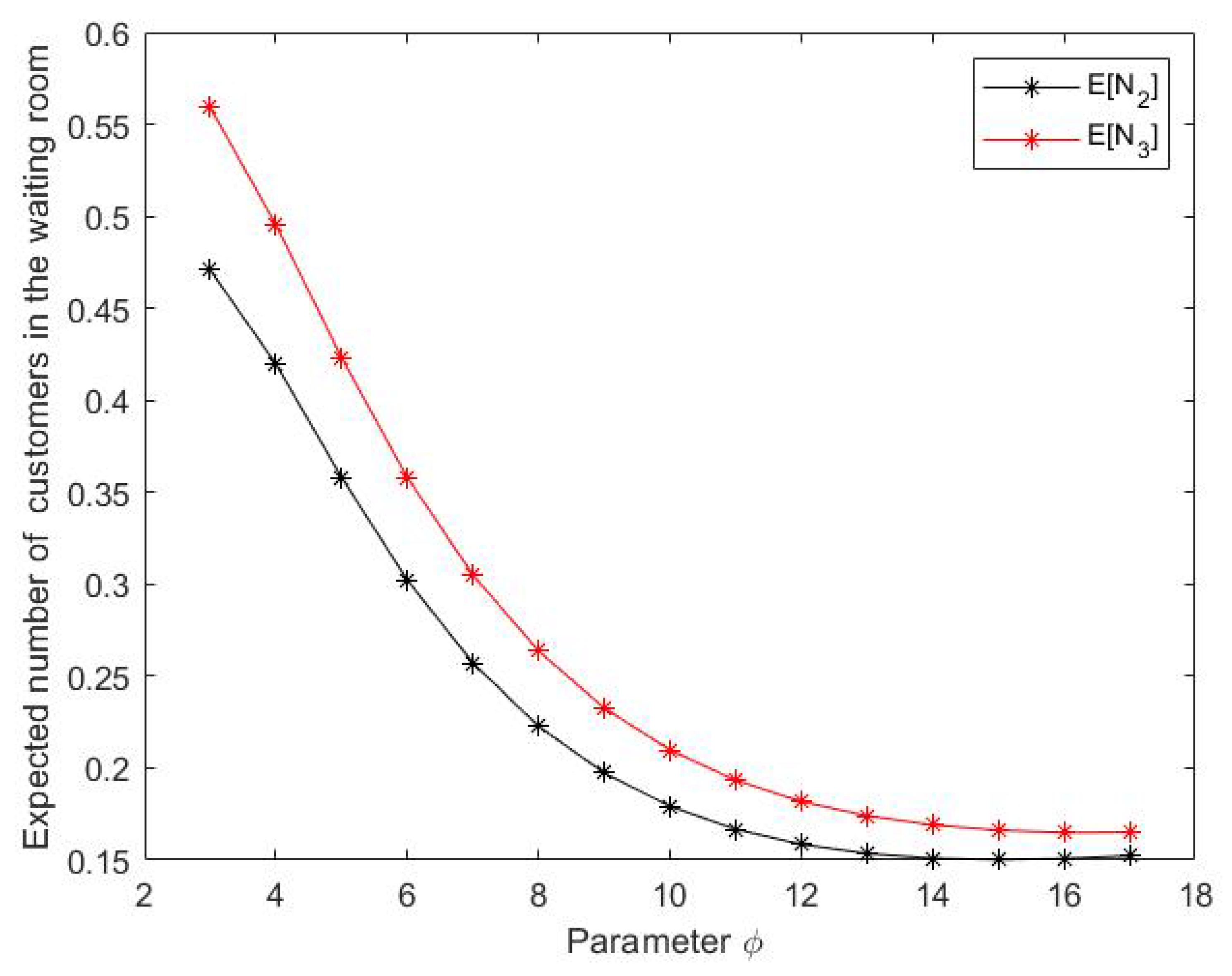
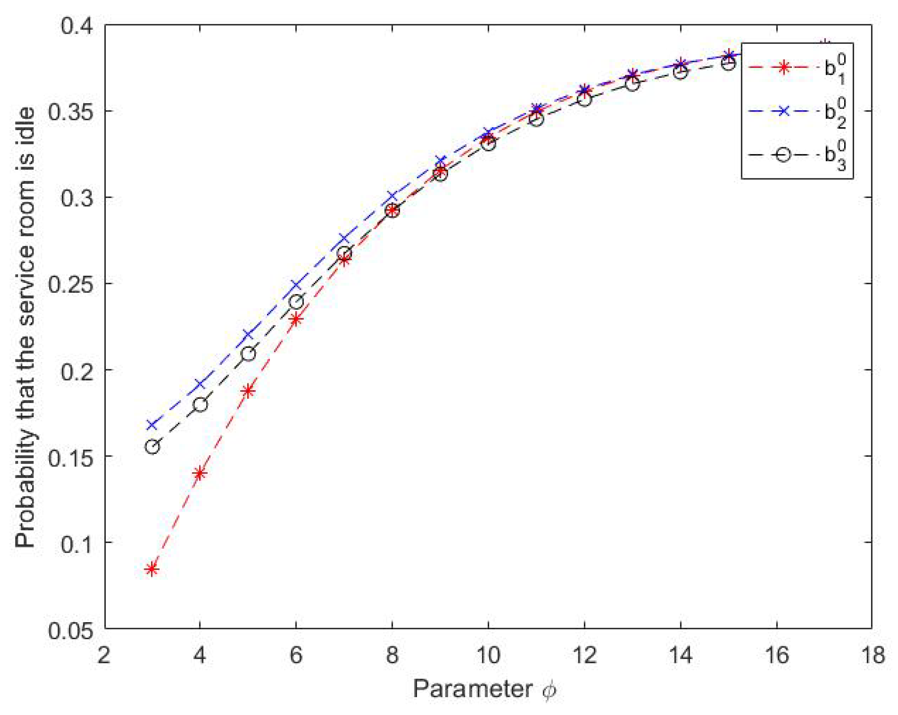
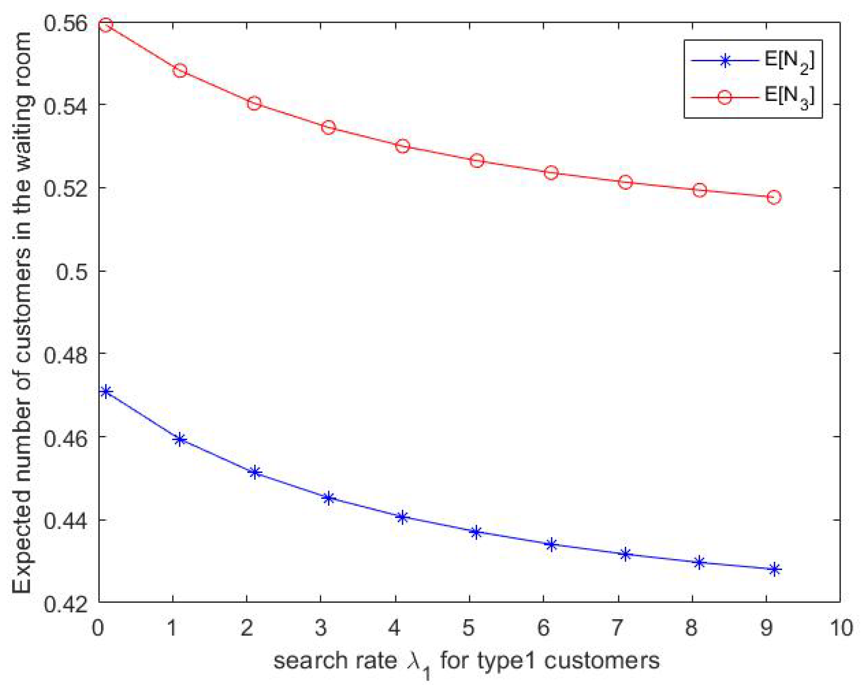
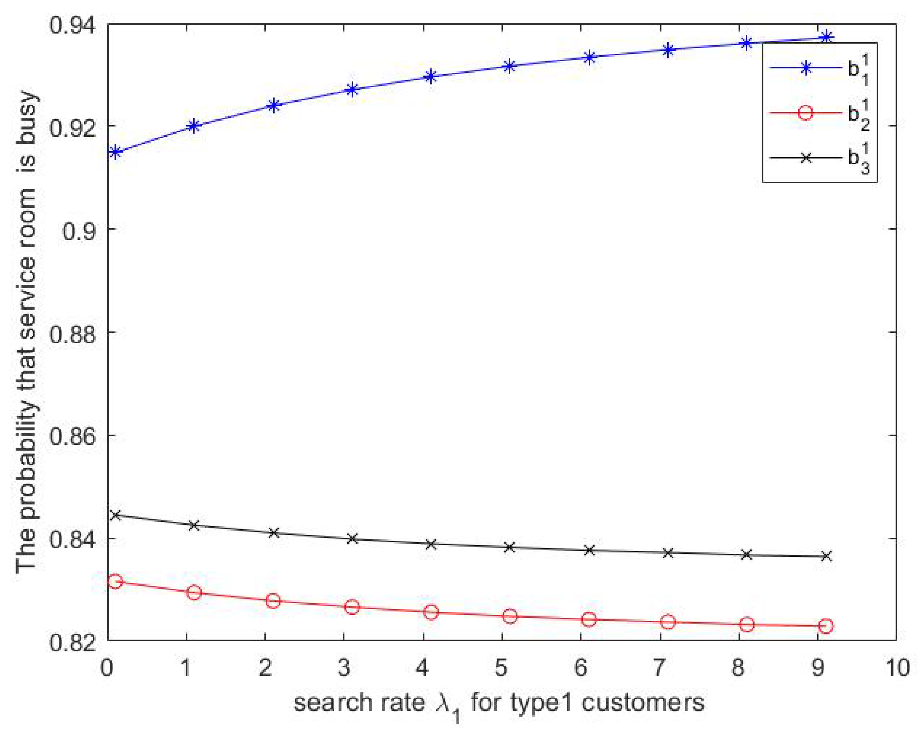
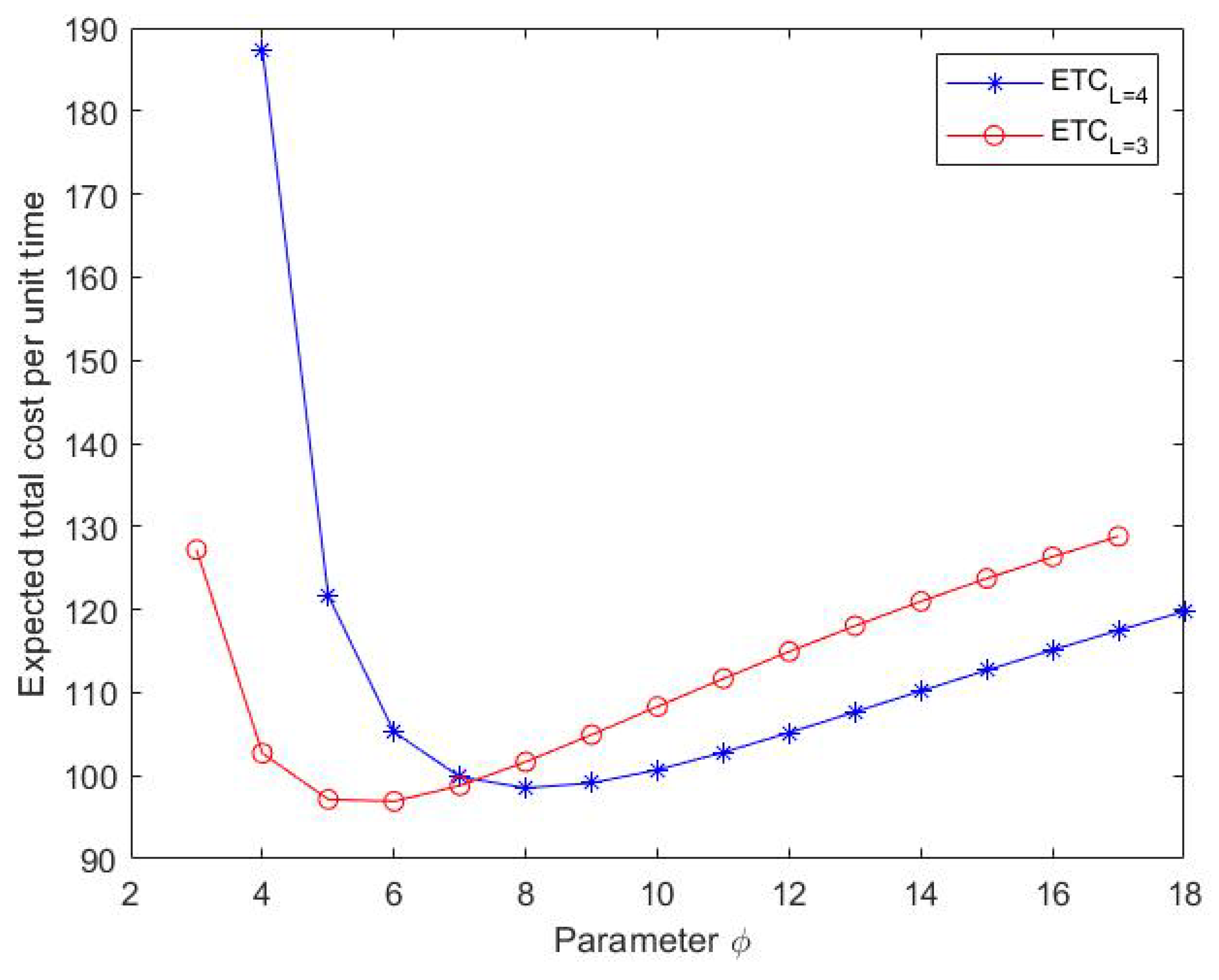
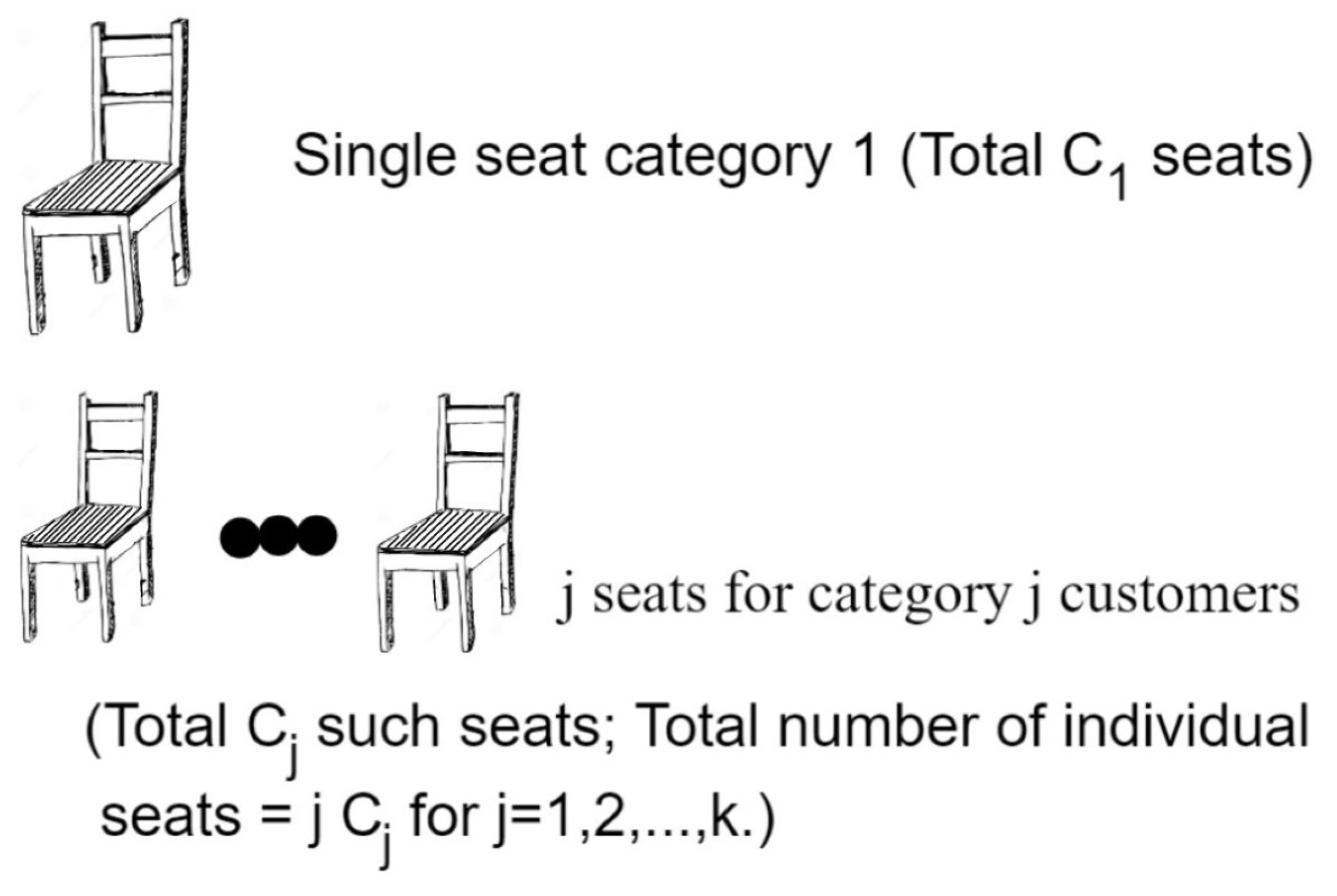
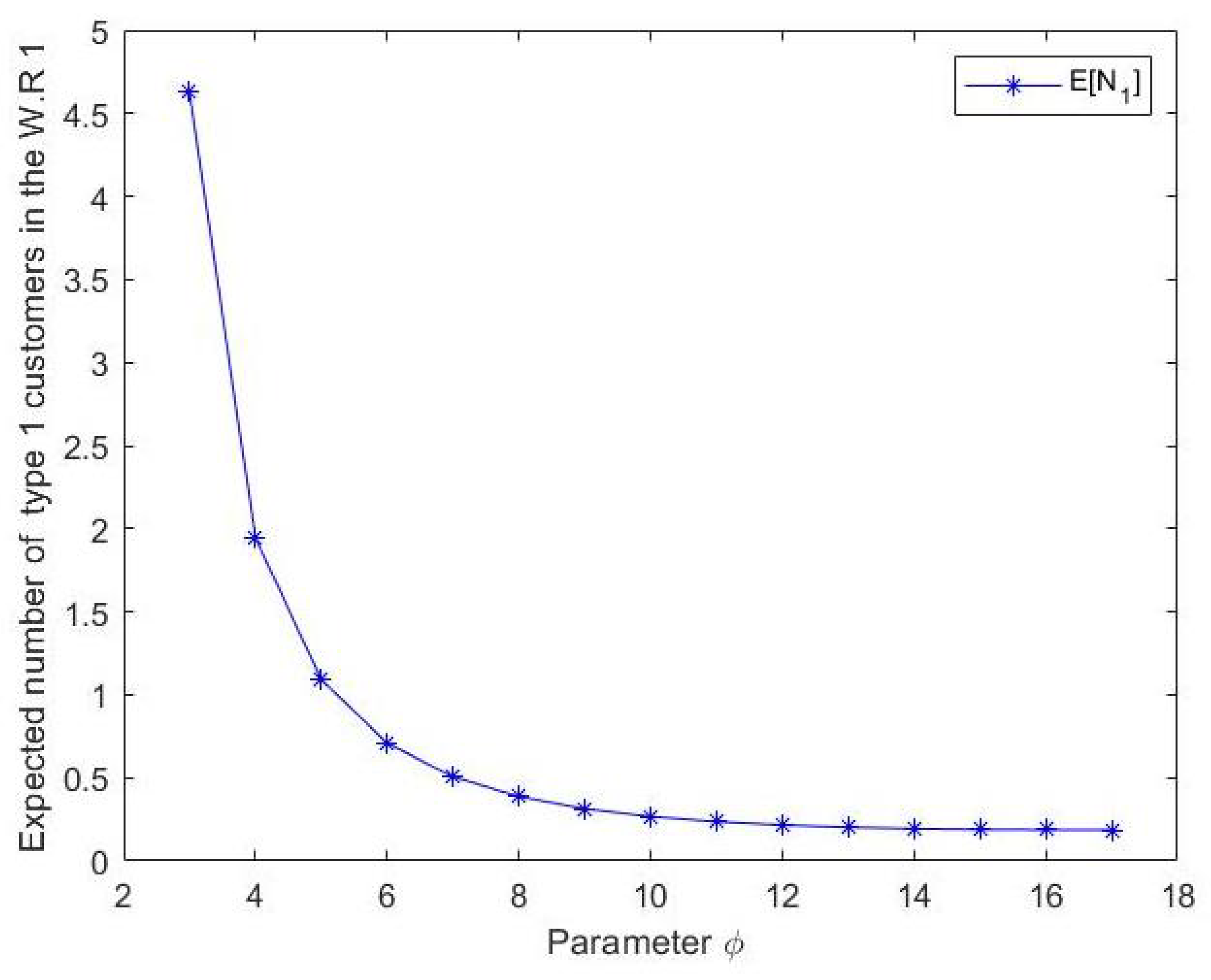
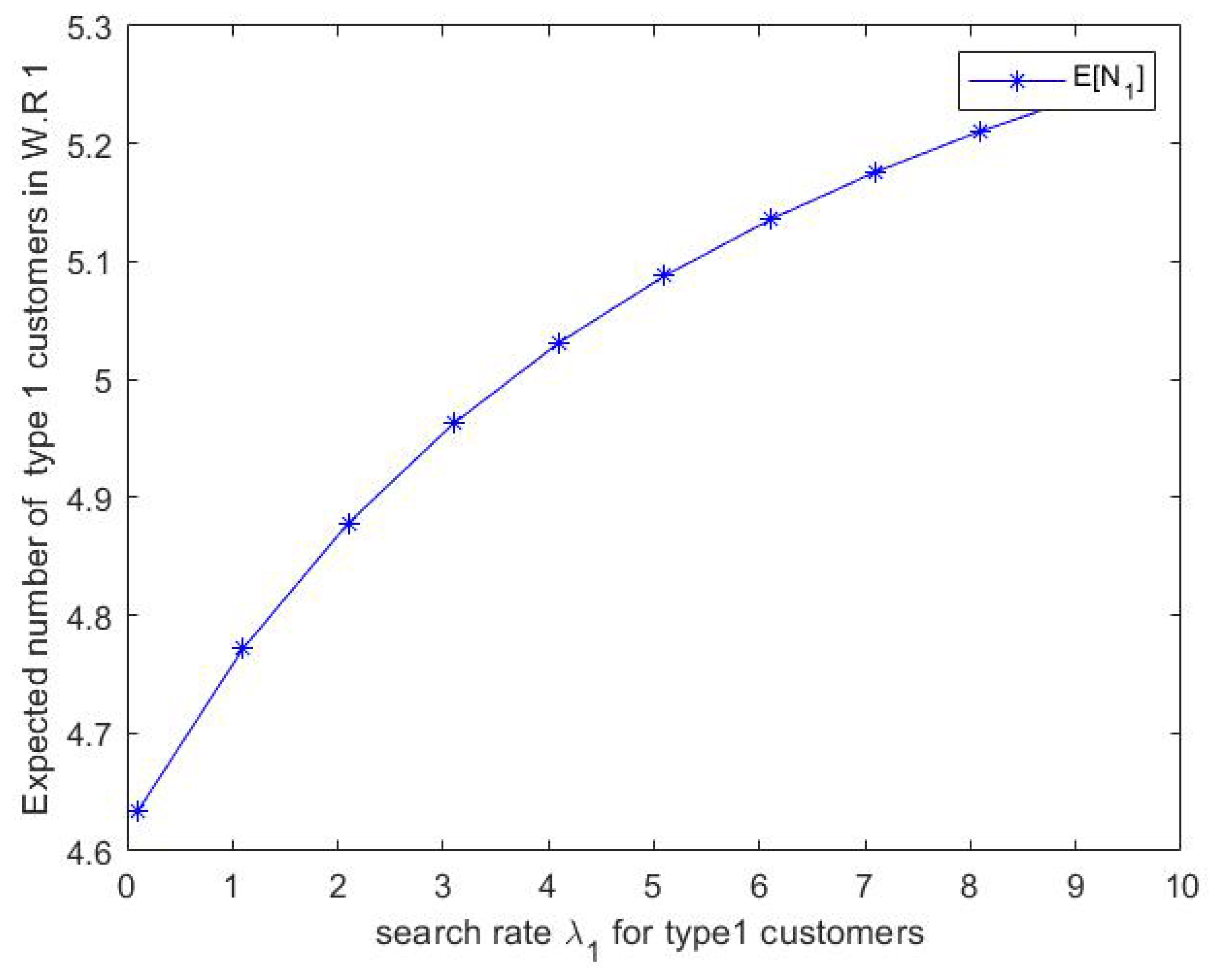
 ,
, 


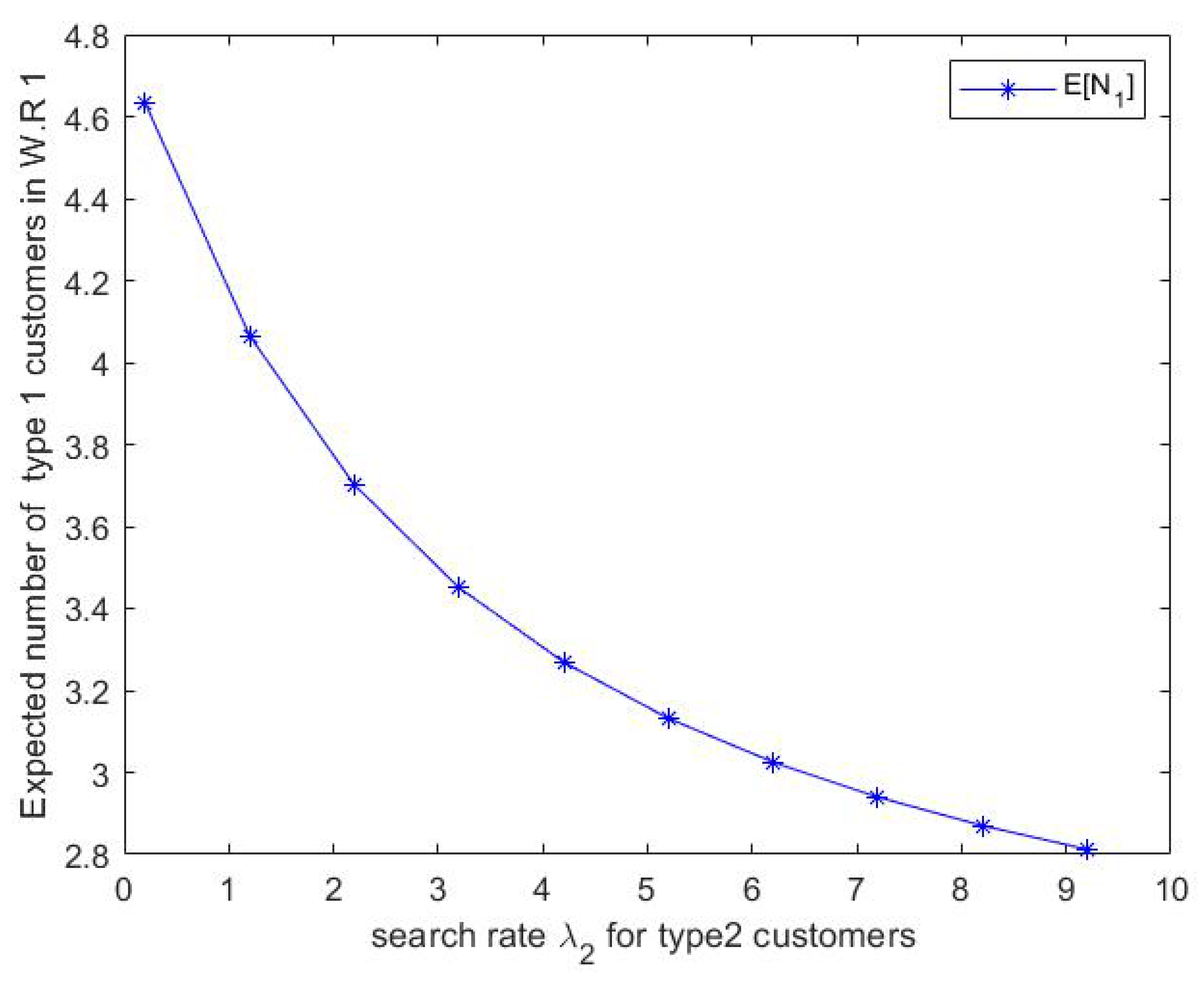
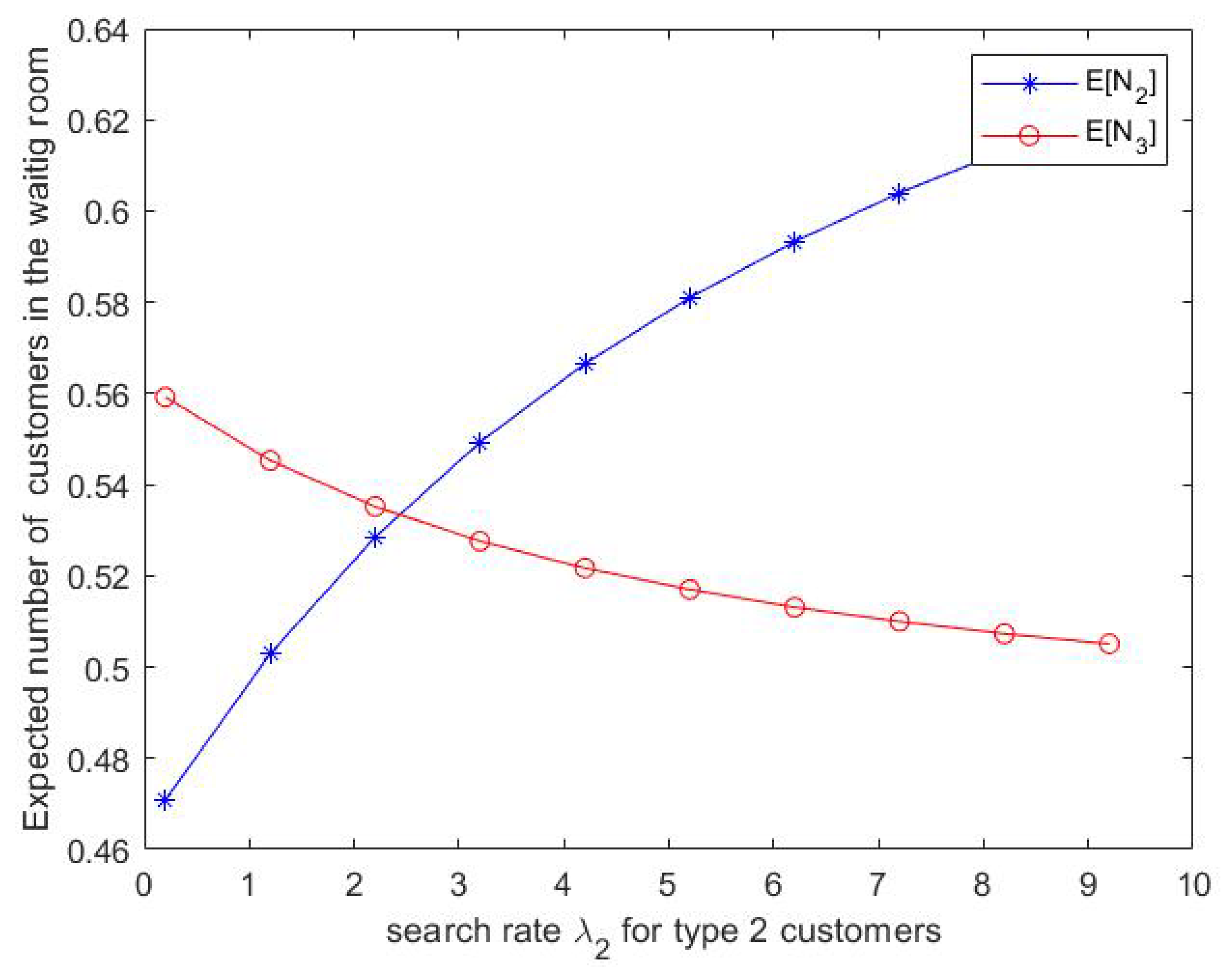
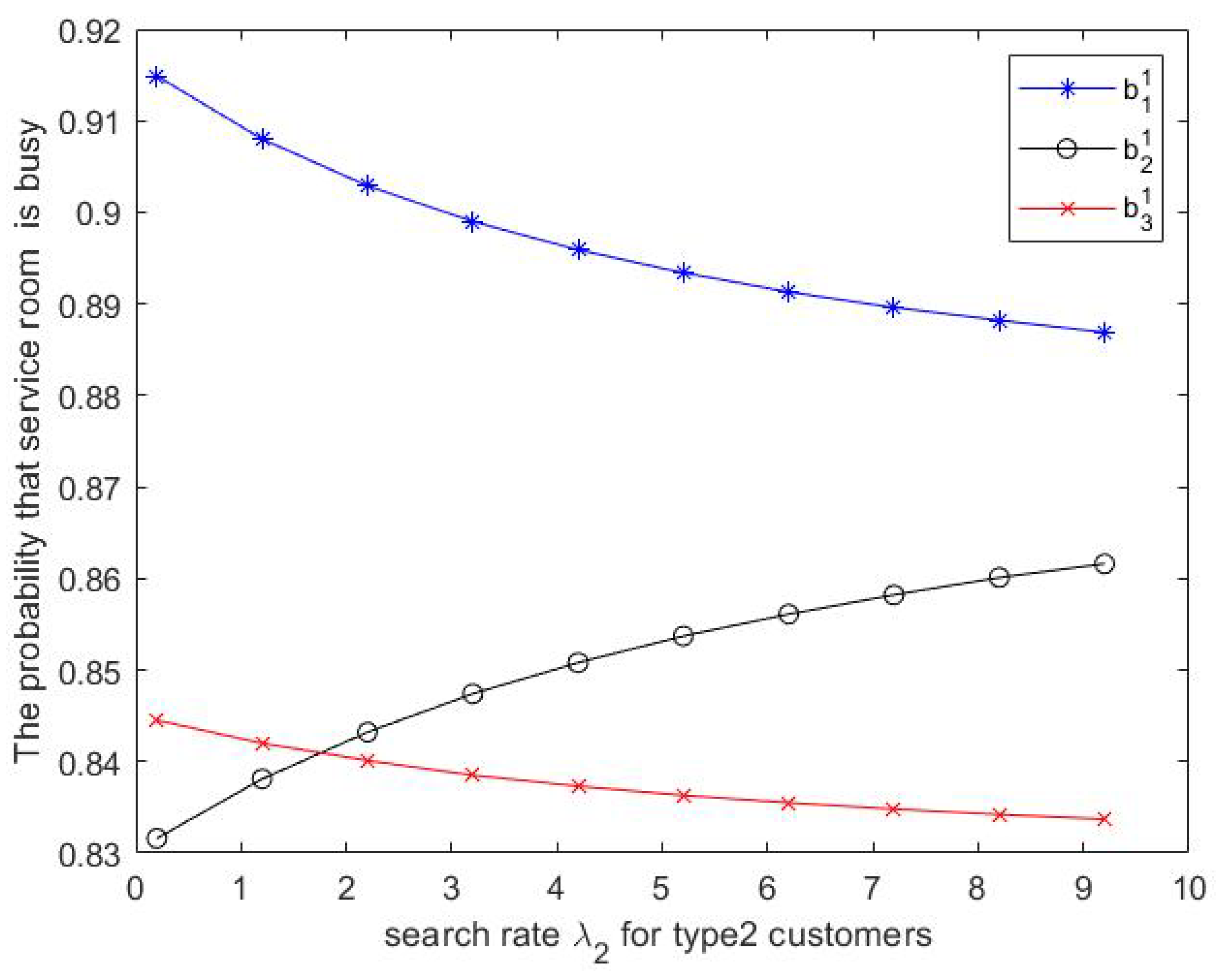
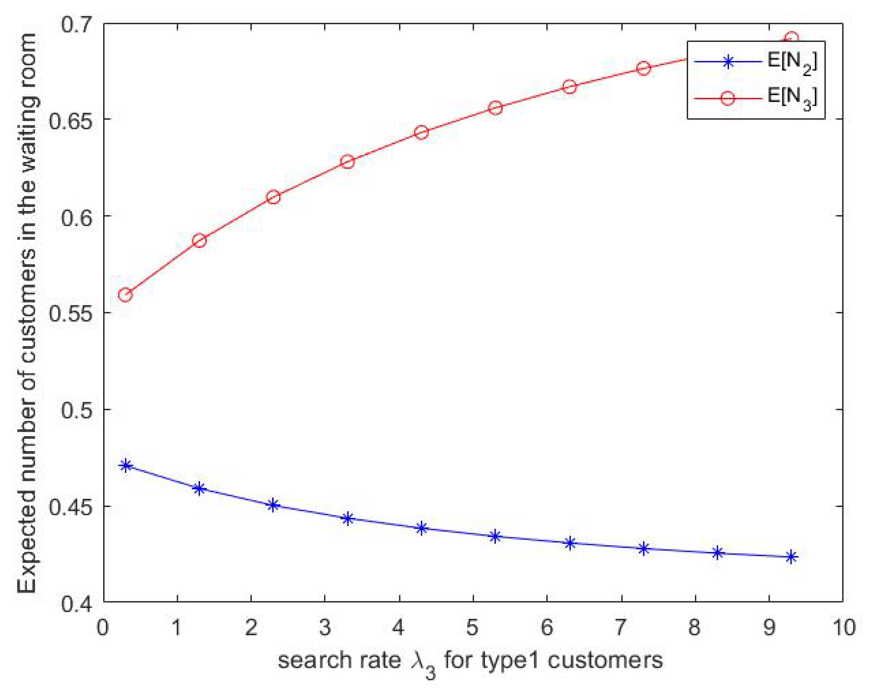
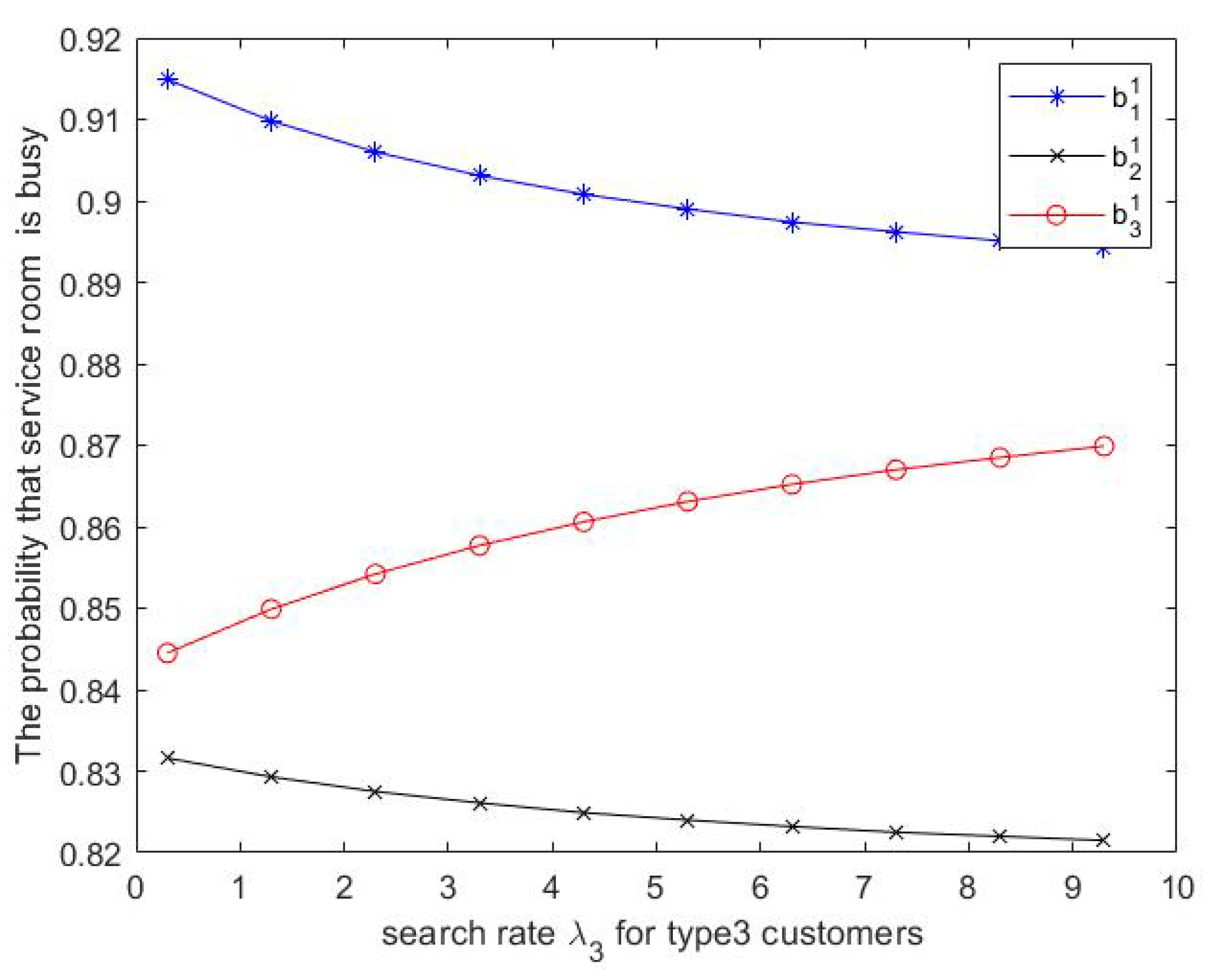