A Correct Benchmark Problem of a Two-Dimensional Droplet Deformation in Simple Shear Flow

Abstract

In this article, we numerically investigate a two-dimensional (2D) droplet deformation and breakup in simple shear flow using a phase-field model for two-phase fluid flows. The dominant driving force for a droplet breakup in simple shear flow is the three-dimensional (3D) phenomenon via surface tension force and Rayleigh instability, where a liquid cylinder of certain wavelengths is unstable against surface perturbation and breaks up into individual droplets to reduce the total surface energy. A 2D droplet breakup does not occur except in special cases because there is only one curvature direction of the droplet interface, which resists breakup. However, there have been many numerical simulation research works on the 2D droplet breakups in simple shear flow. This study demonstrates that the 2D droplet breakup phenomenon in simple shear flow is due to the lack of space resolution of the numerical grid.

1. Introduction

In this paper, we numerically investigate a two-dimensional (2D) droplet deformation and breakup in simple shear flow using a phase-field model for two-phase fluid flows. The dominant driving force for a droplet breakup is the three-dimensional (3D) phenomenon via surface tension force based on the mean curvature, which is the sum of the two principal curvatures, and Rayleigh instability, where a liquid cylinder of certain wavelengths is unstable against surface perturbation and breaks up into individual droplets to reduce the total surface energy [1,2,3]. See Figure 1 for an example of the temporal evolution of a 3D droplet shape under a simple shear flow.

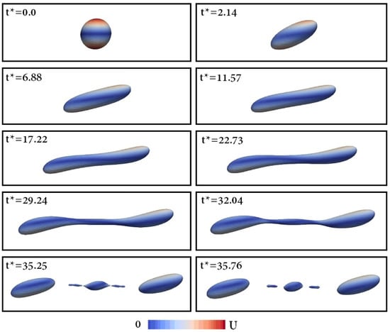
Figure 1. Temporal evolution of a 3D droplet shape under a simple shear flow. Reprinted from [4] with permission from Elsevier.

Komrakova et al. [5,6] numerically investigated the dynamics of a single liquid droplet suspended in another liquid in simple shear flow using the 3D lattice Boltzmann method (LBM). Wang et al. [7] studied the breakup of a droplet in simple shear flow with power-law rheology using a multiple-relaxation-time color-gradient LBM. Using a conservative, finite-volume, level-set method, Amani et al. [4] investigated the effect of the viscosity ratio on the dynamics of the breakup of a 3D droplet in simple shear flow. Liu et al. [8] investigated the breakup behavior of a 3D compound droplet in oscillatory shear flow using a 3D LBM. Recently, Wang and Ye [9] theoretically considered the energy conservation problem for the weak solutions to the 3D incompressible Navier–Stokes–Cahn–Hilliard system.

A 2D droplet breakup generally does not occur except special cases because there is only one curvature direction of the droplet interface, which resists breakup. However, there have been many numerical simulation research works on 2D droplet breakups. For example, Farokhirad et al. [10] studied droplet breakup in confined shear flow with various viscosity ratios, Reynolds numbers, and capillary numbers using the LBM based on the phase-field model. We can find more research papers [11,12,13], including a level set method about 2D droplet breakup under simple shear flow.

The novelty of this study is that it provides a guideline for validating newly developed two-dimensional numerical methods for simulating two-phase fluid flows with surface tension. A deformation test is a standard numerical benchmark problem for two-phase fluid flows. However, the non-physical 2D droplet breakup phenomenon is due to the lack of space resolution of the numerical grid. Therefore, it is essential to demonstrate the convergence of the 2D numerical solutions using the proposed schemes with sufficient grid points for the droplet deformation under a simple shear flow.

The paper is organized as follows. In Section 2, the governing equations and numerical solution algorithm is briefly described. In Section 3, several computational experiments are presented. In Section 4, conclusions are given.

2. Governing Equations and Numerical Solution

The governing equations are the Navier–Stokes–Cahn–Hilliard system [14,15,16,17,18,19,20,21,22]:

$$\begin{array}{ccc}\hfill \frac{\partial \mathbf{u}(\mathbf{x},t)}{\partial t}+\mathbf{u}(\mathbf{x},t)·\nabla \mathbf{u}(\mathbf{x},t)& =& -\nabla p(\mathbf{x},t)+\frac{1}{Re}\Delta \mathbf{u}(\mathbf{x},t)+\frac{1}{We}\mathbf{SF}(\mathbf{x},t),\hfill \end{array}$$

(1)

$$\begin{array}{ccc}\hfill \nabla ·\mathbf{u}(\mathbf{x},t)& =& 0,\hfill \end{array}$$

(2)

$$\begin{array}{ccc}\hfill \frac{\partial \varphi (\mathbf{x},t)}{\partial t}+\nabla ·\left(\varphi \right(\mathbf{x},t\left)\mathbf{u}\right(\mathbf{x},t\left)\right)& =& \frac{1}{Pe}\Delta [F^{\prime }\left(\varphi (\mathbf{x},t)\right)-{ϵ}^2\Delta \varphi (\mathbf{x},t)],\hfill \end{array}$$

(3)

where $\mathbf{u}(\mathbf{x},t)=\left(u\right(\mathbf{x},t),v(\mathbf{x},t\left)\right)$ is the velocity, $p(\mathbf{x},t)$ is the pressure, and $\varphi (\mathbf{x},t)$ is an order parameter at space $\mathbf{x}=(x,y)$ and time t. In addition, $F\left(\varphi \right)=0.25{({\varphi }^2-1)}^2$ is a double-well potential and $F^{\prime }\left(\varphi \right)$ is its derivative with respect to $\varphi$. In the two-phase fluids, the order parameter value $\varphi$ is close to one in one fluid and minus one in the other fluid. The dimensionless numbers $Re$, $We$, and $Pe$ are the Reynolds, Weber, and Peclet numbers, respectively. In addition, $\mathbf{SF}(\mathbf{x},t)$ is the surface tension force and is given by

$$\begin{array}{c}\hfill \mathbf{SF}(\mathbf{x},t)=(S{F}^x(\mathbf{x},t),S{F}^y(\mathbf{x},t))=-\frac{3\sqrt{2}}{4}\sigma ϵ\nabla ·\left(\frac{\nabla \varphi }{|\nabla \varphi |}\right)|\nabla \varphi |\nabla \varphi ,\end{array}$$

(4)

where $\sigma$ is a surface tension coefficient and $ϵ$ is an interfacial parameter that is related to the thickness of the interface transition layer and is the same as the parameter in Equation (3). In the phase-field model, to numerically resolve the interfacial transition efficiently and accurately, we use the $ϵ$ value, which is comparable to the numerical space step size. We can find a closed-form equation for the relation between the $ϵ$ value and the width of the transition layer in [23]. We note that there are many different formulas for the surface tension force. In this study, we choose Equation (4) for $\mathbf{SF}(\mathbf{x},t)$, which was derived using a geometrical approach of an interface profile such as curvature and a continuum method for modeling surface tension. In the continuum method [24], the surface tension force is written as $\mathbf{SF}(\mathbf{x},t)=\sigma \kappa \widehat{\mathbf{n}}\delta$, where the curvature of the interface $\kappa$, the normal vector $\widehat{\mathbf{n}}$, and the smoothed Dirac delta function $\delta$ correspond to $-\nabla ·\left(\nabla \varphi /|\nabla \varphi |\right)$, $\nabla \varphi /|\nabla \varphi |$, and ${0.75ϵ|\nabla \varphi |}^2$, respectively. More details about the derivation of the surface tension formula and comparison with the thermodynamically derived surface tension formula can be found in [25].

For completeness of exposition, we present the main numerical solution algorithm for the governing Equations (1)–(3). More details about the discretization can be found in [26]. Let us rewrite Equations (1) and (2) component-wise as

$$\begin{array}{ccc}\hfill \frac{\partial u(\mathbf{x},t)}{\partial t}& =& -u(\mathbf{x},t)u_x(\mathbf{x},t)-v(\mathbf{x},t)u_y(\mathbf{x},t)-p_x(\mathbf{x},t)+\frac{1}{Re}(u_{xx}(\mathbf{x},t)+u_{yy}(\mathbf{x},t))+\frac{1}{We}S{F}^x(\mathbf{x},t),\hfill \end{array}$$

(5)

$$\begin{array}{ccc}\hfill \frac{\partial v(\mathbf{x},t)}{\partial t}& =& -u(\mathbf{x},t)v_x(\mathbf{x},t)-v(\mathbf{x},t)v_y(\mathbf{x},t)-p_y(\mathbf{x},t)+\frac{1}{Re}(v_{xx}(\mathbf{x},t)+v_{yy}(\mathbf{x},t))+\frac{1}{We}S{F}^y(\mathbf{x},t),\hfill \end{array}$$

(6)

$$\begin{array}{ccc}\hfill u_x(\mathbf{x},t)& +& v_y(\mathbf{x},t)=0.\hfill \end{array}$$

(7)

Let $\mathsf{\Omega }=(L_x,R_x)\times (L_y,R_y)$ be a computational domain and be discretized as ${\mathsf{\Omega }}_h=\left\{(x_i,y_j)\right|x_i=L_x+(i-0.5)h,i=1,\cdots ,N_x \mathrm{and} y_j=L_y+(j-0.5)h,j=1,\cdots ,N_y\}$. Here, $N_x$ and $N_y$ are the positive integers and $h=(R_x-L_x)/N_x$ is the space grid size. In addition, we define ${\mathsf{\Omega }}_h^x=\left\{(x_i,y_j)\right|x_i=L_x+ih,i=0,\cdots ,N_x \mathrm{and} y_j=L_y+(j-0.5)h,j=1,\cdots ,N_y\}$ and ${\mathsf{\Omega }}_h^y=\left\{(x_i,y_j)\right|x_i=L_x+(i-0.5)h,i=1,\cdots ,N_x \mathrm{and} y_j=L_y+jh,j=0,\cdots ,N_y\}$ for the discrete u- and v-component momentum equations, respectively. On the discrete domains ${\mathsf{\Omega }}_h^x$ and ${\mathsf{\Omega }}_h^y$, Equations (5) and (6) are discretized as

$$\begin{array}{ccc}\hfill \frac{u_{i+\frac{1}{2},j}^{n+1}-u_{i+\frac{1}{2},j}^n}{\Delta t}& =& -{(u{u}_x+v{u}_y)}_{i+\frac{1}{2},j}^n-\frac{p_{i+1,j}^{n+1}-p_{ij}^{n+1}}{h}+\frac{1}{We}S{F}_{i+\frac{1}{2},j}^x\hfill \\ & & +\frac{1}{Re}\frac{u_{i-\frac{1}{2},j}^n+u_{i+\frac{3}{2},j}^n-4u_{i+\frac{1}{2},j}^n+u_{i+\frac{1}{2},j-1}^n+u_{i+\frac{1}{2},j+1}^n}{h^2},\hfill \end{array}$$

(8)

$$\begin{array}{ccc}\hfill \frac{v_{i,j+\frac{1}{2}}^{n+1}-v_{i,j+\frac{1}{2}}^n}{\Delta t}& =& -{(u{v}_x+v{v}_y)}_{i,j+\frac{1}{2}}^n-\frac{p_{i+1,j}^{n+1}-p_{ij}^{n+1}}{h}+\frac{1}{We}S{F}_{i,j+\frac{1}{2}}^y\hfill \\ & & +\frac{1}{Re}\frac{v_{i-1,j+\frac{1}{2}}^n+v_{i+1,j+\frac{1}{2}}^n-4v_{i,j+\frac{1}{2}}^n+v_{i,j-\frac{1}{2}}^n+v_{i,j+\frac{3}{2}}^n}{h^2}.\hfill \end{array}$$

(9)

To solve Equations (8) and (9), we apply a projection method [27]. First, we solve intermediate velocity fields ${\tilde{u}}_{i+\frac{1}{2},j}^{*}$ and ${\tilde{v}}_{i,j+\frac{1}{2}}^{*}$ without the following pressure term:

$$\begin{array}{ccc}\hfill \frac{{\tilde{u}}_{i+\frac{1}{2},j}^{*}-u_{i+\frac{1}{2},j}^n}{\Delta t}& =& -{(u{u}_x+v{u}_y)}_{i+\frac{1}{2},j}^n+\frac{1}{We}S{F}_{i+\frac{1}{2},j}^x\hfill \\ & & +\frac{1}{Re}\frac{u_{i-\frac{1}{2},j}^n+u_{i+\frac{3}{2},j}^n-4u_{i+\frac{1}{2},j}^n+u_{i+\frac{1}{2},j-1}^n+u_{i+\frac{1}{2},j+1}^n}{h^2},\hfill \end{array}$$

(10)

$$\begin{array}{ccc}\hfill \frac{{\tilde{v}}_{i,j+\frac{1}{2}}^{*}-v_{i,j+\frac{1}{2}}^n}{\Delta t}& =& -{(u{v}_x+v{v}_y)}_{i,j+\frac{1}{2}}^n+\frac{1}{We}S{F}_{i,j+\frac{1}{2}}^y\hfill \\ & & +\frac{1}{Re}\frac{v_{i-1,j+\frac{1}{2}}^n+v_{i+1,j+\frac{1}{2}}^n-4v_{i,j+\frac{1}{2}}^n+v_{i,j-\frac{1}{2}}^n+v_{i,j+\frac{3}{2}}^n}{h^2}.\hfill \end{array}$$

(11)

Next, we solve the following Poisson’s equation for the pressure field using a multigrid method [28]

$$\begin{array}{c}\hfill {\Delta }_d{p}_{ij}^{n+1}=\frac{1}{\Delta t}\left(\frac{{\tilde{u}}_{i+\frac{3}{2},j}^{*}-{\tilde{u}}_{i+\frac{1}{2},j}^{*}}{h}+\frac{{\tilde{v}}_{i,j+\frac{1}{2}}^{*}-{\tilde{v}}_{i,j-\frac{1}{2}}^{*}}{h}\right),\end{array}$$

(12)

where

$$\begin{array}{c}\hfill {\Delta }_d{p}_{ij}^{n+1}=\frac{p_{i-1,j}^{n+1}+p_{i+1,j}^{n+1}-4p_{ij}^{n+1}+p_{i,j-1}^{n+1}+p_{i,j+1}^{n+1}}{h^2}.\end{array}$$

(13)

Finally, we obtain the updated velocity fields:

$$\begin{array}{c}\hfill u_{i+\frac{1}{2},j}^{n+1}={\tilde{u}}_{i+\frac{1}{2},j}^{*}-\frac{\Delta t}{h}(p_{i+1,j}^{n+1}-p_{ij}^{n+1}),v_{i,j+\frac{1}{2}}^{n+1}={\tilde{v}}_{i,j+\frac{1}{2}}^{*}-\frac{\Delta t}{h}(p_{i,j+1}^{n+1}-p_{ij}^{n+1}).\end{array}$$

(14)

For the numerical solution of Equation (3), we use a finite difference method with the nonlinear multigrid method (see [29] more details about discretization, implementation, and its source C language code). In addition, the Fourier-spectral method for the CH equation can be found in [30] with a MATLAB source code.

3. Numerical Experiments

Now, we present several computational experiments to demonstrate that the 2D droplet breakup phenomenon is due to the lack of spatial resolution of the numerical grid. Let us define the interfacial-thickness-related parameter ${ϵ}_m=mh/\left[2\sqrt{2}{tanh}^{-1}\left(0.9\right)\right]$, which implies we have approximately $mh$ thickness across the interfacial transition layer if we use $ϵ={ϵ}_m$ [23].

We consider a droplet deformation in simple shear flow on a domain $\mathsf{\Omega }=(L_x,R_x)\times (L_y,R_y)$, as shown in Figure 2. Let us define the Taylor droplet deformation parameter $D=(L-B)/(L+B)$, where L and B are the maximum and minimum distances from the center of the droplet to the boundary of the droplet, respectively [31], see Figure 2. We use the periodic condition for the x-direction and no-slip boundary condition at the top and bottom of the domain with a wall velocity, i.e., $u(x,R_y,t)=R_y,v(x,R_y,t)=0$ and $u(x,L_y,t)=L_y,v(x,L_y,t)=0$. First, we compare the temporal evolution of the droplet deformation parameter with the results of [32]. For the initial state, the droplet radius is $R=0.5$, centered at $(0,0)$ in the computational domain $\mathsf{\Omega }=(-1,1)\times (-1,1)$. $N_x=N_y=64$, $\Delta t=0.0005$, $ϵ={ϵ}_5$, and $Pe=1/ϵ$ are used. The initial conditions are as follows:

$$\begin{array}{c}\hfill u(x,y,0)=y,v(x,y,0)=0,\varphi (x,y,0)=tanh\left(\frac{0.5-\sqrt{x^2+y^2}}{\sqrt{2}{ϵ}_5}\right).\end{array}$$

(15)

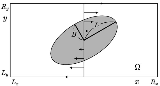
Figure 2. Schematic illustration of a droplet deformation in simple shear flow.

Figure 3 shows the evolution of the droplet deformation parameter D. The solid lines and symbols are results from [32], and the current phase-field method, respectively. Here, $Re=10$, $Ca=0.2,0.4,0.8$ are used. The capillary number is defined as $Ca=We/Re$. The numerical results from the two different computational methods are in good agreement with each other.

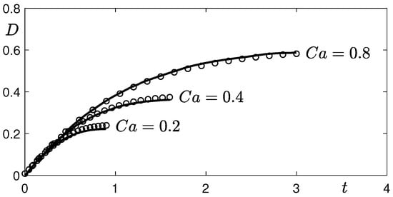
Figure 3. The evolution of the droplet deformation parameter $D=(L-B)/(L+B)$. The solid lines and symbols are the results from [32] and the current phase-field method, respectively. Here, $Re=10$, $Ca=0.2,0.4,0.8$ are used.

Next, we investigate the effect of the grid resolution on the temporal evolution of a droplet in simple shear flow. The initial conditions in the computational domain $\mathsf{\Omega }=(-3,3)\times (-1,1)$ are as follows:

$$\begin{array}{c}\hfill u(x,y,0)=y,v(x,y,0)=0,\varphi (x,y,0)=tanh\left(\frac{0.5-\sqrt{x^2+y^2}}{\sqrt{2}{ϵ}_5}\right).\end{array}$$

(16)

Here, $\Delta t=0.001$, $ϵ={ϵ}_5$, $Pe=1/ϵ$, $Re=100$, and $Ca=1$ are used. Figure 4a,b and Figure 5a,b show the temporal evolution of a droplet in simple shear flow with $96\times 32$, $192\times 64$, $384\times 128$, and $768\times 256$ grids, respectively. From top to bottom, times are at $t=0,0.7,5.25,5.95$, and 7. As shown in Figure 4a, if the grid is not sufficient, then the elongated droplet undergoes breakup, which is a non-physical phenomenon. However, as we further refine the grid by doubling the number of cells, then we can observe the elongated droplet without breakup. Note that we also reduce the value of the interfacial parameter as we refine the grid.

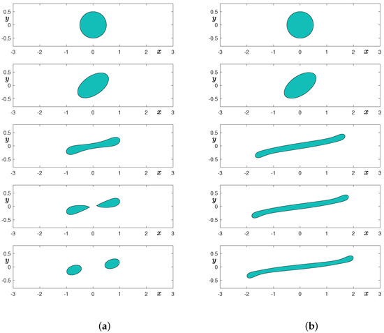
Figure 4. Temporal evolution of a droplet in shear flow: (a) $96\times 32$ grid and (b) $192\times 64$ grid. From top to bottom, times are at $t=0,0.7,5.25,5.95$, and 7.

Figure 6 shows a schematic illustration of the surface tension force of a deformed droplet in two-dimensional space. For better visualization, we normalize the magnitude of the surface tension force and only plot its direction. As shown in the figure, the direction of the surface tension force at the concave region is directed outward from the elongated droplet. Therefore, the two-dimensional elongated droplet cannot breakup at the concave region.

Figure 7 shows the convergence result at time $t=7$ for mesh refinement of the deformed droplet in simple shear flow with $96\times 32$, $192\times 64$, $384\times 128$, and $768\times 256$ grids. We can observe the interface of the elongated droplet converges as we further refine the mesh by doubling the number of cells.

Finally, we perform a computational experiment without fluid flow to clearly demonstrate the breakup phenomenon of an elongated droplet in 2D space. We only solve the following Cahn–Hilliard equation [33] on $\mathsf{\Omega }=(-3,3)\times (-1,1)$:

$$\begin{array}{c}\hfill \frac{\partial \varphi (\mathbf{x},t)}{\partial t}=\frac{1}{Pe}\Delta [F^{\prime }\left(\varphi (\mathbf{x},t)\right)-{ϵ}^2\Delta \varphi (\mathbf{x},t)],\end{array}$$

(17)

which is Equation (3) without the advection term. We use $Pe=1$, $\Delta t=0.01$, and $ϵ={ϵ}_5$. The initial condition is given as follows:

$$\begin{array}{c}\hfill \varphi (x,y,0)=\left\{\begin{array}{cc}1\hfill & \mathrm{if}\left|x\right|<2,\left|y\right|<0.125,\hfill \\ -1\hfill & \mathrm{otherwise}.\hfill \end{array}\right.\end{array}$$

(18)

Figure 5. Temporal evolution of a droplet in shear flow: (a) $384\times 128$ grid and (b) $768\times 256$ grid. From top to bottom, times are at $t=0,0.7,5.25,5.95$, and 7.

Figure 6. Schematic illustration of the surface tension force in two-dimensional space.

Figure 7. Convergence result at time $t=7$ for the mesh refinement of the deformed droplet in simple shear flow.

Figure 8a,b show the temporal evolution of a thin rectangular shape without fluid flow with $96\times 32$ and $192\times 64$ grids, respectively. It is well known that the dynamics of the Cahn–Hilliard equation do not preserve the convexity [34]. As shown in the second row of Figure 8, the shapes are not convex, even though they are initially convex. In the case of the coarse grid, we can observe that the initially thin rectangular shape undergoes a smoothing stage at the sharp corners and breakups into three smaller droplets. Furthermore, the largest droplet absorbs the smaller ones and results in a single drop. In the case of the finer grid, we can observe that the initially thin rectangular shape undergoes shape transformation into a droplet without topological change. Therefore, the breakup of an elongated shape in 2D is mainly due to insufficient grid resolution. We note that we may avoid this breakup phenomenon in 2D space if we use a conservative Alllen–Cahn equation that models the motion by mean curvature under mass conservation constraint [35].

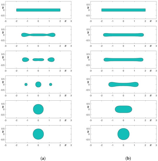
Figure 8. Temporal evolution of a thin rectangular shape without fluid flow: (a) $96\times 32$ grid and (b) $192\times 64$ grid. From top to bottom, times are at $t=0,0.3,0.4,2,6.4$, and 15.

4. Conclusions

In this article, we numerically investigated a 2D droplet deformation and breakup in simple shear flow using a phase-field model for two-phase fluid flows. The dominant driving force for a droplet breakup in simple shear flow is the 3D phenomenon via surface tension force and Rayleigh instability. A 2D droplet breakup does not occur except in special cases because there is only one curvature direction of the droplet interface, which directs outward from the elongated droplet at the concave region. Therefore, to validate a proposed numerical scheme of simulating 2D two-phase fluid flow with surface tension, mesh convergence tests should be performed until the elongated droplet does not breakup. In addition, it is essential to use an adaptive technique in two-phase fluid flow to resolve necessary resolution because of the multi-scale property [36]. As a future research topic, it would be interesting to investigate the 2D droplet breakup in the framework of the conservative Allen–Cahn equation [37,38]. Furthermore, the Taylor deformation rate D is only for the 3D case; to the authors’ knowledge, there is no theoretical Taylor deformation rate D of small deformation for the 2D case; therefore, it would be a good future research topic.

References

- Han, F. Cellular automata modeling of Ostwald ripening and Rayleigh instability. Materials 2018, 11, 1936. [Google Scholar] [CrossRef]
- Hao, X.; Zeng, Y. Simulation of Breakup Process of Polymer Jet during Melt Blowing. Fibers Polym. 2020, 21, 1222–1228. [Google Scholar] [CrossRef]
- Xie, L.; Yang, L.; Ye, H. Instability of gas-surrounded Rayleigh viscous jets: Weakly nonlinear analysis and numerical simulation. Phys. Fluids 2017, 29, 074101. [Google Scholar] [CrossRef]
- Amani, A.; Balcázar, N.; Castro, J.; Oliva, A. Numerical study of droplet deformation in shear flow using a conservative level-set method. Chem. Eng. Sci. 2019, 207, 153–171. [Google Scholar] [CrossRef]
- Komrakova, A.E.; Shardt, O.; Eskin, D.; Derksen, J.J. Lattice Boltzmann simulations of drop deformation and breakup in shear flow. Int. J. Multiph. Flow 2014, 59, 24–43. [Google Scholar] [CrossRef]
- Komrakova, A.E.; Shardt, O.; Eskin, D.; Derksen, J.J. Effects of dispersed phase viscosity on drop deformation and breakup in inertial shear flow. Chem. Eng. Sci. 2015, 126, 150–159. [Google Scholar] [CrossRef]
- Wang, N.; Liu, H.; Zhang, C. Deformation and breakup of a confined droplet in shear flows with power-law rheology. J. Rheol. 2017, 61, 741–758. [Google Scholar] [CrossRef]
- Liu, H.; Lu, Y.; Li, S.; Yu, Y.; Sahu, K.C. Deformation and breakup of a compound droplet in three-dimensional oscillatory shear flow. Int. J. Multiph. Flow 2021, 134, 103472. [Google Scholar] [CrossRef]
- Wang, Y.; Ye, Y. Energy conservation for weak solutions to the 3D Navier–Stokes–Cahn–Hilliard system. Appl. Math. Lett. 2022, 123, 107587. [Google Scholar] [CrossRef]
- Farokhirad, S.; Lee, T.; Morris, J.F. Effects of inertia and viscosity on single droplet deformation in confined shear flow. Commun. Comput. Phys. 2013, 13, 706–724. [Google Scholar] [CrossRef]
- Zhang, J.; Shu, S.; Guan, X.; Yang, N. Regime mapping of multiple breakup of droplets in shear flow by phase-field lattice Boltzmann simulation. Chem. Eng. Sci. 2021, 240, 116673. [Google Scholar] [CrossRef]
- Barai, N.; Mandal, N. Breakup modes of fluid drops in confined shear flows. Phys. Fluids 2016, 28, 073302. [Google Scholar] [CrossRef]
- Nazari, M.; Sani, H.M.; Kayhani, M.H.; Daghighi, Y. Different stages of liquid film growth in a microchannel: Two-phase Lattice Boltzmann study. Braz. J. Chem. Eng. 2018, 35, 977–994. [Google Scholar] [CrossRef]
- Adam, N.; Franke, F.; Aland, S. A Simple Parallel Solution Method for the Navier–Stokes Cahn–Hilliard Equations. Mathematics 2020, 8, 1224. [Google Scholar] [CrossRef]
- Bai, F.; Han, D.; He, X.M.; Yang, X. Deformation and coalescence of ferrodroplets in Rosensweig model using the phase field and modified level set approaches under uniform magnetic fields. Commun. Nonlinear Sci. Numer. Simul. 2020, 85, 105213. [Google Scholar] [CrossRef]
- Chen, Y.; Huang, Y.; Yi, N. Error analysis of a decoupled, linear and stable finite element method for Cahn–Hilliard–Navier–Stokes equations. Appl. Math. Comput. 2022, 421, 126928. [Google Scholar] [CrossRef]
- Chen, L.; Zhao, J. A novel second-order linear scheme for the Cahn–Hilliard–Navier–Stokes equations. J. Comput. Phys. 2020, 423, 109782. [Google Scholar] [CrossRef]
- Guo, Z.; Cheng, Q.; Lin, P.; Liu, C.; Lowengrub, J. Second order approximation for a quasi-incompressible Navier–Stokes Cahn–Hilliard system of two-phase flows with variable density. J. Comput. Phys. 2022, 448, 110727. [Google Scholar] [CrossRef]
- Dehghan, M.; Gharibi, Z. Numerical analysis of fully discrete energy stable weak Galerkin finite element Scheme for a coupled Cahn–Hilliard–Navier–Stokes phase-field model. Appl. Math. Comput. 2021, 410, 126487. [Google Scholar] [CrossRef]
- Li, M.; Xu, C. New efficient time-stepping schemes for the Navier–Stokes–Cahn–Hilliard equations. Comput. Fluids 2021, 231, 105174. [Google Scholar] [CrossRef]
- Liu, C.; Frank, F.; Thiele, C.; Alpak, F.O.; Berg, S.; Chapman, W.; Riviere, B. An efficient numerical algorithm for solving viscosity contrast Cahn–Hilliard–Navier–Stokes system in porous media. J. Comput. Phys. 2020, 400, 108948. [Google Scholar] [CrossRef]
- Sohaib, M.; Shah, A. Fully decoupled pressure projection scheme for the numerical solution of diffuse interface model of two-phase flow. Commun. Nonlinear Sci. Numer. Simul. 2022, 112, 106547. [Google Scholar] [CrossRef]
- Choi, J.W.; Lee, H.G.; Jeong, D.; Kim, J.S. An unconditionally gradient stable numerical method for solving the Allen–Cahn equation. Phys. A 2009, 388, 1791–1803. [Google Scholar] [CrossRef]
- Brackbill, J.U.; Kothe, D.B.; Zemach, C. A continuum method for modeling surface tension. J. Comput. Phys. 1992, 100, 335–354. [Google Scholar] [CrossRef]
- Kim, J.S. A continuous surface tension force formulation for diffuse-interface models. J. Comput. Phys. 2005, 204, 784–804. [Google Scholar] [CrossRef]
- Kim, J.S. Phase-Field Models for Multi-Component Fluid Flows. Comm. Comput. Phys. 2012, 12, 613–661. [Google Scholar] [CrossRef]
- Chorin, A.J. Numerical Solution of the Navier–Stokes Equations. Math. Comput. 1968, 22, 745–762. [Google Scholar] [CrossRef]
- Trottenberg, U.; Oosterlee, C.W.; Schüller, A. Multigrid; Academic Press: New York, NY, USA, 2001. [Google Scholar]
- Lee, C.; Jeong, D.; Yang, J.; Kim, J. Nonlinear multigrid implementation for the two-dimensional Cahn–Hilliard equation. Mathematics 2020, 8, 97. [Google Scholar] [CrossRef]
- Yoon, S.; Jeong, D.; Lee, C.; Kim, H.; Kim, S.; Lee, H.G.; Kim, J.S. Fourier-spectral method for the phase-field equations. Mathematics 2020, 8, 1385. [Google Scholar] [CrossRef]
- Chen, Y.; Liang, Y.; Chen, M. The deformation and breakup of a droplet under the combined influence of electric field and shear flow. Fluid Dyn. Res. 2021, 53, 065504. [Google Scholar] [CrossRef]
- Sheth, K.S.; Pozrikidis, C. Effects of inertia on the deformation of liquid drops in simple shear flow. Comput. Fluids 1995, 24, 101–119. [Google Scholar] [CrossRef]
- Li, Y.; Wang, J. Unconditional convergence analysis of stabilized FEM-SAV method for Cahn–Hilliard equation. Appl. Math. Comput. 2022, 419, 126880. [Google Scholar] [CrossRef]
- Lee, D.; Kim, J.S. Comparison study of the conservative Allen–Cahn and the Cahn–Hilliard equations. Math. Comput. Simul. 2016, 119, 35–56. [Google Scholar] [CrossRef]
- Cui, C.; Liu, J.; Mo, Y.; Zhai, S. An effective operator splitting scheme for two-dimensional conservative nonlocal Allen–Cahn equation. Appl. Math. Lett. 2022, 130, 108016. [Google Scholar] [CrossRef]
- Barosan, I.; Anderson, P.D.; Meijer, H.E.H. Application of mortar elements to diffuse-interface methods. Comput. Fluids 2006, 35, 1384–1399. [Google Scholar] [CrossRef]
- Liu, P.; Ouyang, Z.; Chen, C.; Yang, X. A novel fully-decoupled, linear, and unconditionally energy-stable scheme of the conserved Allen–Cahn phase-field model of a two-phase incompressible flow system with variable density and viscosity. Commun. Nonlinear Sci. Numer. Simul. 2022, 107, 106120. [Google Scholar] [CrossRef]
- Kwak, S.; Yang, J.; Kim, J.S. A conservative Allen–Cahn equation with a curvature-dependent Lagrange multiplier. Appl. Math. Lett. 2022, 126, 107838. [Google Scholar] [CrossRef]
Publisher’s Note: MDPI stays neutral with regard to jurisdictional claims in published maps and institutional affiliations. |
© 2022 by the authors. Licensee MDPI, Basel, Switzerland. This article is an open access article distributed under the terms and conditions of the Creative Commons Attribution (CC BY) license (https://creativecommons.org/licenses/by/4.0/).