On an Application of Lattice Integral Transforms in Image Processing ^†

Abstract

The lattice integral transforms have been introduced to generalize lower and upper fuzzy transforms for lattice-valued functions that are used to approximate original functions from below and above. They are defined in complete analogy with classical integral transforms, particularly, the product of a lattice-valued function and a fuzzy relation called the integral kernel is integrated by a Sugeno-like fuzzy integral. In the article, we first investigate the conditions under which lattice integral transforms preserve (reverse) constant functions, which appears to be a fundamental presumption for a successful approximation of lattice-valued functions. Further, we show how the lattice integral transforms can be applied in image processing, more specifically, in non-linear filtering, compression/decompression, and opening/closing of images. We demonstrate that the filters based on integral transforms generalize the popular median filter as well as minimum and maximum filters, and also opening and closing defined using fuzzy morphological erosion and dilation. We illustrate the proposed methods in various selected images.

1. Introduction

In [1], integral transforms for lattice-valued functions (lattice integral transforms or simply integral transforms) have been introduced to provide a theoretical framework for transformations of functions whose functional values cannot, in principle, be handled by standard arithmetic of real or complex numbers or application of standard arithmetic has certain disadvantages. For example, non-additive noise in signal or image processing is filtered out by methods that do not use the standard arithmetic, but order statistic functions, such as median, are applied (see, e.g., [2]). Mathematical morphology on complete lattices provides morphological operators whose mathematically coherent application to grayscale images has already been justified (see, e.g., [3,4,5]). The scheme of lattice integral transforms is designed quite analogously to classical integral transforms, such as Fourier, Laplace, Hilbert, or wavelet transforms [6]. Namely, a new function $g(y)$ is created by integrating the product of a function $f(x)$ and an integral kernel function $K(x,y)$ with respect to suitable limits. To develop the theory of lattice integral transforms in sufficient generality, the complete residuated lattices were chosen as the basic algebraic structure for the function values. Recall that particular examples of residuated lattices are the BL-algebra, MV-algebra, or IMTL-algebra, which are very popular in fuzzy set theory, fuzzy logic, and their applications.

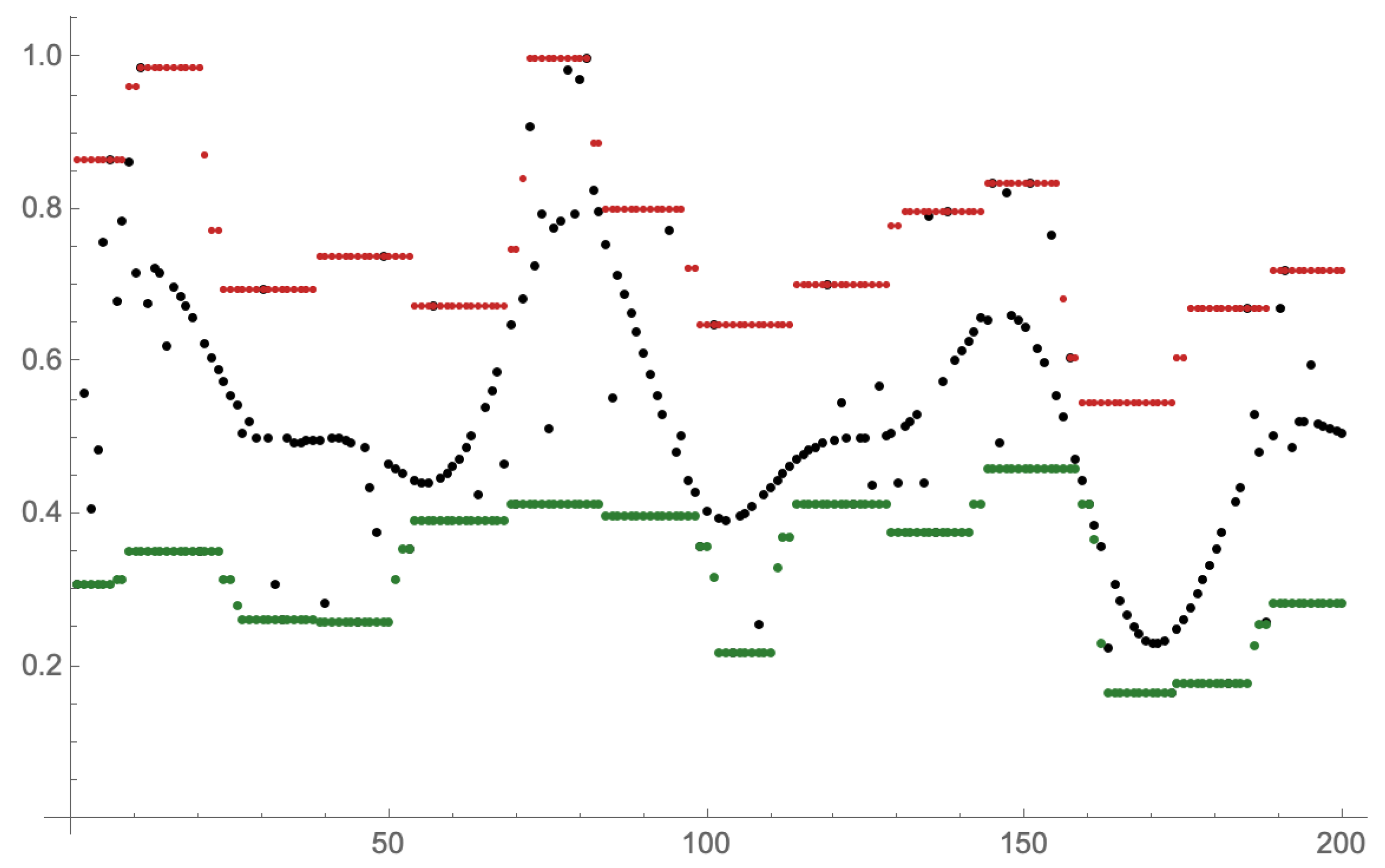
The original motivation for introducing lattice integral transforms arose from the idea of generalizing fuzzy transforms of lattice-valued functions (lattice fuzzy transforms) that Perfilieva proposed in [7] to approximate functions from below or above using the appropriate composition of the direct upper (lower) fuzzy transform $F^{\uparrow }(F^{\downarrow }):\mathcal{F}(X)\to \mathcal{F}(Y)$ and the inverse upper (lower) fuzzy transform $G^{\uparrow }(G^{\downarrow }):\mathcal{F}(Y)\to \mathcal{F}(X)$, where $\mathcal{F}(X)$ is the set of all lattice-valued functions on X and similarly for $\mathcal{F}(Y)$. The key parameter of lattice fuzzy transforms $F^{\uparrow }$ and $F^{\downarrow }$ is the fuzzy partition of the domain X of functions that are approximated, which is a family of fuzzy subsets of X whose cores are non-empty sets and form a classical partition of X. Note that the core of a fuzzy set A on X is the set of all elements of X for which the membership function of A gives 1. It should be noted that the fuzzy transforms of the lattice $G^{\uparrow }$ and $G^{\downarrow }$ are also determined by a fuzzy partition of Y, which is derived from the fuzzy partition of X. Hence, we find that there is no difference in the definitions of $F^{\uparrow }$ and $G^{\downarrow }$ ($F^{\downarrow }$ and $G^{\uparrow }$) and it is unnecessary to distinguish between the definitions of direct and inverse lattice fuzzy transforms. The approximation of original lattice-valued functions is controlled by setting of fuzzy partitions of the domain X. Note that fuzzy partitions of the domain Y do not form another approximation parameter, because they are derived from fuzzy partitions of the domain X. On Figure 1 (the figure is adopted from [8]), the lower and upper approximations of a discrete function are displayed for a uniform fuzzy partition of the domain $[0,200]$ which is determined by moving a fuzzy set along the x-axis with the size of its core equal to 15.

Further development of lattice fuzzy transforms, including details, can be found in [9,10,11,12,13,14]. The relationship between fuzzy lattice transforms and fuzzy morphological operators defined on complete lattices was demonstrated by Sussner in [15]. In particular, $F^{\uparrow }$ and $G^{\downarrow }$ ($F^{\downarrow }$ and $G^{\uparrow }$) have been shown to be equivalent to fuzzy morphological dilation (erosion).

The proposed integral transforms for lattice-valued functions naturally extend the lattice fuzzy transforms in two directions, namely, the fuzzy partition is replaced by a more general concept of integral kernel, and the supremum and infimum used in the calculation of fuzzy transforms are replaced by Sugeno-like fuzzy integrals. More specifically, two types of lattice integral transforms from $\mathcal{F}(X)$ to $\mathcal{F}(Y)$ were introduced using the following formula [1]:

$$\begin{array}{c}{F}_{(K,\mu )}^{\otimes }(f)(y)={\int }_{X}K(x,y)\otimes f(x)d\mu \mathrm{and}{F}_{(K,\mu )}^{\to }(f)(y)={\int }_{X}K(x,y)\to f(x)d\mu ,\end{array}$$

where $K:X\times Y\to L$ is a fuzzy relation called the integral kernel and ${\int }_X$ is a multiplication-based Sugeno-like fuzzy integral on a fuzzy measure space $(X,\mathcal{A},\mu )$. It was shown that $F_{(K,\mu )}^{\otimes }$ generalizes the upper lattice fuzzy transform $F^{\uparrow }$ and $F_{(K,\mu )}^{\to }$ the lower lattice fuzzy transform $F^{\downarrow }$. More specifically, we have the following:

$$\begin{array}{c}{F}^{\uparrow }=F_{(K,{\mu }^{\top })}^{\otimes }\mathrm{and}{F}^{\downarrow }=F_{(K,{\mu }^{\perp })}^{\to }\end{array}$$

where ${\mu }^{\perp }$ is the least fuzzy measure and ${\mu }^{\top }$ is the highest fuzzy measure on $\mathcal{A}$ which is given on the powerset of X (see Example 5 on p. 5 for the definition of ${\mu }^{\perp }$ and ${\mu }^{\top }$). The same formula, but with residuum-based Sugeno-like fuzzy integrals, were used in the definitions of other types of lattice integral transforms in [16]. Similarly to the lattice fuzzy transforms, in the current paper [17], we show that different compositions of the integral transforms

$$\begin{array}{c}{F}_{(K,\mu )}^{\otimes }:\mathcal{F}(X)\to \mathcal{F}(Y)\mathrm{and}{F}_{(K^{-1},{\mu }^{\prime })}^{\to }:\mathcal{F}(Y)\to \mathcal{F}(X),\end{array}$$

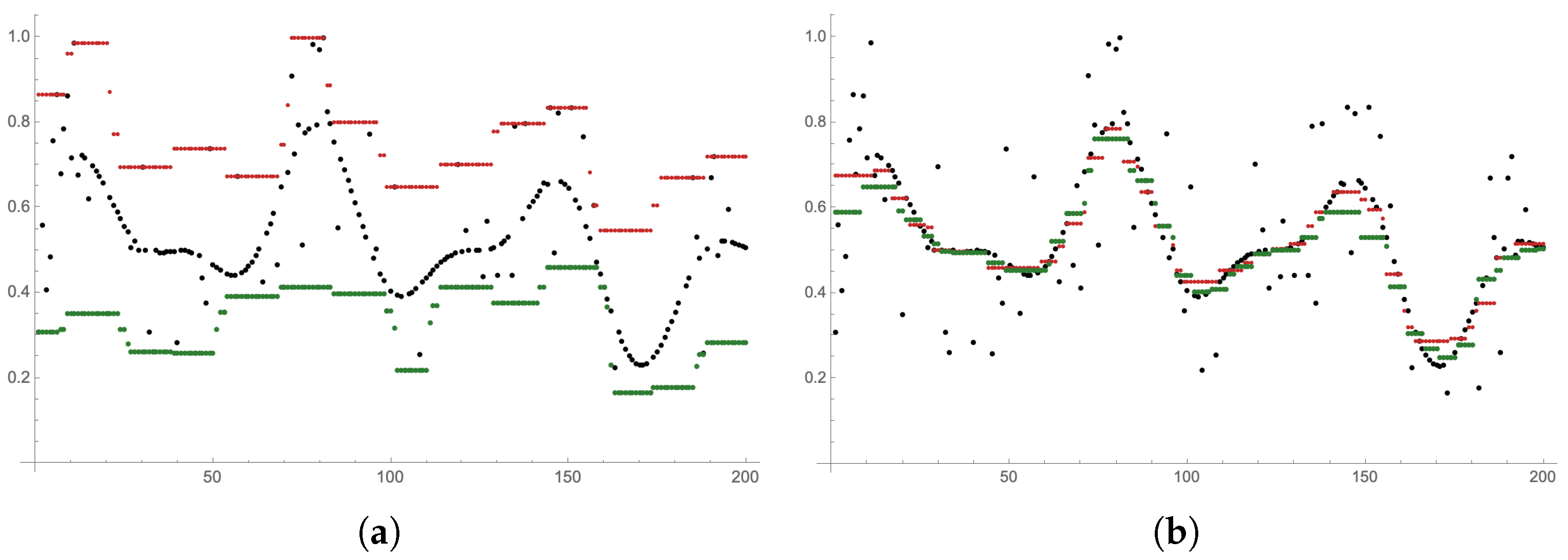
where $K^{-1}:Y\times X\to L$ is given by $K^{-1}(y,x)=K(x,y)$ and ${\mu }^{\prime }$ is an appropriate fuzzy measure on a fuzzy measurable space $(Y,\mathcal{G})$, approximate the original functions, and can also remove the present random noise, in contrast to the fuzzy transform, as shown in Figure 2. This valuable property motivated us to apply integral transformations in image processing, specifically to image filtering and compression/decompression in the current paper [8], where we outline the prerequisites to obtain successful results for these tasks and illustrate them with the Lena image. Another application of the integral transformation based on multiplication was proposed for multi-criteria decision-making in [18], where the integral transform is used to evaluate goals according to respondents’ fulfillment and significance of criteria, where the significance of criteria with respect to goals is expressed by an integral kernel. Both applications show the natural directions of using lattice integral transforms in practice, i.e., signal and image processing and multi-criteria decision-making, but a deeper analysis of the performance and usefulness of integral transforms in these and possibly other applications is still a subject of research.

This paper is a continuation of our research on signal reconstruction by lattice integral transforms starting in [17] and, especially, the image processing application provided in [8]. More specifically, we extend the ideas and complete results presented in [8] (and also in [17]) to obtain a comprehensive background for image (and also signal) processing. Particularly, we present two types of lattice integral transforms and prove their fundamental properties that ensure a successful application to image processing. In the illustration, we focus on three tasks in image processing, namely, non-linear filtering, compression/decompression, and opening/closing of images. Among other things, we show that non-linear filters based on lattice integral transforms can be seen as a generalization of the known median filter, as well as minimum and maximum filters. Note that these filters are popular for the removal of salt-and-pepper noise, more specifically, the minimum (maximum) filter removes the salt (pepper) noise because it has very high (low) values of intensities. The median filter removes both types of noise. The minimum and maximum filters are also associated with the most common morphological operations of erosion and dilation, because the minimum filter erodes shapes on the image, whereas the maximum filter extends object boundaries [19]. The opening and closing filters are achieved by combining the morphological operations of erosion and dilation, in our case, we will consider their definitions in fuzzy mathematical morphology [15].

The structure of the paper is as follows. The next section presents basic concepts that are used in the construction of lattice integral transforms. The third section introduces two types of lattice integral transforms, which are defined using the multiplication and residuum-based fuzzy integrals. The fourth section is devoted to three tasks in image processing, namely, non-linear noise filtering, compression/decompression and opening/closing, which are designed in the framework of lattice integral transforms and demonstrated on various images. The last section is a conclusion.

2. Preliminary

In this section, we present all concepts that are important to introduce lattice integral transforms. Some of them are demonstrated by examples.

2.1. Algebra of Truth Values

In this paper, we assume that the algebra of truth values is a complete residuated lattice on $[0,1]$, i.e., an algebra $L=\langle [0,1],\wedge ,\vee ,\otimes ,\to ,0,1\rangle$ with four binary operations and two constants, such that $\langle [0,1],\wedge ,\vee \rangle$ is a complete lattice, $\langle [0,1],\otimes ,1\rangle$ is a commutative monoid (i.e., ⊗ is associative, commutative and the identity $\alpha \otimes 1=\alpha$ holds for any $\alpha \in [0,1]$) and the adjointness property is satisfied, i.e.,

$$\begin{array}{c}\alpha \le \beta \to \gamma \mathrm{iff}\alpha \otimes \beta \le \gamma \end{array}$$

(1)

holds for each $\alpha ,\beta ,\gamma \in [0,1]$, where ≤ denotes the corresponding lattice ordering, i.e., $\alpha \le \beta$ if $\alpha \wedge \beta =\alpha$ for $\alpha ,\beta \in [0,1]$. The operations ⊗ and → are called the multiplication and residuum, respectively. For more information about residuated lattices, we refer to [20,21].

Example 1.

It is well-known that the algebra

$$L_T=\langle [0,1],min,max,T,{\to }_T,0,1\rangle ,$$

where T is a left continuous t-norm (see, e.g., [22]) and $\alpha {\to }_T\beta =\bigvee \{\gamma \in [0,1]\mid T(\alpha ,\gamma )\le \beta \}$, defines the residuum, is a complete residuated lattice (for the proof, we refer to [20]).

The following example presents the Schweizer–Sklar class of t-norms that can be used to introduce complete residuated lattices specified in the previous example and will be used later in the illustration of lattice integral transforms in image processing.

Example 2.

The Schweizer–Sklar class of t-norms is defined for any $\alpha ,\beta \in [0,1]$ and $\lambda \in [-\infty ,\infty ]$ as

$$\begin{array}{c}{T}_{\lambda }^{SS}(\alpha ,\beta )=\left\{\begin{array}{cc}min(\alpha ,\beta ),\hfill & \lambda =-\infty ,\hfill \\ {({\alpha }^{\lambda }+{\beta }^{\lambda }-1)}^{\frac{1}{\lambda }},\hfill & \lambda \in (-\infty ,0),\hfill \\ \alpha ·\beta ,\hfill & \lambda =0,\hfill \\ (max{(0,({\alpha }^{\lambda }+{\beta }^{\lambda }-1))}^{\frac{1}{\lambda }},\hfill & \lambda \in (0,\infty ),\hfill \\ \alpha {·}_D\beta ,\hfill & \lambda =\infty ,\hfill \end{array}\right.\end{array}$$

(2)

where

$$\begin{array}{c}\alpha {·}_D\beta =\left\{\begin{array}{cc}0,\hfill & \alpha ,\beta \in [0,1),\hfill \\ min(\alpha ,\beta ),\hfill & 1\in \{\alpha ,\beta \},\hfill \end{array}\right.\end{array}$$

The t-norms $T_{-\infty }^{SS}$, $T_0^{SS}$, $T_1^{SS}$, and $T_{\infty }^F$ are called the minimum, product, ukasiewicz, and Drastic product t-norms, respectively. For $\lambda \in [-\infty ,\infty )$, the t-norm $T_{\lambda }^{SS}$ is continuous. Note that the drastic product t-norm is only right-continuous. According to Example 1, one can determine the residua for the Schweizer–Sklar t-norms (except $\lambda =\infty )$ as follows. Let $\alpha ,\beta \in [0,1]$. For $\alpha \le \beta$, there is $\alpha {\to }_{T_{\lambda }^{SS}}\beta =1$, and for $\beta <\alpha$, there is

$$\alpha {\to }_{T_{\lambda }^{SS}}\beta =\left\{\begin{array}{cc}\beta ,\hfill & \lambda =-\infty ,\hfill \\ \frac{\beta }{\alpha },\hfill & \lambda =0,\hfill \\ {(1-{\alpha }^{\lambda }+{\beta }^{\lambda })}^{\frac{1}{\lambda }},\hfill & \lambda \in (-\infty ,0)\cup (0,\infty ),\hfill \end{array}\right.$$

(3)

where we use $\frac{1}{0}=\infty$, $\frac{1}{\infty }=0$, $x+\infty =\infty +x=\infty$ for any $x\in (-\infty ,\infty )$, and ${\infty }^{\lambda }=\infty$ for any $\lambda \in (0,\infty )$. Note that $\alpha {\to }_{T_{\lambda }^{SS}}\beta =min(1,{(1-{\alpha }^{\lambda }+{\beta }^{\lambda })}^{\frac{1}{\lambda }})$ for any $\lambda \in (0,\infty )$.

A unary operation $N:[0,1]\to [0,1]$ is called a negation on $[0,1]$ if N is a non-increasing function, such that $N(0)=1$ and $N(1)=0$ (see, e.g., [23]). A canonical example of negation is the negation based on residuum given as $N_{\mathrm{res}}(\alpha )=\alpha \to 0$ for $\alpha \in [0,1]$.

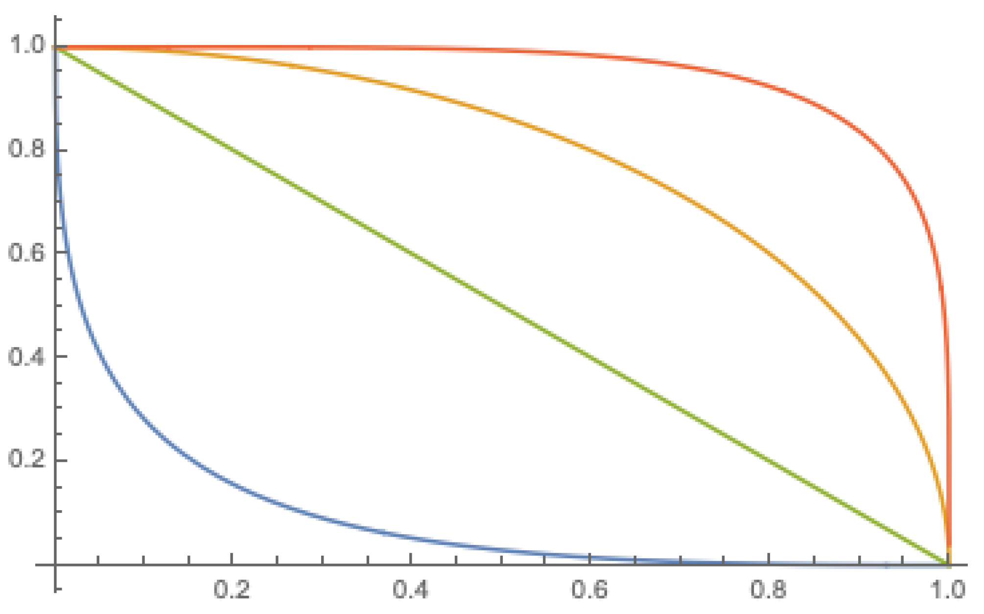
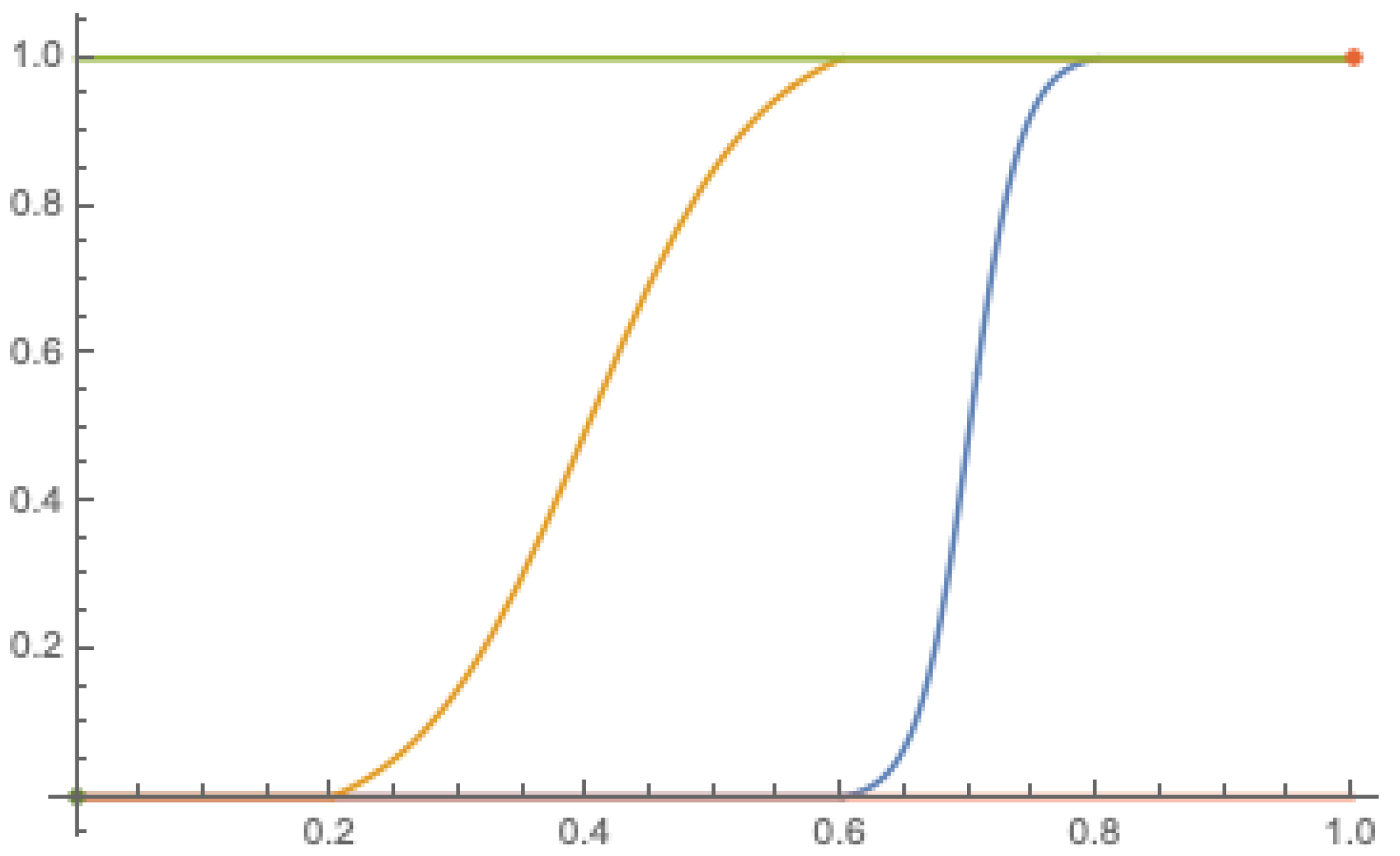
Example 3.

For the Schweizer–Sklar class of t-norms with $\lambda \in [-\infty ,\infty )$, the negation $N_{\lambda }^{SS}$ determined by the residuum ${\to }_{T_{\lambda }^{SS}}$ has the following form. For $\alpha =0$, there is $N_{\lambda }^{SS}(0)=1$, for $\alpha \ne 0$, there is

$$\begin{array}{c}{N}_{\lambda }^{SS}(\alpha )=\left\{\begin{array}{cc}0,\hfill & \lambda \in [-\infty ,0],\hfill \\ {(1-{\alpha }^{\lambda })}^{\frac{1}{\lambda }},\hfill & \lambda \in (0,\infty ),\hfill \end{array}\right.\end{array}$$

(4)

Note that for $\lambda \in (-\infty ,0)$, according to (3), we have ${(1-{\alpha }^{\lambda }+0^{\lambda })}^{\frac{1}{\lambda }}={(1-{(\frac{1}{\alpha })}^{-\lambda }+{\infty }^{-\lambda })}^{\frac{1}{\lambda }}={\infty }^{\frac{1}{\lambda }}=0^{-\frac{1}{\lambda }}=0$. Obviously, for $\lambda \in (0,\infty )$, it is sufficient to consider only one formula to express the negation, namely $N_{\lambda }^{SS}(\alpha )={(1-{\alpha }^{\lambda })}^{\frac{1}{\lambda }}$ for $\alpha \in [0,1]$. The negation $N_{\lambda }^{SS}$ is continuous, and, as a particular case, we obtain the negation $N_1^{SS}$ in the ukasiewicz algebra $L_{T_1^{SS}}$, which is well established in fuzzy logic [21,24]. Figure 3 shows four examples of negations of $N_{\lambda }^{SS}$ with positive parameter λ.

2.2. Fuzzy Sets

Let L be a complete residuated lattice, and let X be a non-empty set. A function $A:X\to [0,1]$ is called a fuzzy subsetin X. A fuzzy set A on X with $A(x)\in \{0,1\}$ for all $x\in X$ is called crisp. The symbol ∅ is used to denote the empty fuzzy set on X, i.e., $\varnothing (x)=0$ for any $x\in X$. The set of all crisp fuzzy subsets in X (i.e., the power set of X) is denoted by $\mathcal{P}(X)$. A constant fuzzy set A on X (denoted as ${\underline{\alpha }}_X$) satisfies $A(x)=\alpha$ for any $x\in X$, where $\alpha \in [0,1]$. The sets $\mathrm{Supp}(A)=\{x\mid x\in X$and$A(x)>0\}$ and $\mathrm{Core}(A)=\{x\mid x\in X$and$A(x)=1\}$ are called the support and the core of a fuzzy subset A in X, respectively. A fuzzy subset A in X is called normal if $\mathrm{Core}(A)\ne \varnothing$. The elementary operations as the union, intersection, scalar multiplication for fuzzy subsets in X are defined as follows:

$$\begin{array}{cc}\hfill (A\cup B)(x)& =A(x)\vee B(x)\hfill \\ \hfill (A\cap B)(x)& =A(x)\wedge B(x)\hfill \\ \hfill (\alpha \otimes A)(x)& =\alpha \otimes A(x)\hfill \end{array}$$

for $A,B\in \mathcal{F}(X)$ and $\alpha \in [0,1]$.

Let $X,Y$ be non-empty sets. A fuzzy subset K in $X\times Y$ is called (binary) fuzzy relation. We say that

(i)

K is normal in the second component if for any $y\in Y$ there is $x\in X$ such that $K(x,y)=1$.

(ii)

K is normal in the first component if for any $x\in X$ there is $y\in Y$ such that $K(x,y)=1$.

The fuzzy subset $K^{-1}$ in $Y\times X$ given by $K^{-1}(y,x)=K(x,y)$ is called the inverse to K. It is easy to see that if K is normal in the second (first) component, then $K^{-1}$ is normal in the first (second) component.

2.3. Fuzzy Measure Spaces

In this part, we introduce a fuzzy measure on an algebra of sets. For details, we refer to [25,26,27]. Note that fuzzy measures may also be introduced for fuzzy subsets, that is, on algebra of fuzzy sets [28], but it is rather difficult to calculate fuzzy integrals that use such type of fuzzy measures. Therefore, the practical use of integral transforms motivated us to restrict ourselves to algebras of sets. We use $X\backslash A$ to denote the complement of A in X, where A is a subset (crisp fuzzy subset) of X.

Definition 1.

Let X be a non-empty set. A subset $\mathcal{A}$ of $\mathcal{P}(X)$ is an algebra of sets on X provided that:

(i) 

$X\in \mathcal{A}$;

(ii) 

If $A\in \mathcal{A}$, then $X\backslash A\in \mathcal{A}$;

(ii) 

If $A,B\in \mathcal{A}$, then $A\cup B\in \mathcal{A}$.

A pair $(X,\mathcal{A})$ is called a measurable space on X, provided that $\mathcal{A}$ is an algebra of sets on X.

It is easy to see that if $\mathcal{A}$ is an algebra of sets, then the intersection of finite number of sets belongs to $\mathcal{A}$. Let $(X,\mathcal{A})$ be a measurable space, and $A\in \mathcal{P}(X)$. We say that A is $\mathcal{A}$-measurable if $A\in \mathcal{A}$. Obviously, the sets $\{\varnothing ,X\}$ and $\mathcal{P}(X)$ are algebras of sets on X. If $\mathcal{B}\subseteq \mathcal{P}(X)$, then the least algebra of sets containing $\mathcal{B}$ is denoted as $\mathrm{alg}(\mathcal{B})$. Note that $\mathrm{alg}(\mathcal{B})$ can be constructed from the elements of $\mathcal{B}$ as the set consisting of all finite unions applied on the set of all finite intersections over the elements of $\mathcal{B}$ and their complements.

Example 4.

Let L be a residuated lattice, and $\mathcal{L}=\left\{\right[0,\alpha ]\mid \alpha \in [0,1\left]\right\}$, where $[0,0]=\left\{0\right\}$ is a hybrid interval. Obviously, $\mathcal{L}\subset \mathcal{P}([0,1])$, and $\mathrm{alg}(\mathcal{L})$ is an algebra of sets on L, which differs from $\mathcal{P}([0,1])$. Indeed, for example, there is $[\alpha ,1]\notin \mathrm{alg}(\mathcal{L})$ for any $\alpha \in (0,1]$.

The following two definitions introduce fuzzy and complementary fuzzy measures. Note that complementary fuzzy measures and fuzzy integrals based on them were introduced in [29] to define models of fuzzy quantifiers as “no”, “little”, “few”, etc.

Definition 2.

A function $\mu :\mathcal{A}\to [0,1]$ is called a fuzzy measure on a measurable space $(X,\mathcal{A})$ if:

(i) 

$\mu (\varnothing )=0$ and $\mu (X)=1$;

(ii) 

If $A,B\in \mathcal{A}$ such that $A\subseteq B$, then $\mu (A)\le \mu (B)$.

A triplet $(X,\mathcal{A},\mu )$ is called a fuzzy measure space whenever $(X,\mathcal{A})$ is a measurable space and μ is a fuzzy measure on $(X,\mathcal{A})$.

It should be noted that the term “fuzzy measure” was introduced by Sugeno in [25], but in the literature equivalent names can be found for $\mu$, such as a capacity or a non-additive measure (see [27]). The following lemma shows how to determine a new fuzzy measure from a given fuzzy measure using a suitable function.

Lemma 1.

Let μ be a fuzzy measure on $(X,\mathcal{A})$, and let $\phi :[0,1]\to [0,1]$ be a monotonically non-decreasing function with $\phi (0)=0$ and $\phi (1)=1$. Then the function ${\mu }_{\phi }:\mathcal{A}\to [0,1]$ given by ${\mu }_{\phi }(A)=\phi (\mu (A))$ for any $A\in \mathcal{A}$ is a fuzzy measure on $(X,\mathcal{A})$.

Proof. 

The properties of the fuzzy measure for the function ${\mu }_{\phi }$ immediately follow from the monotonicity of $\phi$ and the conditions $\phi (0)=0$ and $\phi (1)=1$.    □

Definition 3.

A function $\nu :\mathcal{A}\to [0,1]$ is called a complementary fuzzy measure on a measurable space $(X,\mathcal{A})$ if:

(i) 

$\nu (\varnothing )=1$ and $\nu (X)=0$;

(ii) 

If $A,B\in \mathcal{A}$ such that $A\subseteq B$, then $\nu (A)\ge \nu (B)$.

A triplet $(X,\mathcal{A},\nu )$ is called a complementary fuzzy measure space whenever $(X,\mathcal{A})$ is a measurable space and ν is a complementary fuzzy measure on $(X,\mathcal{A})$.

The following lemma shows two ways in which a complementary fuzzy measure can be introduced from a fuzzy measure.

Lemma 2.

Let μ be a fuzzy measure on $(X,\mathcal{A})$, and let N be a negation on $[0,1]$. Then a function $\nu :\mathcal{A}\to [0,1]$ given by $\nu (A)={\mu }^c(A)=\mu (X\backslash A)$ or $\nu (A)={\mu }^N(A)=N(\mu (A))$ for any $A\in \mathcal{A}$ is a complementary fuzzy measure.

Proof. 

Obvious.    □

A dual lemma can be formulated for complementary fuzzy measures, from which the fuzzy measures can be determined by negation or set complement. Using Lemmas 1 and 2, one can introduce a broad class of fuzzy and complementary fuzzy measures. In addition to the previous two types of fuzzy measures (i.e., ${\mu }^c$ and ${\mu }^N$), we will use the so-called conjugate fuzzy measure to a given fuzzy measure.

Definition 4.

Let μ be a fuzzy measure on $(X,\mathcal{A})$, and let N be a negation on $[0,1]$. A function ${\mu }_N^c:\mathcal{A}\to [0,1]$ given by ${\mu }_N^c(A)={\mu }^N\circ {\mu }^c(A)=N(\mu (X\backslash A))$ for any $A\in \mathcal{A}$ is called a N-conjugate fuzzy measure to μ.

Note that conjugate fuzzy measures were introduced in [30] to define a type of Sugeno integral based on the residuum operation. In this case, the authors restricted themselves to the negation $N_1^{SS}$ in the ukasiewicz algebra (see Example 3). Similarly, one can introduce a N-conjugate complementary fuzzy measure. Since we deal with finite sets of pixels in image processing, the following examples present fuzzy measures defined over finite measurable spaces.

Example 5.

Let $(X,\mathcal{A})$ be a finite measurable space, that is, $X=\{x_1,\cdots ,x_n\}$. The least and thehighestfuzzy measure on $(X,\mathcal{A})$ is given by

$${\mu }^{\perp }(A)=\left\{\begin{array}{cc}0,\hfill & A\ne X,\hfill \\ 1,\hfill & \mathrm{otherwise},\hfill \end{array}\right.\mathrm{and}{\mu }^{\top }(A)=\left\{\begin{array}{cc}0,\hfill & A=\varnothing ,\hfill \\ 1,\hfill & \mathrm{otherwise},\hfill \end{array}\right.$$

(5)

for any $A\in \mathcal{A}$, respectively.

Example 6.

A relative fuzzy measure ${\mu }^r$ on $(X,\mathcal{A})$ is given as

$${\mu }^r(A)=\frac{\#A}{\#X}$$

for all $A\in \mathcal{A}$, where $\#A$ and $\#X$ denote the number of elements in A and X, respectively.

By Lemma 1, the relative fuzzy measure ${\mu }^r$ can be modified by a non-decreasing function $\phi$ with $\phi (0)=0$ and $\phi (1)=1$ to obtain a fuzzy measure ${\mu }_{\phi }^r$. In the following example, we introduce a class of functions $\phi$ that determines a class of fuzzy measures from the relative fuzzy measure, which corrects the class of functions $\phi$ presented in [8].

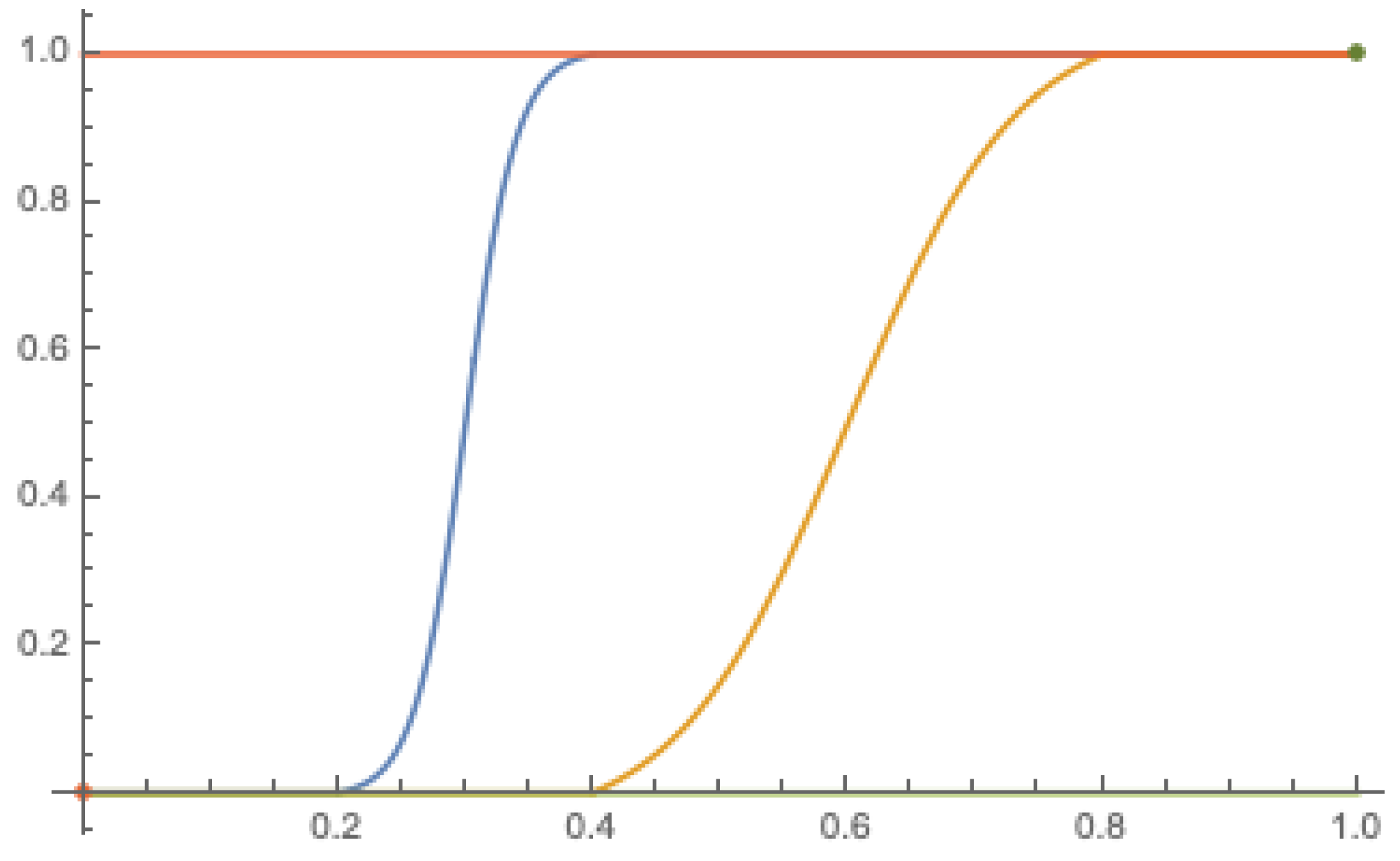
Example 7.

Let $0\le \ell \le u\le 1$ and $0<p$ be a natural number. Define ${\psi }_{\ell ,u}^p,{\phi }_{\ell ,u}^p:[0,1]\to [0,1]$ as follows:

$$\begin{array}{c}\hfill {\psi }_{\ell ,u}^p(x)=\left\{\begin{array}{cc}0,\hfill & x=0\mathrm{or}x<\ell ,\hfill \\ \frac{e^{p\left(2\frac{x-\ell }{u-\ell }-1\right)}}{e^{p\left(2\frac{x-\ell }{u-\ell }-1\right)}+1},\hfill & \ell <x\le u,\hfill \\ 1,\hfill & x=1\mathrm{or}u<x,\hfill \end{array}\right.\end{array}$$

(6)

and

$$\begin{array}{c}{\phi }_{l,u}^p(x)=\left\{\begin{array}{cc}\frac{{\psi }_{l,u}^p(x)(e^p+1)-1}{e^p-1},\hfill & l<x\le u,\hfill \\ {\psi }_{l,u}^p(x),\hfill & \mathrm{otherwise}.\hfill \end{array}\right.\end{array}$$

(7)

It could be simply verified that for $\ell <u$, ${\phi }_{\ell ,u}^p(x)$ modifies ${\psi }_{\ell ,u}^p(x)$ to obtain a continuous function on $[0,1]$. For $\ell =u$, however, ${\phi }_{\ell ,u}^p(x)$ achieves only two values 0 and 1 with the jump at the point $x=\ell$. For example, if $\ell =u=0$, then ${\phi }_{0,0}^p(x)={\psi }_{0,0}^p(0)=0$ and ${\phi }_{0,0}^p(x)={\psi }_{0,0}^p(x)=1$ for $x>0$. Examples of the function ${\phi }_{\ell ,u}^p$ for the parameters $(\ell ,u,p)\in \{(0,0,1),(0.2,0.4,5),(0.4,0.8,3),(1,1,1)\}$ are shown in Figure 4.

The function ${\phi }_{\ell ,u}^p$ obviously satisfies the assumptions of Lemma 1, so it can be used to modify any fuzzy measure. Hence, we can introduce a class of fuzzy measures on $(X,\mathcal{A})$ derived from the relative fuzzy measure ${\mu }^r$ introduced in Example 6 as follows:

$$\begin{array}{c}{\mathcal{M}}^r=\{{\mu }_{{\phi }_{\ell ,u}^p}^r\mid \ell ,u\in [0,1],\ell \le u,p\in \mathbb{N},p>0\}.\end{array}$$

(8)

It is easy to see that ${\mu }^{\perp }={\mu }_{{\phi }_{0,0}^1}^r$, ${\mu }^{\top }={\mu }_{{\phi }_{1,1}^1}^r$ and ${\mu }^r={\mu }_{{\phi }_{0,1}^1}^r$.

Example 8.

By ${\phi }_{\ell ,u}^p$ from the previous example, we can introduce two additional functions through which the complementary and conjugate fuzzy measures can be determined from the relative fuzzy measure. Let N be a negation on $[0,1]$ and define ${\phi }_{\ell ,u}^{p,c},{\phi }_{\ell ,u}^{p,N}:[0,1]\to [0,1]$ as follows:

$$\begin{array}{c}{\phi }_{\ell ,u}^{p,c}(x)={\phi }_{\ell ,u}^p(1-x)\mathrm{and}{\phi }_{\ell ,u}^{p,N}(x)=N({\phi }_{\ell ,u}^p(x)),\end{array}$$

(9)

for any $x\in [0,1]$. By Lemma 2, it is easy to check that ${\mu }_{{\phi }_{\ell ,u}^{p,c}}^r$ and ${\mu }_{{\phi }_{\ell ,u}^{p,N}}^r$ are complementary fuzzy measures on $(X,\mathcal{A})$. Define ${\phi }_{\ell ,u}^{p,c,N}={\phi }_{\ell ,u}^{p,N}\circ {\phi }_{\ell ,u}^{p,c}$, then ${\mu }_{{\phi }_{\ell ,u}^{p,c,N}}^r$ is an N-conjugate fuzzy measure to a fuzzy measure ${\mu }_{{\phi }_{\ell ,u}^p}^r$ on $(X,\mathcal{A})$. In Figure 5, we display the functions ${\phi }_{\ell ,u}^{p,c,N}$ for the same parameters as in Example 7 and $N(\alpha )=1-\alpha$ for $\alpha \in [0,1]$ (i.e., the negation in the ukasiewicz algebra). One can see that the conjugate fuzzy measure to ${\mu }^{\perp }$ (${\mu }^{\top }$) is ${\mu }^{\top }$ (${\mu }^{\perp }$); it is sufficient to compare the green (orange) functions in Figure 4 and Figure 5). Fuzzy measures ${\mu }_{{\phi }_{0,1}^p}^r$ are self-conjugate, which immediately follows from ${\phi }_{0,1}^p={\phi }_{0,1}^{p,c,N}$.

Remark 1.

It is easy to see that all fuzzy measures (and similarly complementary and conjugate fuzzy measures) in the above examples are cardinality invariant, that is, for any sets A and B such that $\#A=\#B$, it holds that $\mu (A)=\mu (B)$. Fuzzy measures invariant with respect to the cardinality of the set are referred to as symmetric fuzzy measures.

2.4. Multiplication and Residuum-Based Sugeno-like Fuzzy Integrals

In what follows, the integrated functions are fuzzy sets on X and are denoted by f, g, etc. First, we recall the definition of the multiplication-based fuzzy integral introduced in [28,30].

Definition 5.

Let $(X,\mathcal{A},\mu )$ be a fuzzy measure space, and let $f:X\to [0,1]$. The⊗-fuzzy integral of f on Xis given by

$$\begin{array}{c}{\int }^{\otimes }fd\mu =\underset{\begin{array}{c}A\in \mathcal{A}\end{array}}{\bigvee }\mu (A)\otimes \left(\underset{x\in A}{\bigwedge }f(x)\right).\end{array}$$

(10)

Let $(X,\mathcal{A},\mu )$ be a fuzzy measure space. We say that a function $f:X\to L$ is measurable, if $\{x_i\mid f(x_i)\ge \alpha \}\in \mathcal{A}$ for any $\alpha \in [0,1]$. For measurable functions, the ⊗-fuzzy integral can be calculated as follows (see, Theorem 3.2 in [1]).

Theorem 1.

Let $(X,\mathcal{A},\mu )$ be a fuzzy measure space, and let $f:X\to [0,1]$ be a measurable function. Then

$$\begin{array}{c}{\int }^{\otimes }fd\mu =\underset{\begin{array}{c}\alpha \in [0,1]\end{array}}{\bigvee }\left(\alpha \otimes \mu (\{x\in X\mid f(x)\ge \alpha \})\right).\end{array}$$

(11)

The following corollary provides a simple computational formula for the ⊗-fuzzy integral of measurable functions defined on a finite set $X=\{x_1,\cdots ,x_n\}$. Denote $\left[n\right]=\{1,\cdots ,n\}$.

Corollary 1.

Let $(X,\mathcal{A},\mu )$ be a finite fuzzy measure space, that is, $X=\{x_1,\cdots ,x_n\}$, and let $f:X\to [0,1]$ be measurable. Then

$$\begin{array}{c}{\int }^{\otimes }fd\mu =\underset{i\in \left[n\right]}{\bigvee }{f}_{\sigma (i)}\otimes {\mu }_i,\end{array}$$

(12)

where σ is a permutation on $\left[n\right]$ such that $f_{\sigma (1)}\le f_{\sigma (2)}\le \cdots \le f_{\sigma (n)}$, where $f_{\sigma (i)}=f(x_{\sigma (i)})$ for $i\in \left[n\right]$ and ${\mu }_i=\mu (\{x_{\sigma (i)},\cdots ,x_{\sigma (n)}\})$.

Proof. 

It immediately follows from Theorem 1, where we restrict the calculation from $\alpha \in [0,1]$ to $\alpha \in \{f_{\sigma (1)},\cdots ,f_{\sigma (n)}\}$. Indeed, for $\alpha =0$ or $f_{\sigma (n)}<\alpha \le 1$, we trivially obtain $\alpha \otimes \mu (\{x\in X\mid f(x)\ge \alpha \})=0$. If $f_{\sigma (i-1)}<\alpha \le f_{\sigma (i)}$ for $i\in \left[n\right]$ (we put $f_{\sigma (0)}=0$), then

$$\begin{array}{c}\alpha \otimes \mu (\{x\in X\mid f(x)\ge \alpha \})=\alpha \otimes {\mu }_i\le f_{\sigma (i)}\otimes {\mu }_i,\end{array}$$

where we used the fact that the multiplication is non-decreasing in both variables. Hence, we find that

$$\begin{array}{c}\underset{\begin{array}{c}\alpha \in [0,1]\end{array}}{\bigvee }\left(\alpha \otimes \mu (\{x\in X\mid f(x)\ge \alpha \})\right)\le \underset{i\in \left[n\right]}{\bigvee }{f}_{\sigma (i)}\otimes {\mu }_i.\end{array}$$

Since the opposite inequality is trivially true, we obtain the desired equality.    □

Note that, if $\mathcal{A}=\mathcal{P}(X)$, then any function $f:X\to [0,1]$ is measurable, and thus its ⊗-fuzzy integral can be calculated using formula (12). Calculation by Formula (12) can even be simplified for symmetric fuzzy measures, because it is sufficient to define ${\mu }_i=\mu (\{x_i,\cdots ,x_n\})$ for any $i\in \left[n\right]$.

Now, we introduce a modified version of the original definition of residuum-based fuzzy integral presented in [29].

Definition 6.

Let $(X,\mathcal{A},\nu )$ be a complementary fuzzy measure space, and let $f:X\to L$. The →-fuzzy integral of f on X is given by

$$\begin{array}{c}{\int }^{\to }fd\nu =\underset{\begin{array}{c}A\in \mathcal{A}\end{array}}{\bigwedge }\left(\underset{x\in A}{\bigwedge }f(x)\right)\to \nu (A).\end{array}$$

(13)

Note that a residuum-based fuzzy integral was also proposed by Dubois, Prade, and Rico in [30] under the name desintegral for reasoning with a decreasing evaluation scale. A comparison of both fuzzy integrals can be found in [31]. Similarly to the multiplication-based fuzzy integral, for measurable functions, we get a more pleasant computational formula.

Theorem 2.

Let $(X,\mathcal{A},\nu )$ be a complementary fuzzy measure space, and let $f:X\to [0,1]$ be a measurable function. Then

$$\begin{array}{c}{\int }^{\to }fd\nu =\underset{\begin{array}{c}\alpha \in [0,1]\end{array}}{\bigwedge }\left(\alpha \to \nu (\{x\in X\mid f(x)\ge \alpha \})\right).\end{array}$$

(14)

Proof. 

Denote $L_{\alpha }=\{x\in [0,1]\mid x\ge \alpha \}$ for any $\alpha \in [0,1]$. It is easy to see that

$$\begin{array}{c}{f}^{-1}(L_a)=\{x\in X\mid f(x)\in L_a\}=\{x\in X\mid f(x)\ge \alpha \}.\end{array}$$

Put

$$\begin{array}{cc}\hfill K& =\underset{\begin{array}{c}A\in \mathcal{A}\end{array}}{\bigwedge }\left(\left(\underset{x\in A}{\bigwedge }f(x)\right)\to \nu (A)\right)\hfill \\ \hfill L& =\underset{\begin{array}{c}\alpha \in [0,1]\end{array}}{\bigwedge }\left(\alpha \to \nu \left(f^{-1}(L_{\alpha })\right)\right).\hfill \end{array}$$

First, we show that $K\ge L$. Define ${\lambda }_f:\mathcal{A}\to [0,1]$ by ${\lambda }_f(A)={\bigwedge }_{x\in A}f(x)$. Obviously, we have $A\subseteq f^{-1}(L_{{\lambda }_f(A)})$, and thus $\nu (f^{-1}(L_{{\lambda }_f(A)}))\le \nu (A)$ by (ii) of Definition 3. Since ${\lambda }_f(\mathcal{A})\subseteq [0,1]$, we get

$$\begin{array}{c}K=\underset{A\in \mathcal{A}}{\bigwedge }({\lambda }_f(A)\to \nu (A))\ge \underset{A\in \mathcal{A}}{\bigwedge }({\lambda }_f(A)\to \nu (f^{-1}(L_{{\lambda }_f(A)})))\ge L,\end{array}$$

where we used the fact that the residuum is non-decreasing in its second variable.

Furthermore, we show that $K\le L$. Define ${\varrho }_f:[0,1]\to \mathcal{A}$ by ${\varrho }_f(\alpha )=f^{-1}(L_{\alpha })$. Since f is measurable, the function ${\varrho }_f$ is well defined. Obviously, we have ${\bigwedge }_{x\in {\varrho }_f(\alpha )}f(x)\ge \alpha$ for any $\alpha \in [0,1]$ and ${\varrho }_f([0,1])\subseteq \mathcal{A}$. Hence, we obtain

$$\begin{array}{c}K\le \underset{\alpha \in [0,1]}{\bigwedge }\left(\left(\underset{x\in {\varrho }_f(\alpha )}{\bigwedge }f(x)\right)\to \nu ({\varrho }_f(\alpha ))\right)\le \underset{\alpha \in [0,1]}{\bigwedge }(\alpha \to \nu (f^{-1}(L_{\alpha }))=L,\end{array}$$

where we used the fact that the residuum is non-increasing in its first variable. Hence, we obtain $K=L$, and the proof is completed.    □

As a corollary, we get a simple computational formula for measurable functions defined on finite set $X=\{x_1,\cdots ,x_n\}$.

Corollary 2.

Let $(X,\mathcal{A},\nu )$ be a finite complementary fuzzy measure space, that is, $X=\{x_1,\cdots ,x_n\}$, and let $f:X\to [0,1]$ be measurable. Then

$$\begin{array}{c}{\int }^{\to }fd\nu =\underset{i\in \left[n\right]}{\bigwedge }{f}_{\sigma (i)}\to {\nu }_i,\end{array}$$

(15)

where σ is a permutation on $\left[n\right]$ such that $f_{\sigma (1)}\le f_{\sigma (2)}\le \cdots \le f_{\sigma (n)}$, where $f_{\sigma (i)}=f(x_{\sigma (i)})$ for $i\in \left[n\right]$, and ${\nu }_i=\nu (\{x_{\sigma (i)},\cdots ,x_{\sigma (n)}\})$.

Proof. 

Analogously to the proof of Corollary 1, for $\alpha =0$ and $f_{\sigma (n)}<\alpha \le 1$, we find that $\alpha \to \nu (\{x\in X\mid f(x)\ge \alpha \})=\alpha \to \nu (\varnothing )=\alpha \to 1=1$. If $f_{\sigma (i-1)}<\alpha \le f_{\sigma (i)}$ for $i\in \left[n\right]$ (we put $f_{\sigma (0)}=0$), then

$$\begin{array}{c}\alpha \to \nu (\{x\in X\mid f(x)\ge \alpha \})=\alpha \to {\nu }_i\ge f_{\sigma (i)}\to {\nu }_i,\end{array}$$

where we used the fact that the residuum is non-increasing in its first variable. Hence, we get

$$\begin{array}{c}\underset{\begin{array}{c}\alpha \in [0,1]\end{array}}{\bigwedge }\left(\alpha \to \nu (\{x\in X\mid f(x)\ge \alpha \})\right)\ge \underset{i\in \left[n\right]}{\bigwedge }{f}_{\sigma (i)}\to {\nu }_i.\end{array}$$

Since the opposite inequality is trivially true, we obtain the desired equality.    □

It should be noted that there is a relationship between both types of fuzzy integrals under specific conditions on the residuated lattice (see [31]). For more information on both types of fuzzy integrals, we refer to [1,16,28,29].

3. Lattice Integral Transforms

In this part, we introduce two types of integral transforms for lattice-valued functions related to multiplication and residuum-based fuzzy integrals. As with the classical integral transform, the key concept in our lattice integral transform theory is an integral kernel. The following definition was provided in [17].

Definition 7.

A fuzzy relation $K:X\times Y\to L$ that is normal in the second argument is said to be an integral kernel.

The next definition generalizes the upper and lower F-transforms and unifies the definitions of lattice integral transforms mentioned in the Introduction (see [1]).

Definition 8.

Let $(X,\mathcal{A},\mu )$ be a fuzzy measure space, let $K:X\times Y\to [0,1]$ be an integral kernel, and let $\star \in \{\otimes ,\to \}$. A function $F_{(K,\mu )}^{\star }:\mathcal{F}(X)\to \mathcal{F}(Y)$ defined by

$$\begin{array}{c}{F}_{(K,\mu )}^{\star }(f)(y)={\int }^{\otimes }K(x,y)\star f(x)d\mu \end{array}$$

(16)

is called a $(K,\mu ,\star )$-lattice integral transform.

The elementary properties of the integral transform for lattice-valued functions can be presented in the following theorem.

Theorem 3.

Let $\star \in \{\otimes ,\to \}$, and put $F^{\star }=F_{(K,\mu )}^{\star }$. For any $f,g\in \mathcal{F}(X)$ and $\alpha \in [0,1]$, we have

(i) 

$F^{\star }(f)\le F^{\star }(g)$ if $f\le g$;

(ii) 

$F^{\star }(f\cap g)\le F^{\star }(f)\wedge F^{\star }(g)$;

(iii) 

$F^{\star }(f)\vee F^{\star }(g)\le F^{\star }(f\cup g)$;

(iv) 

$\alpha \otimes F^{\star }(f)\le F^{\star }(\alpha \otimes f)$;

(v) 

$F^{\star }(\alpha \to f)\le \alpha \to F^{\star }(f)$.

Proof. 

See [1].    □

The next theorem introduced without proof in [17] (see also [8]) shows conditions under which a constant function (fuzzy set) ${\underline{\alpha }}_X$ is transformed into a constant function ${\underline{\alpha }}_Y$, that is, $F_{(K,\mu )}^{\star }({\underline{\alpha }}_X)={\underline{\alpha }}_Y$. For an integral kernel K on $X\times Y$ and $y\in Y$, we use $K_y$ to denote a fuzzy subset of X given by $K_y(x)=K(x,y)$ for any $x\in X$. Recall that $\mathrm{Core}(K_y)\ne \varnothing$ follows from the definition of the integral kernel.

Theorem 4.

Let $(X,\mathcal{A},\mu )$ be a fuzzy measure space, let K be an integral kernel, and let $\alpha \in [0,1]$.

(i) 

If for any $y\in Y$ there exists $A_y\in \mathcal{A}$ such that $A_y\subseteq \mathrm{Core}(K_y)$ and $\mu (A_y)=1$, then $F_{(K,\mu )}^{\otimes }({\underline{\alpha }}_X)={\underline{\alpha }}_Y$.

(ii) 

If for any $y\in Y$ and for any $A\in \mathcal{A}$ with $A\subseteq X\backslash \mathrm{Core}(K_y)$ it holds that $\mu (A)\le \alpha$, then $F_{(K,\mu )}^{\to }({\underline{\alpha }}_X)={\underline{\alpha }}_Y$.

Proof. 

(i) Let $\alpha \in [0,1]$ and $y\in Y$. By the assumption of (i), we assume that there is $A_y\subseteq \mathrm{Core}(K_y)$ such that $\mu (A_y)=1$. Then

$$\begin{array}{cc}\hfill F_{(K,\mu )}^{\otimes }({\underline{\alpha }}_X)(y)& ={\int }^{\otimes }K(x,y)\otimes {\underline{\alpha }}_X(x)d\mu \hfill \\ \hfill & =\underset{\begin{array}{c}A\in \mathcal{A}\end{array}}{\bigvee }(\mu (A)\otimes \underset{x\in A}{\bigwedge }(K(x,y)\otimes {\underline{\alpha }}_X(x))\hfill \\ \hfill & =\underset{\begin{array}{c}A\in \mathcal{A}\end{array}}{\bigvee }(\mu (A)\otimes \underset{x\in A}{\bigwedge }(K(x,y)\otimes \alpha )\hfill \\ \hfill & \ge \mu (A_y)\otimes \underset{x\in A_y}{\bigwedge }(K(x,y)\otimes \alpha )=1\otimes \alpha =\alpha .\hfill \end{array}$$

On the other hand, it is trivially true that $\mu (A)\otimes {\bigwedge }_{x\in A}(K(x,y)\otimes \alpha )\le \alpha$ for any $A\in \mathcal{A}$. Therefore, we find $F_{(K,\mu )}^{\otimes }({\underline{\alpha }}_X)(y)\le \alpha$, which proves the desired equality.

(ii) Let $\alpha \in [0,1]$ and $y\in Y$. By the assumption of (ii), for any $A\in \mathcal{A}$ such that $A\subseteq X\backslash \mathrm{Core}(K_y)$, we have $\mu (A)\le \alpha$. Since $\mathrm{Core}(K_y)\ne \varnothing$, we get $X⊈X\backslash \mathrm{Core}(K_y)$. Then

$$\begin{array}{cc}\hfill F_{(K,\mu )}^{\to }({\underline{\alpha }}_X)(y)& ={\int }^{\otimes }K(x,y)\to {\underline{\alpha }}_X(x)d\mu \hfill \\ \hfill & =\underset{\begin{array}{c}A\in \mathcal{A}\\ A⊈X\backslash \mathrm{Core}(K_y)\end{array}}{\bigvee }(\mu (A)\otimes \underset{x\in A}{\bigwedge }(K(x,y)\to \alpha ))\vee \hfill \\ \hfill & \underset{\begin{array}{c}A\in \mathcal{A}\\ A\subseteq X\backslash \mathrm{Core}(K_y)\end{array}}{\bigvee }(\mu (A)\otimes \underset{x\in A}{\bigwedge }(K(x,y)\to \alpha ))\hfill \\ \hfill & \le \underset{\begin{array}{c}A\in \mathcal{A}\\ A⊈X\backslash \mathrm{Core}(K_y)\end{array}}{\bigvee }(\alpha \otimes \mu (A))\vee \underset{\begin{array}{c}A\in \mathcal{A}\\ A\subseteq X\backslash \mathrm{Core}(K_y)\end{array}}{\bigvee }\mu (A)\hfill \\ \hfill & =\alpha \otimes \underset{\begin{array}{c}A\in \mathcal{A}\\ A⊈X\backslash \mathrm{Core}(K_y)\end{array}}{\bigvee }\mu (A)=\alpha \otimes \mu (X)=\alpha ,\hfill \end{array}$$

where we used the distributivity of ⊗ over ⋁, the equality

$$\begin{array}{c}\underset{x\in A}{\bigwedge }(K(x,y)\to \alpha ))=\alpha \end{array}$$

for any $A⊈X\backslash \mathrm{Core}(K_y)$, which follows from $K(x,y)=1$ for some $x\in A$, $1\to \alpha =\alpha$, and $\beta \to \alpha \ge \alpha$ for any $\beta \in [0,1]$, and the assumption stating that $\mu (A)\le \alpha$ for any $A\in \mathcal{A}$, such that $A\subseteq X\backslash \mathrm{Core}(K_y)$. On the contrary, we have

$$\begin{array}{c}{F}_{(K,\mu )}^{\to }({\underline{\alpha }}_X)(y)\ge \underset{x\in X}{\bigwedge }K(x,y)\to {\underline{\alpha }}_X(x)=\underset{x\in X}{\bigwedge }(K(x,y)\to \alpha )=\alpha ,\end{array}$$

where we used the same arguments as above, which proves the desired equality.    □

It is worth noting that the standard real-valued F-transforms as well as lower and upper lattice-valued F-transforms preserve constant functions; therefore, it seems to be reasonable to assume that integral kernels and fuzzy measures as the parameters of the integral transforms satisfy the conditions under which the constant functions are preserved.

Example 9.

Let $(X,\mathcal{A})$ be a measurable space with $X=\{x_1,\cdots ,x_n\}$ and $\mathcal{A}=\mathcal{P}(X)$, and let ${\mathcal{M}}^r$ be the class of fuzzy measures on $(X,\mathcal{A})$ introduced in Example 7. Let $K:X\times Y\to [0,1]$ be an integral kernel, where $Y=\{y_1,\cdots ,y_m\}$ and put $u=min\{\#\mathrm{Core}(K_{y_j})\mid y_j\in Y\}/n$. Then the class

$$\begin{array}{c}{\mathcal{M}}_u^r=\{{\mu }_{{\phi }_{\ell ,u}^p}^r\mid \ell \in [0,1],\ell \le u,p\in \mathbb{N},p>0\}\end{array}$$

(17)

consists of all fuzzy measures, for which the $(K,\mu ,\otimes )$-integral transform preserves constant functions. Indeed, we trivially have $\mathrm{Core}(K_{y_j})\in \mathcal{A}$ for any $y_j\in Y$. By the definition of u, we find that for any $y_j\in Y$ it holds

$${\mu }_{{\phi }_{\ell ,u}^p}^r(\mathrm{Core}(K_{y_j}))={\phi }_{\ell ,u}^p(\#\mathrm{Core}(K_{y_j})/n)=1$$

for any $\ell \le u$ and $p>0$, since $u\le \#\mathrm{Core}(K_{y_j})/n$. Therefore, the assumption in (i) of Theorem 4 is satisfied, and thus the $(K,\mu ,\otimes )$-integral transform preserves constant functions for any $\mu \in {\mathcal{M}}_u^r$.

In addition, the class

$$\begin{array}{c}{\mathcal{M}}_u^{r,c,N}=\{{\mu }_{{\phi }_{\ell ,u}^{p,c,N}}^r\mid \ell \in [0,1],\ell \le u,p\in \mathbb{N},p>0\}\end{array}$$

(18)

consists of all fuzzy measures (N-conjugate fuzzy measures to fuzzy measures from ${\mathcal{M}}_u^r$), for which the $(K,\mu ,\to )$-integral transform preserves constant functions. Indeed, let us show that an N-conjugate fuzzy measure to $\mu \in {\mathcal{M}}_u^r$ satisfies the assumption in (ii) of Theorem 4. Let $\mu ={\phi }_{\ell ,u}^p\circ {\mu }^r$. Recall that ${\mu }_N^c(A)=N(\mu (X\backslash A))$ for any $A\in \mathcal{A}$. Let $y_j\in Y$, $B\in \mathcal{A}$ be arbitrary, such that $B\subseteq X\backslash \mathrm{Core}(K_{y_j})$, and put $s=\#B$. Since $\#\mathrm{Core}(K_{y_j})/n\ge u$, we find that $s=\#B\le \#(X\backslash \mathrm{Core}(K_{y_j}))\le n-n·u$; therefore, ${\mu }^r(X\backslash B)=\#(X\backslash B)/n=(n-s)/n=1-s/n\ge 1-(1-u)=u$. Since N is a non-increasing function and ${\phi }_{l,u}^p$ is a non-decreasing function, we get

$$\begin{array}{c}{\mu }_N^c(B)=N(\mu (X\backslash B))=N({\phi }_{l,u}^p({\mu }^r(X\backslash B)))\le N({\phi }_{l,u}^p(u))=N(1)=0,\end{array}$$

where ${\phi }_{l,u}^p(u)=1$ follows from the definition of ${\phi }_{l,u}^p$. Hence, the assumption in (ii) of Theorem 4 is satisfied, and thus the $(K,\mu ,\to )$-integral transform preserves arbitrary constant functions for any fuzzy measure from ${\mathcal{M}}_u^{r,c,N}$.

The next definition introduces a “reverse” alternative to the lattice integral transform introduced above, where the residuum-based fuzzy integral on a complementary fuzzy measure space is considered instead of the multiplication one.

Definition 9.

Let $(X,\mathcal{A},\nu )$ be a complementary fuzzy measure space, let $K:X\times Y\to L$ be an integral kernel, and let $\star \in \{\otimes ,\to \}$. A function $G_{(K,\nu )}^{\star }:\mathcal{F}(X)\to \mathcal{F}(Y)$ defined by

$$\begin{array}{c}{G}_{(K,\nu )}^{\star }(f)(y)={\int }^{\to }K(x,y)\star f(x)d\nu \end{array}$$

(19)

is called a $(K,\nu ,\star )$-reverse lattice integral transform.

We use the term “reverse lattice integral transform” to simply distinguish between both types of lattice integral transforms. The next theorem presents selected properties of the reverse lattice integral transform.

Theorem 5.

Let $\star \in \{\otimes ,\to \}$, and put $G^{\star }=G_{(K,\nu )}^{\star }$. For any $f,g\in \mathcal{F}(X)$ and $\alpha \in [0,1]$, we have

(i) 

$G^{\star }(f)\ge G^{\star }(g)$ if $f\le g$;

(ii) 

$G^{\star }(f\cap g)\ge G^{\star }(f)\vee G^{\star }(g)$;

(iii) 

$G^{\star }(f)\wedge G^{\star }(g)\ge G^{\star }(f\cup g)$;

(iv) 

$G^{\star }(\alpha \otimes f)\le \alpha \to G^{\star }(f)$;

(v) 

$G^{\star }(\alpha \to f)\ge \alpha \otimes G^{\star }(f)$.

Proof. 

See [16].    □

Similarly to Theorem 4, we are interested in sufficient conditions under which reverse lattice integral transforms ensure the reversal of constant functions, i.e., $G_{(K,\nu )}^{\otimes }({\underline{\alpha }}_X)={\underline{\neg \alpha }}_Y$, where ¬ is the standard negation defined by the residuum, i.e., $\neg \alpha =\alpha \to 0$.

Theorem 6.

Let $(X,\mathcal{A},\nu )$ be a complementary fuzzy measure, let K be an integral kernel, and let $\alpha \in [0,1]$.

(i) 

If for any $y\in Y$ there exists $A_y\in \mathcal{A}$ such that $A_y\subseteq \mathrm{Core}(K_y)$ and $\nu (A_y)=0$, then $G_{(K,\nu )}^{\otimes }({\underline{\alpha }}_X)={\underline{\neg \alpha }}_Y$;

(ii) 

If for any $y\in Y$ and for any $A\in \mathcal{A}$ with $A\subseteq X\backslash \mathrm{Core}(K_y)$ it holds that $\nu (A)\ge \neg \alpha$, then $G_{(K,\nu )}^{\to }({\underline{\alpha }}_X)={\underline{\neg \alpha }}_Y$.

Proof. 

(i) Let $y\in Y$, and ${\underline{\alpha }}_X\in \mathcal{F}(X)$. Assume that there is $A_y\subseteq \mathrm{Core}(K_y)$ such that $\nu (A_y)=0$. Then

$$\begin{array}{c}{G}_{(K,\nu )}^{\otimes }({\underline{\alpha }}_X)(y)={\int }^{\to }K(x,y)\otimes {\underline{\alpha }}_X(x)d\nu =\underset{\begin{array}{c}A\in \mathcal{A}\end{array}}{\bigwedge }\left(\underset{x\in A}{\bigwedge }(K(x,y)\otimes \alpha )\to \nu (A)\right)\\ \le \underset{x\in A_y}{\bigwedge }(1\otimes \alpha )\to 0=\alpha \to 0=\neg \alpha ={\underline{\neg \alpha }}_Y(y).\end{array}$$

On the other hand, for any $A\in \mathcal{A}$, we trivially have ${\bigwedge }_{x\in A}(K(x,y)\otimes \alpha )\to \nu (A)\ge \alpha \to 0={\underline{\neg \alpha }}_Y(y)$, where we used the monotonically non-increasing in the first argument and the monotonically non-decreasing in the second argument of residuum. Hence, we find $G_{(K,\nu )}^{\otimes }({\underline{\alpha }}_X)(y)\ge {\underline{\neg \alpha }}_Y(y)$, which proves the desired equality.

(ii) Let $y\in Y$. Since $\mathrm{Core}(K_y)\ne \varnothing$, so $X⊈X\backslash \mathrm{Core}(K_y)$. Then

$$\begin{array}{c}{G}_{(K,\nu )}^{\to }({\underline{\alpha }}_X)(y)={\int }^{\to }K(x,y)\to {\underline{\alpha }}_X(x)d\nu =\underset{\begin{array}{c}A\in \mathcal{A}\\ A\subseteq X\backslash \mathrm{Core}(K_y)\end{array}}{\bigwedge }\left(\underset{x\in A}{\bigwedge }(K(x,y)\to \alpha )\to \nu (A)\right)\\ \wedge \underset{\begin{array}{c}A\in \mathcal{A}\\ A⊈X\backslash \mathrm{Core}(K_y)\end{array}}{\bigwedge }\left(\underset{x\in A}{\bigwedge }(K(x,y)\to \alpha )\to \nu (A)\right)\ge \underset{\begin{array}{c}A\in \mathcal{A}\\ A\subseteq X\backslash \mathrm{Core}(K_y)\end{array}}{\bigwedge }(1\to \nu (A))\\ \wedge \underset{\begin{array}{c}A\in \mathcal{A}\\ A⊈X\backslash \mathrm{Core}(K_y)\end{array}}{\bigwedge }(\alpha \to \nu (A))\ge \neg \alpha \wedge (\alpha \to 0)=\neg \alpha ={\underline{\neg \alpha }}_Y(y),\end{array}$$

where we used that the residuum is monotonically non-increasing in the first component and the monotonically non-decreasing in the second component, i.e., trivially $K(x,y)\to \alpha \le 1$, therefore, $(K(x,y)\to \alpha )\to \nu (A)\ge 1\to \nu (A)=\nu (A)\ge \neg \alpha$ for $A\subseteq X\backslash \mathrm{Core}(K_y)$ by the assumption in (ii). On the contrary, we have:

$$\begin{array}{c}{G}_{(K,\nu )}^{\to }({\underline{\alpha }}_X)(y)\le \underset{x\in X}{\bigwedge }(K(x,y)\to \alpha )\to \nu (X)=\alpha \to 0=\neg \alpha ={\underline{\neg \alpha }}_Y(y),\end{array}$$

where we used the fact that $K(x,y)\to \alpha \ge \alpha$ for any $(x,y)\in X\times Y$ and $K(x,y)\to \alpha =1\to \alpha =\alpha$ for any $x\in \mathrm{Core}(K_y)$, which proves the desired equality.    □

Example 10.

From Lemma 2, we know that a complementary fuzzy measure can be introduced from a given fuzzy measure using a negation N on $[0,1]$ as ${\nu }_N(A)=N(\mu (A))$ for any $A\in \mathcal{A}$. It is easy to observe that if K is an integral kernel and μ a fuzzy measure such that (i) (or (ii)) of Theorem 4 is satisfied, then ${\nu }_N$ is a complementary fuzzy measure that satisfies (i) (or (ii)) of Theorem 6, where $N=\neg$ for case (ii). In fact, if $\mu (A_y)=1$ for some $A_y\subseteq \mathrm{Core}(K_y)$, then ${\nu }_N(A_y)=N(\mu (A_y))=N(1)=0$. Similarly, if for any $A\subseteq X\backslash \mathrm{Core}(K_y)$, we have $\mu (A)\le \alpha$, then ${\nu }_N(A)=N(\mu (A))\ge N(\alpha )=\neg \alpha$. Obviously, if $G_{(K,\nu )}^{\to }$ has to reverse an arbitrary constant function, that is, (ii) of Theorem 6 holds for any $\alpha \in [0,1]$, which is equivalent to $\nu (A)=1$ holds for any $A\in \mathcal{A}$ with $A\subseteq X\backslash \mathrm{Core}(K_y)$, then we can consider an arbitrary negation N on $[0,1]$ to get the desired reversal.

4. Application of Lattice Integral Transforms to Image Processing

In this part, we apply lattice integral transforms (LITs for short) to image processing, namely, non-linear filtering, compression/decompression and closing/opening of images. For the purpose of this paper, we restrict ourselves to grayscale images. We assume that an image h of the size $N\times M$ (the number of pixels in rows and columns) is a function $I:D\to [0,1]$, where $D=\{(i,j)\mid 1\le i\le N,1\le j\le M\}$ and the value $I(i,j)$ expresses the intensity of shades of gray from black to white for the pixel at the position $(i,j)\in D$. For simplicity, we assume that the shade of gray can be determined for any number from $[0,1]$. Since an image is a two-dimensional function, we consider lattice integral transforms from $\mathcal{F}(D_1)$ to $\mathcal{F}(D_2)$, where $D_1$ is the domain of original (input) images and $D_2$ is the domain of output images (e.g., compressed images). In the following part, we first describe in detail the way in which the lattice integral transforms are applied to the above tasks and then demonstrate them in various images. For an introduction to methods used in non-linear image processing, we refer to [32,33].

4.1. Method Description

Let $N,M,\varrho$ be natural numbers such that $\varrho$ divides N and M. Denote $n=N/\varrho$ and $m=M/\varrho$. The number $\varrho$ will be called the shift and ${\varrho }^2:1$ will express compression ratio. Denote $D=\{(i,j)\mid 1\le i\le N,1\le j\le M\}$ and $D_{\varrho }=\{(i,j)\mid 1\le i\le n,1\le j\le m\}$, where $D_{\varrho }$ provides the domain for compressed images ($\varrho >1$) or filtered images ($\varrho =1$).

Let $r,s$ be natural numbers such that $\varrho \le r\ll N$ and $\varrho \le s\ll M$, and denote $[-r,r]=\{-r,\cdots ,0,\cdots ,r\}$ and similarly for $[-s,s]$. Let $W=\{w_{i,j}\mid i\in [-r,r],j\in [-s,s]\}$ be an $(2r+1)\times (2s+1)$ matrix of values from $[0,1]$, which will be referred to as window of size $R\times S$, where $R=2r+1$ and $S=2s+1$. A window W specifies the weights assigned to pixels in the neighborhood of a corresponding pixel in the input image. In our application, we assume that $w_{00}=1$. Note that W can be viewed as a normal fuzzy relation on $[-r,r]\times [-s,s]$.

To properly process the pixels at the edges of the images, we extend D to a broader domain given as

$$\begin{array}{c}{D}_{r,s}=\{(i,j)\mid -r+1\le i\le N+r,-s+1\le j\le M+s\},\end{array}$$

and consider a function  $\widehat{}:\mathcal{F}(D)\to \mathcal{F}(D_{r,s})$ that each image $I\in \mathcal{F}(D)$ extends to an image $\widehat{I}\in \mathcal{F}(D_{r,s})$ such that $\widehat{I}(i,j)=I(i,j)$ for any $(i,j)\in D$. The extension of I for pixels from $D_{r,s}\backslash D$ can be adjusted in different ways according to the given task. For example, we can consider the following extending functions:

(a)

$\widehat{I}(i,j)=I(i,j)$, for $(i,j)\in D$, and $\widehat{I}(i,j)=1$, otherwise, which is used in dilation;

(b)

$\widehat{I}(i,j)=I(i,j)$, for $(i,j)\in D$, and $\widehat{I}(i,j)=0$, otherwise, which is used in erosion;

(c)

$\widehat{I}(i,j)=I(i^{\prime },j^{\prime })$, where

$$\begin{array}{c}{i}^{\prime }=2·max(1,min(N,i))-i\mathrm{and}{j}^{\prime }=2·max(1,min(M,j))-j.\end{array}$$

It is easy to see that $i^{\prime }=i$ and $j^{\prime }=j$, whenever $1\le i\le N$ and $1\le j\le M$, therefore, the definition of extension in case (c) is correct. In case (c), the grayscale intensity in the new pixels is mirrored over the edges.

4.1.1. Image Filtering

Filtering is a technique to adjust or enhance an image. For example, we can filter an image to emphasize certain elements or remove other elements. Filtering is a neighborhood operation in which the value of any given pixel in the output image is determined by applying some algorithm to the values of the pixels in the neighborhood of the corresponding pixel in the input image. Our approach based on the lattice integral transforms provides a class of non-linear filters which includes some of the known filters as median filter, or minimum and maximum filter.

A lattice integral transform (LIT-)filter for the images in $\mathcal{F}(D)$ is defined as a lattice integral transform $F_{(K_W,\mu )}^{\star }:\mathcal{F}(D_{r,s})\to \mathcal{F}(D)$, where $K_W:D_{r,s}\times D\to [0,1]$ is an integral kernel determined by a widow W of size $R\times S$ given by

$$\begin{array}{c}{K}_W((i,j),(i^{\prime },j^{\prime }))=\left\{\begin{array}{cc}W(i^{\prime }-i,j^{\prime }-j),\hfill & |i^{\prime }-i|\le r\mathrm{and}|j^{\prime }-j|\le s,\hfill \\ 0,\hfill & \mathrm{otherwise},\hfill \end{array}\right.\end{array}$$

(20)

and $\mu$ is a fuzzy measure defined on $(D_{r,s},\mathcal{P}(D_{r,s}))$. Furthermore, we assume that $K_W$ and $\mu$ are adjusted so that $F_{(K_W,\mu )}^{\star }$ preserves constant functions (see Theorem 4). By Example 9, we can select $\mu \in {\mathcal{M}}_u^r$ for $\star =\otimes$ and $\mu \in {\mathcal{M}}_u^{r,c,N}$ for $\star =\to$.

One can see that image filtering is provided by aggregation based on a Sugeno-like integral applied to the values in specific neighborhoods that are adjusted by the weights in the window W. More precisely, for any $(i^{\prime },j^{\prime })\in D$, there is determined the following neighborhood in $D_{r,s}$:

$$\begin{array}{c}N(i^{\prime },j^{\prime })=\{(i^{\prime }+k,j^{\prime }+\ell )\mid -r\le k\le r,-s\le \ell \le s\}\end{array}$$

collecting positions of pixels that are actually processed. The calculation of the output pixel value at position $(i^{\prime },j^{\prime })\in D$ is given (using Corollary 1)

$$\begin{array}{c}{F}_{(K_W,\mu )}^{\star }(\widehat{I})(i^{\prime },j^{\prime })=\underset{k\in \left[p\right]}{\bigvee }\left({\widehat{I}}_{\sigma (k)}\star K_W(\sigma (k),(i^{\prime },j^{\prime }))\right)\otimes {\mu }_k,\end{array}$$

where $p=\#N(i^{\prime },j^{\prime })$, $\sigma :\left[p\right]\to N(i^{\prime },j^{\prime })$ is a bijection, such that

$$\begin{array}{c}{\widehat{I}}_{\sigma }(1)\star K_W(\sigma (1),(i^{\prime },j^{\prime })))\le {\widehat{I}}_{\sigma (2)}\star K_W(\sigma (2),(i^{\prime },j^{\prime })))\le \cdots \le {\widehat{I}}_{\sigma (n)}\star K_W(\sigma (n),(i^{\prime },j^{\prime })))\end{array}$$

with ${\widehat{I}}_{\sigma (k)}=\widehat{I}(\sigma (k))$ and ${\mu }_k=\{\sigma (k),\cdots ,\sigma (n)\}$. Therefore, the image filtering calculation procedure is very simple and fast.

By setting of the window (integral kernel), an operation $\star \in \{\otimes ,\to \}$, and a fuzzy measure $\mu$ on $(D_{r,s},\mathcal{P}(D_{r,s}))$, we can determine various types of non-linear filters. Assume that the window W consists of the weights $w_{i,j}\in \{0,1\}$ for any $i\in [-r,r]$ and $j\in [-s,s]$. In

Table 1. Classical types of non-linear filters.

Filters	Type of LIT $(\star )$	Fuzzy Measures $({\mathit{\mu }}_{\mathit{\ell },\mathbf{u}}^{\mathbf{p}}={\mathit{\mu }}_{{\mathit{\phi }}_{\mathit{\ell },\mathbf{u}}^{\mathbf{p}}}^{\mathbf{r}})$
Standard median	⊗	${\mu }_{0.5,0.5}^1$
Minimum	→	${\mu }_{1,1}^1={\mu }^{\perp }$
Maximum	⊗	${\mu }_{0,0}^1={\mu }^{\top }$

, we show the operation ⋆ and the fuzzy measure $\mu$ (see Example 7) specifying the integral transform $F_{(K_W,\mu )}^{\star }$ that determine the classical non-linear filters.

Note that, also, the weighted median could be introduced within the framework of integral transform, but the definition is not straightforward, because the window used for the weighted median contains natural numbers that determine the repetition of pixels in the window from which the median is calculated (see, [2,32]). A solution of this task is to extend the input image domain in a suitable way to respect the repetition of pixels according to the weights in the window and define the weighted median as an integral transform from the images over the extended domain to the original domain with the integral kernel that connects the positions of the pixels according to the repetitions in the window. Obviously, the specific choice of operation ⋆ has no influence on the result, because the weights are only 0 and 1, and ⋆ for 0 and 1 always give the same results regardless of the specific operation.

A reverse (negative) LIT-filter is defined similarly as a reverse lattice integral transform $G_{(K_W,\nu )}^{\star }:\mathcal{F}(D_{r,s})\to \mathcal{F}(D)$, where $K_W$ is the same integral kernel as in the previous case, and $\nu$ is a complementary fuzzy measure on $(D_{r,s},\mathcal{P}(D_{r,s}))$, such that constant functions are reversed (see Theorem 6 and Example 10). In contrast to the LIT-filter, the reverse LIT-filter provides a negative output image, see, e.g., Figure 6e on page 21. Again, the calculation of the output pixel values is simple and fast and, with the help of Corollary 2, is given by

$$\begin{array}{c}{G}_{(K_W,\nu )}^{\star }(\widehat{I})(i^{\prime },j^{\prime })=\underset{k\in \left[p\right]}{\bigwedge }\left({\widehat{I}}_{\sigma (k)}\star K_W(\sigma (k),(i^{\prime },j^{\prime }))\right)\to {\nu }_k,\end{array}$$

where $p=\#N(i^{\prime },j^{\prime })$, $\sigma :\left[p\right]\to N(i^{\prime },j^{\prime })$ is a bijection such that

$$\begin{array}{c}{\widehat{I}}_{\sigma }(1)\star K_W(\sigma (1),(i^{\prime },j^{\prime })))\le {\widehat{I}}_{\sigma (2)}\star K_W(\sigma (2),(i^{\prime },j^{\prime })))\le \cdots \le {\widehat{I}}_{\sigma (n)}\star K_W(\sigma (n),(i^{\prime },j^{\prime })))\end{array}$$

with ${\widehat{I}}_{\sigma (k)}=\widehat{I}(\sigma (k))$ and ${\nu }_k=\{\sigma (k),\cdots ,\sigma (n)\}$.

4.1.2. Image Compression

Image compression is a technique to reduce the size of the image. Similarly to image filtering, we introduce LIT-compression as a lattice integral transform $F_{(K_W,\mu )}^{\star }:\mathcal{F}(D_{r,s})\to \mathcal{F}(D_{\varrho })$, where $\varrho >1$ is the shift, $K_W:D_{r,s}\times D_{\varrho }\to [0,1]$ is an integral kernel determined by a widow W of size $R\times S$ given by

$$\begin{array}{c}{K}_W((i,j),(i^{\prime },j^{\prime }))=\left\{\begin{array}{cc}W((i^{\prime }-1)\varrho -i,(j^{\prime }-1)\varrho -j),\hfill & |(i^{\prime }-1)\varrho -i|\le r\hfill \\ & \mathrm{and}|(j^{\prime }-1)\varrho -j|\le s,\hfill \\ 0,\hfill & \mathrm{otherwise},\hfill \end{array}\right.\end{array}$$

(21)

and $\mu$ is a fuzzy measure defined on $(D_{r,s},\mathcal{P}(D_{r,s}))$. Again, we assume that $K_W$ and $\mu$ are adjusted in such a way that $F_{(K_W,\mu )}^{\star }$ preserves constant functions. The procedure of calculation of image compression is performed in the same way as for image filtering, only the neighborhood in $D_{r,s}$ for $(i^{\prime },j^{\prime })\in D_{\varrho }$ is determined as

$$\begin{array}{c}{N}_{\varrho }(i^{\prime },j^{\prime })=\{((i^{\prime }-1)\varrho +1+k,(j^{\prime }-1)\varrho +1+\ell )\mid -r\le k\le r,-s\le \ell \le s\}.\end{array}$$

Obviously, $N=N_{\varrho }$ for $\varrho =1$.

A reverse (negative) LIT-compression is defined analogously by a reverse lattice integral transform $G_{(K_W,\nu )}^{\star }:\mathcal{F}(D_{r,s})\to \mathcal{F}(D_{\varrho })$, where $K_W$ is the same integral kernel as in the previous case, and $\nu$ is a complementary fuzzy measure on $(D_{r,s},\mathcal{F}(D_{r,s}))$ such that constant functions are reversed.

4.1.3. Image Decompression

Unlike image compression, image decompression is used to reconstruct the original image from its compression. To introduce image decompression, in the first step, we extend the domain $D_{\varrho }$ to the domain $D_{\varrho ,u,v}$, where u denotes the integer part of $r/\varrho$ and similarly v denotes the integer part of $s/\varrho$. To better understand our motivation for the definition of extension, consider the situation $\varrho =r=s$, that is, $u=1=v$. For any pixel position $(i^{\prime },j^{\prime })\in D_{\varrho }$ of output images, the neighborhood $N_{\varrho }(i^{\prime },j^{\prime })$ of the pixel at the position $((i^{\prime }-1)\varrho +1,(j^{\prime }-1)\varrho +1)$ in $D_{r,s}$, over which the calculation is provided, contains positions $((i^{\prime }+a-1)\varrho +1,(j^{\prime }+b-1)\varrho +1)$ for $-u\le a\le u$ and $-v\le b\le v$, where $(i^{\prime }+a,j^{\prime }+b)\notin D_{\varrho }$ can occur in general. So, once we use the pixel values at positions $((i^{\prime }+a-1)\varrho +1,(j^{\prime }+b-1)\varrho +1)$ to calculate image compression, it seems reasonable to use the pixel values at positions $(i^{\prime }+a,j^{\prime }+b)$ to account for the reconstructions of compressed images.

Assume that LIT-compression with the ratio ${\varrho }^2:1$ is performed by $F_{(K_W,\mu )}^{\star }$ for $\star \in \{\otimes ,\to \}$, and denote $\overline{\star }$ the adjoined operation to ⋆, e.g., if $\star =\otimes$, then $\overline{\star }=\to$. The LIT-decompression is introduced as a lattice integral transform $F_{(K_W^{-1},{\mu }^{\prime })}^{\overline{\star }}:\mathcal{F}(D_{\varrho ,u,v})\to \mathcal{F}(D)$, where $K_W^{-1}:D_{\varrho ,u,v}\times D\to [0,1]$ is the integral kernel determined by a widow W of size $R\times S$ given by

$$\begin{array}{c}{K}_W^{-1}((i^{\prime },j^{\prime }),(i,j))=\left\{\begin{array}{cc}W((i^{\prime }-1)\varrho -i,(j^{\prime }-1)\varrho -j),\hfill & |(i^{\prime }-1)\varrho -i|\le r\hfill \\ & \mathrm{and}|(j^{\prime }-1)\varrho -j|\le s,\hfill \\ 0,\hfill & \mathrm{otherwise},\hfill \end{array}\right.\end{array}$$

(22)

${\mu }^{\prime }$ is a fuzzy measure defined on $(D_{\varrho ,u,v},\mathcal{P}(D_{\varrho ,u,v}))$. Furthermore, we assume that $K_W^{-1}$ and ${\mu }^{\prime }$ are adjusted so that $F_{(K_W^{-1},{\mu }^{\prime })}^{\overline{\star }}$ preserves constant functions.

It is easy to see that the integral kernel $K_W^{-1}$ is the inverse to $K_W$ (for the definition of the inverse fuzzy relation, see page 6) if we restrict ourselves to the original domains D and $D_{\varrho }$, that is, $K_W^{-1}((i^{\prime },j^{\prime }),(i,j))=K_W((i,j),(i^{\prime },j^{\prime }))$ for any $(i,j)\in D$ and $(i^{\prime },j^{\prime })\in D_{\varrho }$.

A reverse (negative) LIT-decompression is defined analogously by a reverse lattice integral transform $G_{(K_W^{-1},{\nu }^{\prime })}^{\overline{\star }}:\mathcal{F}(D_{\varrho ,u,v})\to \mathcal{F}(D)$, where $K_W^{-1}$ is the same integral kernel as in the previous case, and ${\nu }^{\prime }$ is a complementary fuzzy measure on $(D_{\varrho ,u,v},\mathcal{F}(D_{\varrho ,u,v}))$, such that constant functions are reversed. It should be noted that the decompression of the negative image, which is a result of the compression procedure, we again get a positive image.

4.1.4. Opening and Closing

Opening and closing are two important morphological operators. They are both derived from the fundamental operations of erosion and dilation, namely, the opening is defined as an erosion followed by a dilation, and vice versa for closing. Opening is generally used to restore the original image to the maximum possible extent. It eliminates the thin protrusions of the obtained image and is also used to remove internal noise. Closing is generally used to smooth the contour of the distorted image and fuse back the narrow breaks and long, thin gulfs. It is also used to remove the small holes in the obtained image.

In our case, we consider the opening and closing defined by fuzzy morphological erosion and dilation, which correspond to the direct lower and upper lattice fuzzy transforms, respectively, as was shown in [15]. The fuzzy morphological erosion (dilation) is defined in a way similar to the minimum (maximum) filter introduced in Table 1. More precisely, fuzzy morphological erosion is the $(K_W,{\mu }^{\perp },\to )$-lattice integral transform from $\mathcal{F}(D_{r,s})$ to $\mathcal{F}(D)$, where ${\mu }^{\perp }$ denotes the least fuzzy measure on the powerset $\mathcal{P}(D_{r,s})$ and the window W consists of arbitrary weights from $[0,1]$, as described in Section 4.1. The fuzzy morphological dilation is the $(K_W,{\mu }^{\top },\otimes )$-lattice integral transform from $\mathcal{F}(D_{r,s})$ to $\mathcal{F}(D)$, where ${\mu }^{\top }$ denotes the highest fuzzy measure on the powerset $\mathcal{P}(D_{r,s})$ and again the window W consists of arbitrary weights from $[0,1]$. However, the lattice integral transforms provide an opportunity to generalize the fuzzy morphological erosion (dilation), so that instead of the least (highest) fuzzy measure, we can consider fuzzy measures that are close (but not equal) to the least (highest) fuzzy measure. The combination of more general fuzzy morphological operations introduces a generalization of opening and closing. More precisely, a generalized opening (LIT-opening) operation is obtained as the composition of the $(K_W,\mu ,\to )$-lattice integral transform (LIT-erosion) and $(K_W,{\mu }^{\prime },\otimes )$-lattice integral transform (LIT-dilation) that are set to preserve constant functions and $\mu$ is close to ${\mu }^{\perp }$ and ${\mu }^{\prime }$ to ${\mu }^{\top }$. The reverse composition of the previous lattice integral transforms leads to a generalized closing (LIT-closing) operation. Other alternatives to opening and closing can be obtained by applying reverse lattice integral transforms.

4.2. Illustration of Filtering, Compression/Decompression, and Opening/Closing

The aim of this part is to illustrate our method based on integral transforms for lattice-valued functions. We do not have the ambition to present results that surpass current approaches, but we want to show that lattice integral transforms provide a useful tool for extending selected methods with a wide space for setting parameters that can be used to solve various tasks in image processing. We believe that certain parameter settings could provide interesting alternatives to popular techniques such as the median, minimum, or maximum filter, opening and closing, and the (reverse) lattice integral transforms can be used to introduce other useful types of filters and morphological operators. However, a detailed analysis is beyond the scope of this article, and we leave it for future work.

For illustration, we assume complete residuated lattices determined by continuous t-norms from the Schweizer–Sklar class of t-norms $T_{\lambda }^{SS}$ (see Example 2) and negations $N=N_{\lambda }^{SS}$ determined by the residuum ${\to }_{T_{\lambda }^{SS}}$ for $\lambda >0$ (see Example 3). Note that $N_{\lambda }^{SS}$ are involutive for $\lambda >0$, that is, $N_{\lambda }^{SS}\circ N_{\lambda }^{SS}=i{d}_{[0,1]}$, where $i{d}_{[0,1]}$ denotes the identity function on $[0,1]$. In addition, we consider a fuzzy measure $\mu ={\mu }_{\ell ,u}^p={\mu }^r\circ {\phi }_{\ell ,u}^p$ for the $(K,\mu ,\otimes )$-lattice integral transform and an N-conjugate fuzzy measure ${\mu }_N^c={\mu }_{\ell ,u}^{p,c,N}={\mu }^r\circ {\phi }_{\ell ,u}^{p,c,N}$ for the $(K,\mu ,\to )$-lattice integral transform, which were introduced in Examples 6 and 7, and a complementary fuzzy measure $\nu =N\circ \mu ={\mu }^N$ for the reverse $(K,\nu ,\otimes )$-lattice fuzzy integral and a complementary N-conjugate fuzzy measure ${\nu }_N^c=N\circ {\mu }_N^c$ for the reverse $(K,\nu ,\to )$-lattice integral transform, which were discussed in Example 10. Since the negation N is involutive in our case, we get ${\nu }_N^c={\mu }^c$.

For image filtering and other tasks based on our method, we have prepared a program in Mathematica v. 12 software, which is sufficient for our illustration, but insufficient for real applications. In this direction, we plan to prepare the code in Python.

4.2.1. Image Filtering

For illustration, we consider the Cameraman image (256 × 256) with $30\%$ and $40\%$ of salt-and-pepper noise, see Figure 6b and Figure 7b, where we assume that the salt and pepper noise is in the ratio 2:1 and 3:1, respectively. The reason for the non-uniform distribution of salt and pepper noise is to show that (reverse) LIT-filters provide a more efficient way to reduce noise due to greater parameter flexibility than the standard median filter and its combination with minimum filter. Note that the median filter provided the best solution in case of the uniform distribution of salt and pepper noise in our experiment. To compare results of (reverse) LIT-filters with the median filter approach, we use the same window of size 3 × 3 with all weights equal to 1. Further, we consider $\lambda =2$, which specify the used t-norm, residuum, and negation. The fuzzy measure is the crucial parameter in our experiment and its setting will be specified for each result of (reverse) LIT-filters.

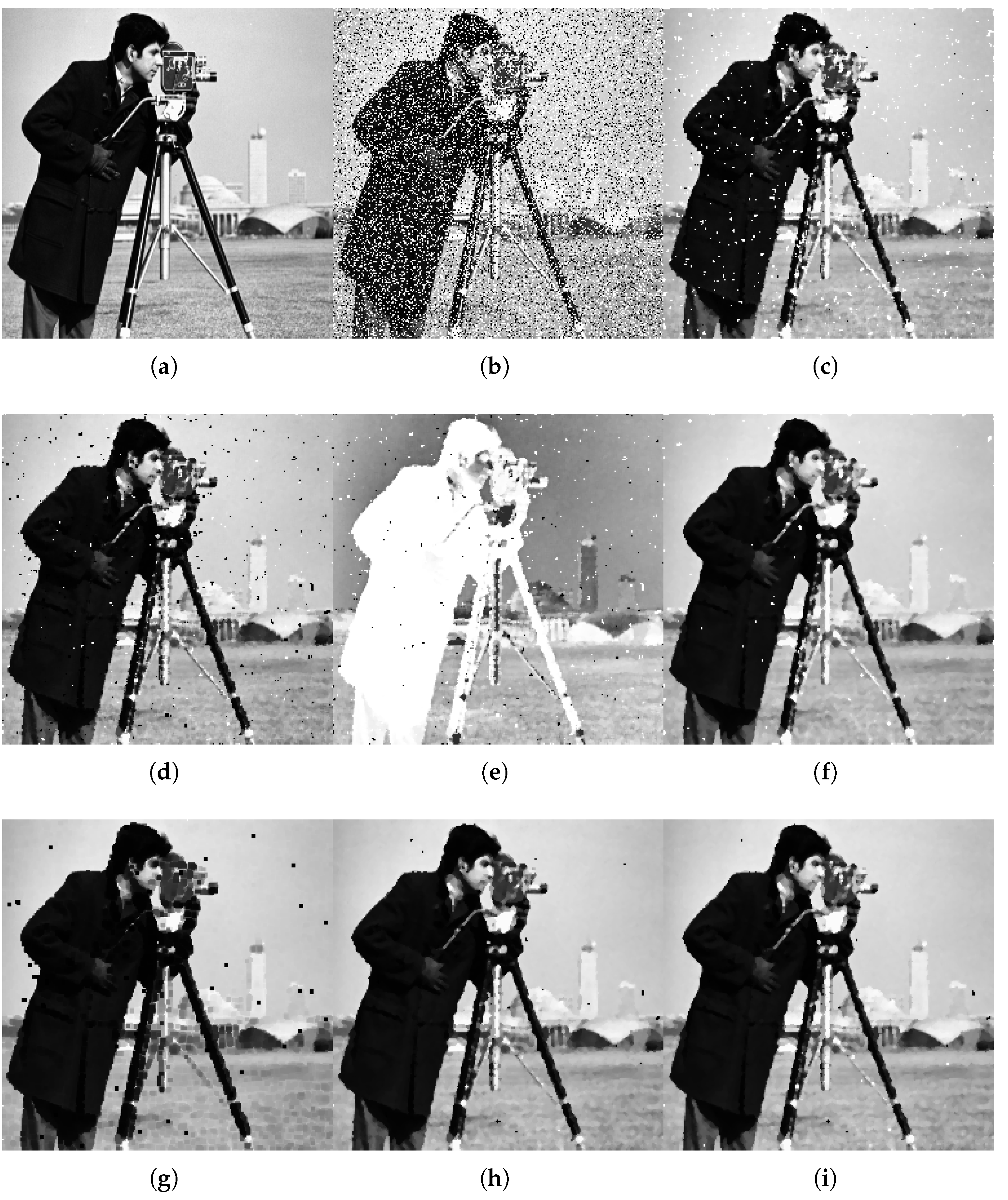
Filtering results of 30% salt-and-pepper noise (2:1 ratio) for different filters are displayed in Figure 6. In our demonstration, we also consider the application of two filters in succession to show the effect of the composition of LIT-filters determined by the multiplication and residuum. In Figure 6c–e, one can see the results of the median filter and the LIT-filter with the multiplication (M-LIT-filter) with the fuzzy measure $\mu ={\mu }_{0.56,0.67}^5$, and the reverse LIT-filter with the multiplication (M-reverse LIT-filter) with the complementary fuzzy measure $\nu$ derived from $\mu$. By adjusting the fuzzy measure $\mu$, we can remove more salt noise, see Figure 6d, compared to the median filter, see Figure 6c, with the presence of a higher proportion of pepper noise. The negative image as the result of the M-reverse LIT-filter seems unnecessary at first glance, especially if we want to work with it immediately without further processing. In Figure 6f–i, one can see the results of combinations of two filters. Particularly, we use the double application of the median filter (D-Median filter) and the application of the median filter and then the minimum filter (Min-Median filter). Further, the composition of the LIT-filters with the multiplication and residuum (MR-LIT-filter), where the R-LIT-filter with the N-conjugate fuzzy measure ${\mu }_N^c$ derived from $\mu ={\mu }_{0.5,0.5}^1$ (the same fuzzy measure as for the median filter, see Table 1) is applied on the result of the M-LIT-filter displayed in Figure 6d. Finally, the composition of the reverse LIT-filters with the multiplication and residuum (MR-reverse LIT-filter), where the R-reverse LIT-filter with the N-conjugate complementary fuzzy measure ${\nu }_N^c$ derived from $\mu ={\mu }_{0.39,0.56}^5$ is applied on the result of the M-reverse LIT-filter displayed in Figure 6e. Comparing the results visually, the MR-reverse LIT-filter in Figure 6i provides the best filtering. This claim is also underlined by the highest PSNR among others in

Table 2. PSNR for different methods of filtering of salt-and-pepper noise.

Filters	PSNR for 30% Noise (dB)	PSNR for 40% Noise (dB)
Median filter	18.416	13.552
M-LIT filter	18.933	16.675
D-Median filter	20.614	15.714
Min-Med filter	16.496	17.192
MR-LIT-filter	21.372	18.939
MR-reverse LIT filter	21.373	19.789

.

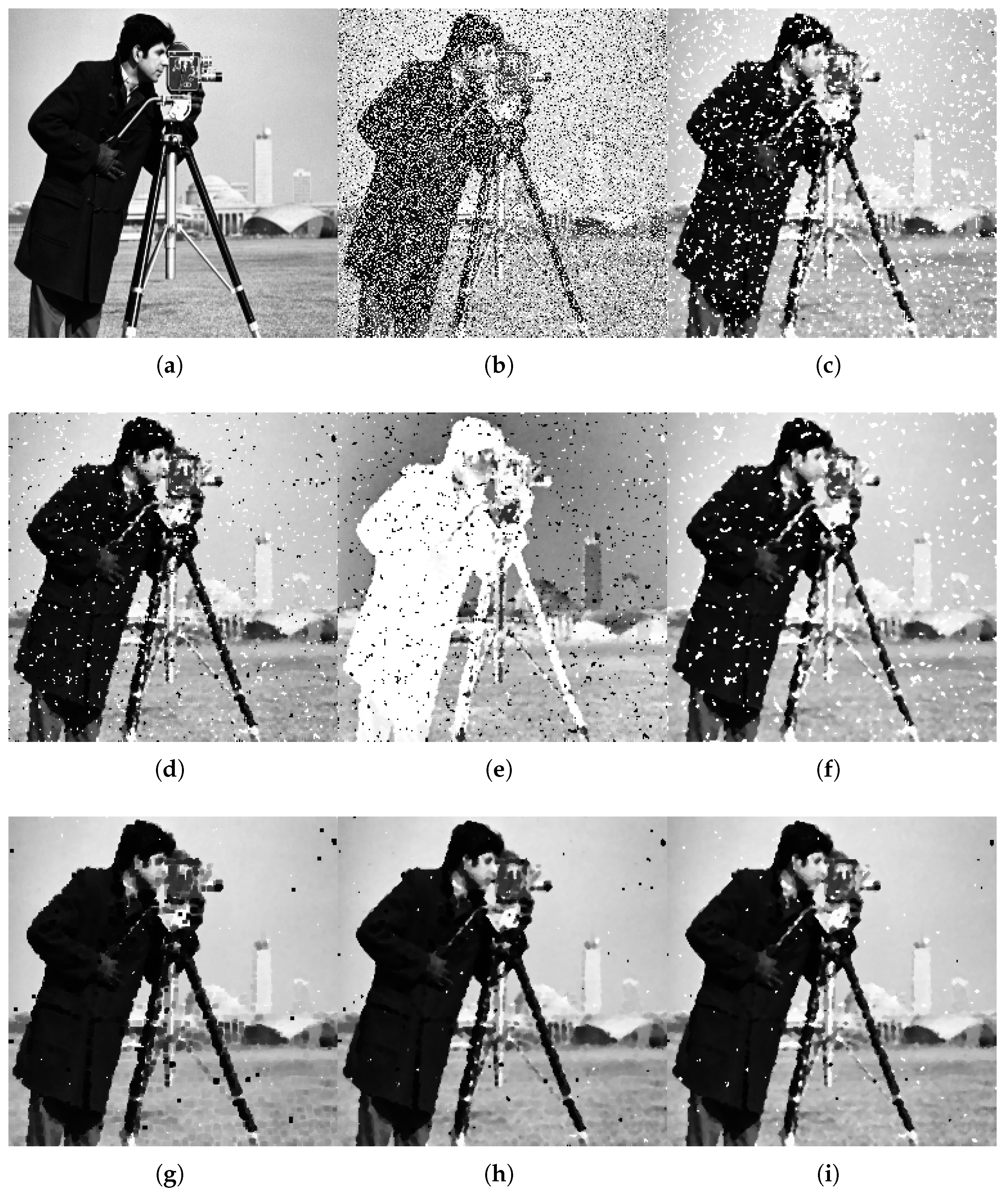
Filtering results of 40% salt-and-pepper noise (3:1 ratio) for different filters are displayed in Figure 7. We consider the same filters as in the previous case. The M-LIT filter has the same fuzzy measure as above. For the MR-LIT-filter, we consider the conjugate fuzzy measure ${\mu }_N^c$ derived from $\mu ={\mu }_{0.23,0.5}$ in the setting of R-LIT-filter, which is applied on the result of the M-LIT-filter in Figure 7d. The M-reverse LIT-filter and MR-reverse LIT-filter have the same setting as in the previous case. Again, the MR-reverse LIT-filter provides the best result both visually and supported by the highest PSNR (see Table 2).

To summarize the results, the filters based on (reverse) integral transforms seem to be useful in filtering non-uniform salt-and-pepper noise from images. For the sake of comparison, the only parameter here was the fuzzy measure whose setting improves the results for the median filter. The further development of more sophisticated filters based on (reverse) lattice integral transforms is the subject of future research.

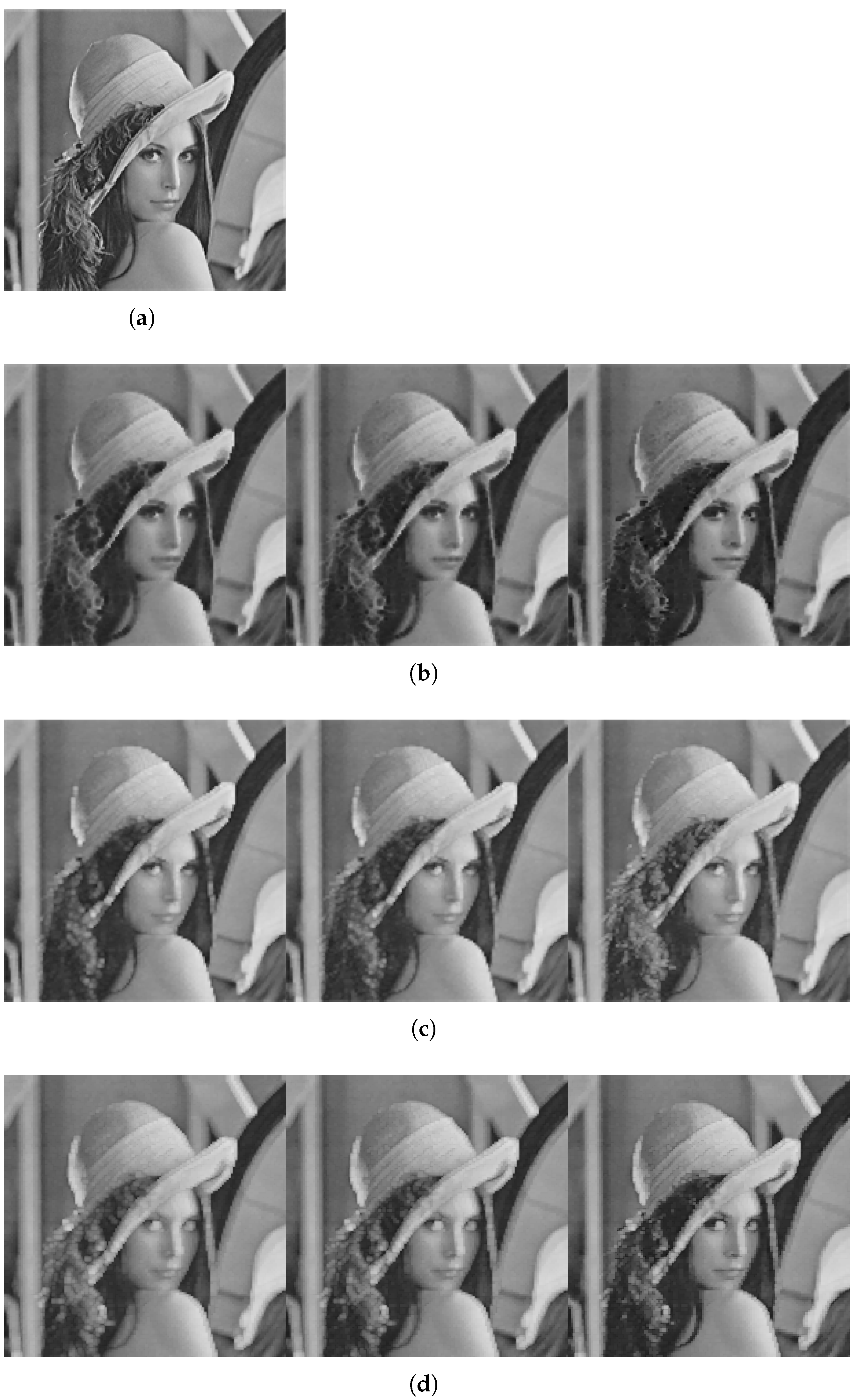
4.2.2. Image Compression and Decompression

For illustration, we use the Lena image (256 × 256) and the compression ratio of 4:1, that is, the shift is $\varrho =2$. We consider the window of size 5 × 5 with the weights equal to 1 around the center and other less than 1, more specifically, $w_{ij}=1$ for $i,j\in [-3,3]$ and $w_{ij}<1$, otherwise. The respective integral kernel is denoted by K. Additionally, we consider $\lambda \in \{0.5,1,2\}$, which specifies the operations used.

For LIT-compression, we consider the fuzzy measure $\mu ={\mu }_{0.16,0.36}^5$, and the remaining fuzzy measures are derived from $\mu$ as follows: ${\mu }_N^c$ is the conjugate fuzzy measure to $\mu$, $\nu ={\mu }^N$ is the complementary fuzzy measure, and ${\nu }_N^c$ is the conjugate complementary fuzzy measure to $\nu$. The results of LIT-compression of the Lena image for different settings are displayed in Figure 8 (the figure is partially adopted from [8]). In particular, the multiplication-based (M-) LIT-compression and residuum-based (R) LIT-compression are presented in Figure 8a,b. The negative output image for the multiplication-based (M-)reverse LIT-compression and the residuum-based (R-)reverse LIT-compression can be seen in Figure 8c,d.

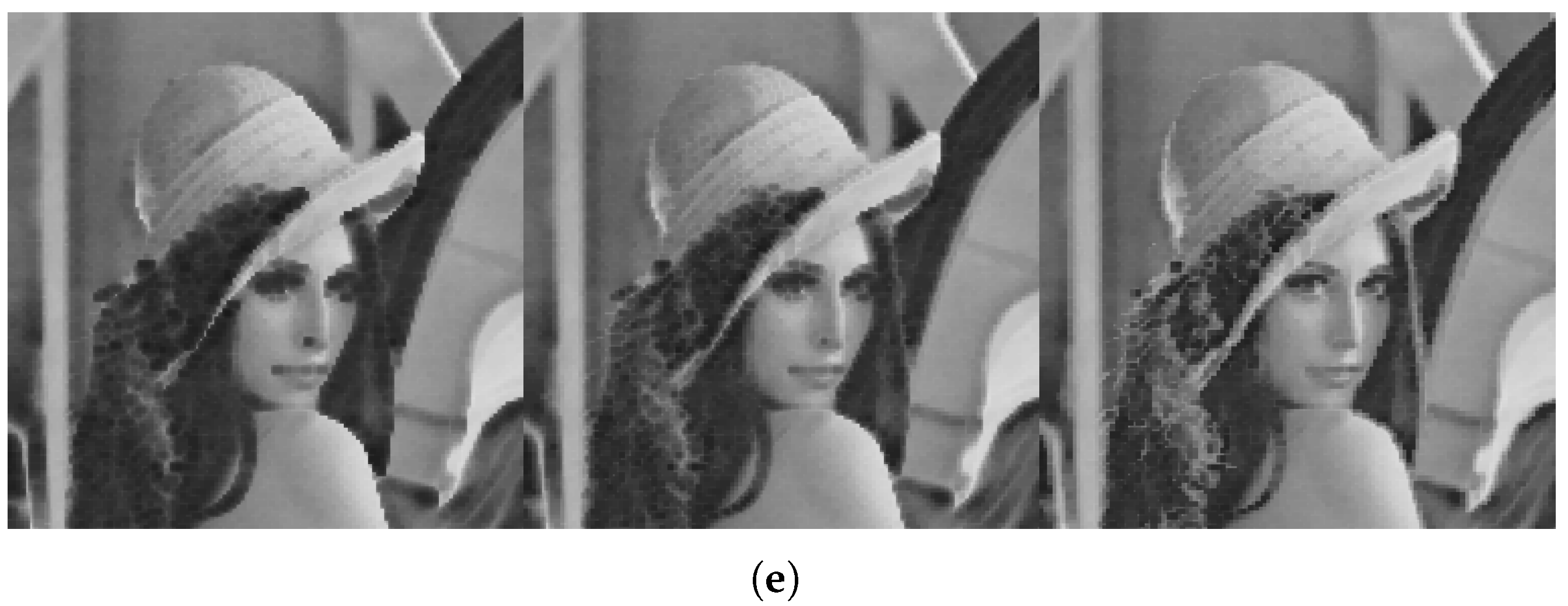
For LIT-decompression, we consider the highest fuzzy measure as ${\mu }^{\prime }$ on $\mathcal{P}(D_{\varrho ,u,v})$ and the remaining fuzzy measures are again derived from ${\mu }^{\prime }$ as for $\mu$, where we use ${\nu }^{\prime }={\mu }^{\prime N}$. The reason for setting ${\mu }^{\prime }$ is the fact that the cores of the inverse integral kernel $K^{-1}$ have the form of singleton, two, and four element sets. Therefore, according to Theorem 4 and the fact that we consider a symmetric fuzzy measure (see Remark 1), we must assign the fuzzy measure ${\mu }^{\prime }$ equal to 1 to all singletons leading to the highest fuzzy measure. The results of the decompression of the compressed Lena image in Figure 8 for different settings are shown in Figure 9 (the figure is partially adopted from [8]). The (reverse) LIT-image decompression always uses the adjoined operation to that which is applied in the LIT-image compression; i.e., the R-(reverse) LIT-decompression is applied to the M-(reverse) LIT-compression, where the residuum (R) is an adjoined operation to the multiplication (M), and vice versa.

In principle, lattice integral transforms lead to lossy (irreversible) compression, and the question is whether the quality of reconstructed images can be improved by appropriate parameter settings, which is the subject of our future research. To compare the quality of Lena image decompression for the various types of LIT-decompression, we calculated the PSNR for each reconstructed Lena image. The results are shown in

Table 3. PSNR for various types of decompression of the 4:1 compressed Lena image by LIT-compression.

$\mathit{\lambda }$	Type of Decompression
	R-LIT	M-LIT	R-Reverse LIT	M-Reverse LIT
0.5	22.2247	21.6284	21.0906	19.8279
1	22.0335	21.4833	20.6404	20.7553
2	19.2163	18.0559	16.4282	18.986

, according to which the best decompression is obtained by the R-LIT-decompression with $\lambda =0.5$ (the left image in Figure 9b).

4.2.3. Opening and Closing

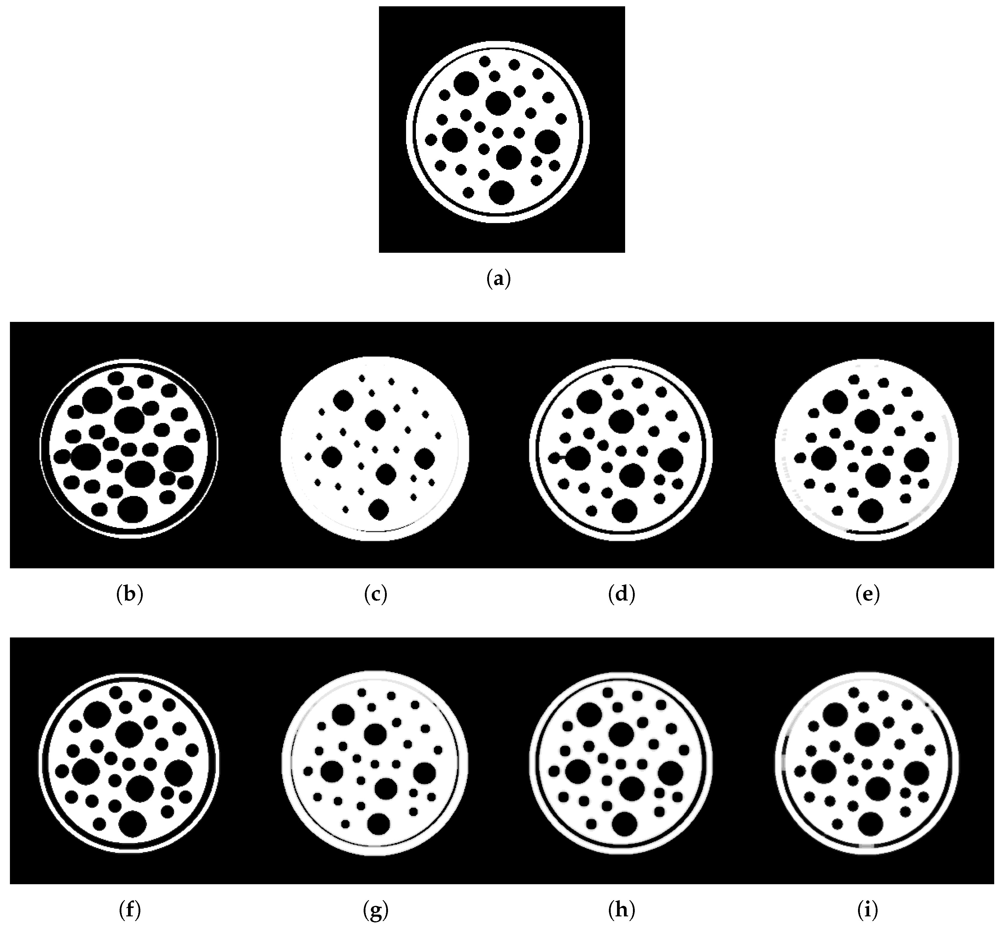
For the last illustration in this paper, we use a 300 × 300 binary image with black balls inside a white circle, which can be seen in Figure 10a. Similarly to compression, we consider the window (structuring element) W of size 5 × 5 with the weights equal to 1 around the center and other less than 1.

By setting the window W, the effect of the morphological operations can be seen on white pixels. As we stated above, in our case, opening and closing operations are fuzzy morphological operations that can be expressed in terms of lattice integral transforms as compositions of fuzzy morphological erosion and dilation.

The results of fuzzy morphological erosion, dilation, opening, and closing for the considered image with respect to the given window are shown in Figure 10b–e. For example, we can see that the white space erodes in Figure 10b and is extended in Figure 10c. For comparison, we consider the LIT-dilation defined as the $(K_W,\mu ,\otimes )$-lattice integral transform with $\mu ={\mu }_{0.12,0.24}$, which is close to the highest fuzzy measure ${\mu }^{\top }$, and the LIT-erosion as the $(K_W,{\mu }^{\prime },\to )$-lattice integral transform with ${\mu }^{\prime }={\mu }^c$, which is close to ${\mu }^{\perp }$. Further, we use the t-norm $T_{\lambda }^{SS}$ and its residuum ${\to }_{T_{\lambda }^{SS}}$ with $\lambda =1$ in the definitions of lattice integral transforms. The LIT-opening is defined as the composition of LIT-erosion and LIT-dilation, and vice verse for the LIT-closing. The results of all modified fuzzy morphological operations are displayed in Figure 10f–i. The effect of the newly defined conjugate fuzzy measure ${\mu }^{\prime }$ in the LIT-erosion is obvious and consists in a smaller erosion of white part in the image in contrast to the fuzzy erosion. The opposite effect can be recognized for the LIT-dilation defined by the fuzzy measure $\mu$. The LIT-opening provides a better restoration of the original image than fuzzy opening, and the LIT-closing leaves more of the black circle than the fuzzy closing. Interestingly, morphological operations based on lattice integral transforms better preserves the shape of black balls in image.

4.3. Remark on Method Complexity

The complexity of the method depends on the implemented algorithm. In case the output pixel of the median filter is calculated by the brute-force method, i.e., first a list of pixel values in the filter window (kernel) is built, then it is sorted and finally the median is determined as the middle value in the list, the complexity of the algorithm is $\mathcal{O}(R^{2}logR)$ for a window of size $R\times R$ (see, e.g., [34,35]). When a constant number of possible pixel values is considered, as in the case of 8-bit images, a bucket sort can be used resulting in $\mathcal{O}(R^2)$ complexity [34]. Fast algorithms for median filters use a histogram instead of a sorting algorithm to calculate the median with $\mathcal{O}(1)$ complexity. The classical algorithm proposed by Huang et al. in [36] and used in virtually all publicly available implementations, provides $\mathcal{O}(R)$ complexity (see, also, [34]). An improvement of the Huang’s algorithm was proposed in [34] which decreases the complexity of the median filter to $\mathcal{O}(1)$. Nevertheless, as was noted in [35], a disadvantage of this method is a high memory consumption and a complicated implementation in hardware. In [37], the authors show that even for the weighted median filter the standard complexity $\mathcal{O}(R^2)$ can be reduced to $\mathcal{O}(R)$ with the help of a joint histogram. This is possible under the assumption that the weights do not varies according to feature distance. It should be noted that all approaches reducing the complexity of the (weighted) median filter to $\mathcal{O}(R)$ or even $\mathcal{O}(1)$ use a trick that simplifies the histogram update, since this step is crucial to determine the complexity of the algorithm.

To discuss the complexity of a non-linear filter based on lattice integral transforms, we present the basic steps of the method in Algorithm 1, where the operation ⋆ represents one of the operations ⊗ and →.

Algorithm 1 Non -linear filter based on lattice integral transform.

Input: Image I of size $N\times M$, window $W=\left\{w_{k,\ell }\right\}$ of size $R\times R$ with $R=2r+1$ Output: Image J of the same size as I  Initialize pixel neighborhood $H=\left\{H_{k\ell }\right\}$  for $i=1$ to N do   for $j=1$ to M do    for $k=-r$ to r do     for $\ell =-r$ to r do      Calculate pixel neighborhood $H=\left\{H_{k\ell }\right\}$ with $H_{k\ell }=I(i+k,j+\ell )\star w_{k,\ell }$     end for    end for    $J(i,j)\leftarrow \mathrm{Integrate}(H)$   end for  end for

The algorithm shows that the list H representing the “weighted pixels” in the neighborhood must be updated at each step, resulting in $\mathcal{O}(R^2)$ complexity. To calculate the Sugeno-like integral of the list H, we need three consecutive procedures (cf. Corollary 1): sort the list H, multiply it by the list of measure values, and find the maximum, which results in $\mathcal{O}(R^{2}logR)$ complexity, i.e., the complexity of sorting the list H, which is the most complex procedure of all. If a constant number of possible pixel values is considered, the complexity can be reduced to $O(R^2)$ by using the bucket sort. To summarize, the complexity of the proposed filter is the same as the complexity of the weighted median filter. Since the scheme of the compression/decompression algorithm is analogous to Algorithm 1, only the image size J in the output is different, the same complexity also holds for these tasks.

5. Conclusions

In this paper, we demonstrated an application of (reverse) integral transforms for lattice-valued functions to image processing. We introduced two types of lattice integral transforms and showed some of their properties, including the preservation (reversion) of constant functions, which is an important property considered in image processing. Specifically, we used lattice integral transforms for image filtering, compression/decompression, and extension of fuzzy morphological opening and closing operations. The proposed methods are illustrated on different images. The advantage of the application of lattice integral transforms in image processing is a wide range of settings where the user can combine the integral kernel (window), fuzzy measure, and the definitions of multiplication, residuum, and negation operations. The provided demonstration cannot be taken as a comprehensive presentation of image processing methods based on lattice integral transforms, but rather as a new and perspective approach that could expand the class of similar methods as non-linear filters or (fuzzy) morphological operations.

In future research, we plan to analyze in detail the relationship between the setting of lattice integral transform parameters and the results for various tasks in image processing and compare outputs also with other non-linear approaches on a large image datasets. In addition, we also intend to apply the proposed approach to color images or videos as follows. The movie is decoded into individual frame(s) and accessed separately. The color image is then divided into color channels and independently processed one by one. The standard RGB color model is suitable for noise filtering. For compression, it is preferable to use the YUV color model, where U and V are compressed more strongly than the Y component that contains information important to human perception. Finally, the proposed method can be used as a pooling layer in deep neural networks. Here, pooling is a layer without trainable parameters that reduces spatial dimension, and it is one of the basic layers used in convolutional neural networks. Contrary to standard pooling operations of mean or maximum, we access the spatial information in a more sophisticated way, from which a neural network should benefit. The implementation and confirmation of this hypothesis is our next challenge.