Application of Graph Structures in Computer Vision Tasks

Abstract

On the one hand, the solution of computer vision tasks is associated with the development of various kinds of images or random fields mathematical models, i.e., algorithms, that are called traditional image processing. On the other hand, nowadays, deep learning methods play an important role in image recognition tasks. Such methods are based on convolutional neural networks that perform many matrix multiplication operations with model parameters and local convolutions and pooling operations. However, the modern artificial neural network architectures, such as transformers, came to the field of machine vision from natural language processing. Image transformers operate with embeddings, in the form of mosaic blocks of picture and the links between them. However, the use of graph methods in the design of neural networks can also increase efficiency. In this case, the search for hyperparameters will also include an architectural solution, such as the number of hidden layers and the number of neurons for each layer. The article proposes to use graph structures to develop simple recognition networks on different datasets, including small unbalanced X-ray image datasets, widely known the CIFAR-10 dataset and the Kaggle competition Dogs vs Cats dataset. Graph methods are compared with various known architectures and with networks trained from scratch. In addition, an algorithm for representing an image in the form of graph lattice segments is implemented, for which an appropriate description is created, based on graph data structures. This description provides quite good accuracy and performance of recognition. The effectiveness of this approach based, on the descriptors of the resulting segments, is shown, as well as the graph methods for the architecture search.

1. Introduction

Recently, the computer vision applications have become more and more relevant. Among these key computer vision system tasks, are the actual image recognition, object detection and image segmentation. Image processing algorithms are required in various fields of science and technology: from access control systems to intelligent systems for detecting defects in reinforced concrete products. In recent years, various methods, based on deep neural networks, have become popular in this area. The hidden task of any computer vision neural network is to form the features that describe objects in the image and classify them correctly.

However, this approach has a number of disadvantages. The first weakness for neural networks is the computing power. The training process to acquire sufficiently efficient neural networks, in terms of recognition accuracy, requires a lot of processors and a long training time. Moreover, the vast majority of deep learning models needs millions of well-labeled examples for training purposes. Usually, in a number of applied tasks, it is impossible to provide sufficiently large training samples in advance. In this case, it is possible to use the classical mathematical methods of image processing. Unfortunately, it has been shown that they are inferior to neural network models for large image datasets.

A reasonable alternative approach to improve the performance of mathematical methods, is to obtain descriptive feature sets by analogy with neural network models. The description of the structure and the connections between pixels, provide useful information for extraction and can be represented as a graph with their respective connections. Such an approach will potentially improve the image processing quality, compared to the classical mathematical methods. Furthermore, in conditions of insufficient data, graph methods for image recognition can be more efficient than deep neural networks, because the latter are underfitted. Next, let us consider both neural network approaches to solving the computer vision tasks and graph methods for image processing.

The novelty of this article is in the use of graph-based segmentation results for the collection of the descriptors for different objects presented in the image datasets. So, the suggested approach extends the graph segmentation method to recognition. Once the model training is completed, it is possible to use the descriptors for recognition, which make processing faster than using transformers and some convolutional networks. Furthermore, the new approach for searching optimal architectures, is suggested in the text. It provides efficiency (in terms of accuracy) and gains, but requires a lot of computational power for training.

2. Related Works

One of the most popular computer vision tasks is object recognition. Modern applied solutions are intelligent systems, which often work quickly and efficiently in conditions of sufficient data, during training. However, the network architecture design is particularly important when there is insufficient training data. At the same time, classically, the development of image processing systems began with the use of random processes and mathematical field models [1,2,3,4]. Such an approach provides the replicated data for vision systems. So, mathematical models are still used in a number of tasks nowadays, especially in image preprocessing.

In addition to replicating images using statistical generative models, the second way to deal with the lack of data is by augmentation. For such a data type as an image, there are effective augmentation algorithms [5,6].

However, if augmentations do not improve the training results, the next suitable solution is to collect additional images or move on to search for another neural network architecture. At the same time, the design of such architectures is often performed by the researcher, based on their own experience. There is currently no unified approach to choosing the neural network architecture. Widely known methods are methods using the special descriptors of important objects in images [7]. In particular, the authors of [7] showed a gain in the recognition efficiency of objects that do not have pronounced textures, using a simple support vector machine, compared to the deep learning technologies [8]. However, machine learning methods are not always superior to deep learning methods. Therefore, the transfer of learning technologies has also been widely used [9,10,11].

Such training occurs by adjusting the last or the last few layers of the model to the data of a particular recognition task. The first high-performance results were obtained using the convolutional neural network AlexNet [12], named after the main developer Alex Krizhevsky. An important algorithm for optimizing training processes, which reduces overfitting, is Drop Out [13]. The method allows to reset the weight coefficients, which can be considered analogous to removing links in a graph structure. Thus, the networks become less prone to overfitting. Further development consists in the complication of architectures, the increase in layers, neurons, the connections between and within, which can also be described by the graph structures. However, the principle of action with convolution remains. Examples of such networks are Inception [14], Xception [15], ResNet [16] and VGG [17]. For example, in [17], the authors used a deep architecture with 19 layers of convolution and pooling. In this model, a sufficiently small size (3 × 3) was chosen for the convolution kernel. The network [14] was already saturated with 22 layers, although the architecture of the neurons’ arrangement in width and depth allowed the Inception network [14], in 2014, to be the most efficient network in the ImageNet image recognition competition. Then, there was an increase in the number of parameters and layers. This is the most generalized trend in deep learning so far.

A closely related problem with image recognition is object detection [18], when an object occupies only a region of the whole area of the image. In fact, the question arose about how to select these regions, so the changes that needed to be made to the architecture of the convolutional networks, were changes related to the proposal of the regions, upon which the recognition problem can be solved. This approach gives rise to a line of two-pass detection algorithms, and in particular, R-CNN models [19]. The models with the Fast R-CNN architecture [20] and the Faster R-CNN models [21], that optimize the detection solution, are emerging. The development of such solutions became possible due to the fundamental expansion of the architecture, but without the emergence of fundamentally new ideas for organizing the connection of weights within and between layers. Then, there are convolutional networks that can work even faster, because detection and localization are performed in one pass. These are called single-pass detectors and include the You Only Look Once (YOLO) model, used in the object detection in images and videos [22]. Solutions for another problem, such as segmentation or instance segmentation, were obtained by modifying the R-CNN architecture. One of the popular models today is Mask R-CNN [23].

However, an interesting development in the field of network architectures has been the adoption of transformers from natural language processing (NLP) [24,25,26]. Since in NLP, such architectures operate with embeddings (parts of text), in vision, they operate with local areas, but take into account the spatial structure. In [27], the authors proposed a multi-scale deformable transformer-based network for the classification of glands, into normal and intestinal metaplasia gastric glands. In [28], the authors wrote about using transformer models for face recognition. Unfortunately, the main disadvantage of such solutions is their complexity and low performance.

Finally, there are also graph solutions in computer vision [29,30,31], which are considered in more detail. In [29], the authors wrote of the methods for processing images in industry with a different geometry. The graphs are mostly used for taking into account some deformations. Recent studies introduced combined graphs and convolutional methods for image classification [30], based on embedding. However it shows poor results in some datasets. Significant results were obtained with combined graph methods for satellite images [31], however such algorithms required a lot of data with a high resolution.

The most common shortcoming of the widely used convolutional neural network models, is their weak invariance, i.e., different rotations, scales, and lighting angles on test images that can lead to errors in recognition if the training sample is not saturated with such examples [32]. Actually, the problem of weak invariance is a common problem for small datasets that sometimes can be solved by using advanced augmentation [33]. The second disadvantage is the loss of connection between the different parts of the object, when applying convolutions. In [34], it is shown how the final output of a convolutional network can be affected by changing just the brightness value of one pixel. In [35], it is noted that the convolutional network evaluates the image by the totality and the presence of the features, but does not take into account the relationship between them. 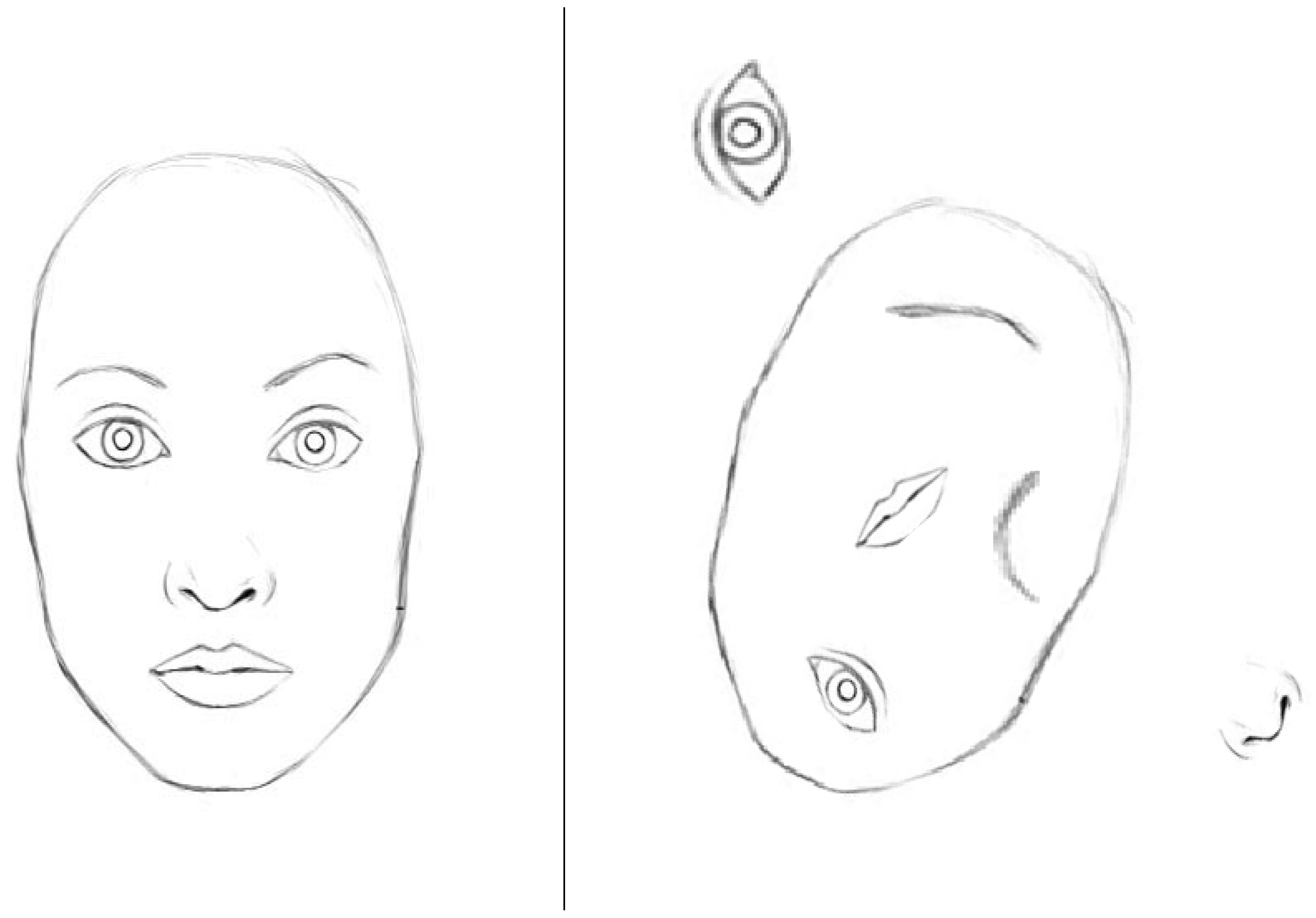Figure 1 shows an example of two images that will be recognized by the convolutional network as a face. The first is a real face, but the second is only a set of facial features. The solution of the spatial dependency problem is represented in [36]. However, such a neural network has a more complex architecture, namely it has a number of recurrent layers that require more memory and computing power. Finally, the main disadvantage of convolutional neural networks, is their need for retraining, when adding a new class.

Figure 1. Example of an inaccurate classification, in the presence of sufficient separate features.

With the advent of the Leonhard processor, ideas about building neural networks on graphs arose. This can provide a better performance and power efficiency. The idea is that initially there are no semantic structures, a predetermined architecture, and the graph of the neural network is built in the course of the training and understanding the validation data. Leonhard (named after Leonhard Euler) is a fundamentally new processor for processing sets, data structures and graphs [37]. This processor executes a set of instructions from discrete mathematics and works not with numbers, but with sets. This is the so-called DISC command set (discrete mathematics instruction set computer). Thanks to this approach, Leonhard also works effectively with graph structures. The developers note that the Leonhard microprocessor takes 400 times fewer crystal resources than a single core of the Intel Core family, and also consumes 15 times less energy than a single core of the Intel Core family.

The general statements [38] that must be observed when organizing a graph recognizer are as follows:

(1)

It is necessary to set rules where the components of the object are compared to the components of the graph.

(2)

Determine the type of these correspondences. They can be unidirectional, bidirectional or multi-valued.

(3)

Determine the way to display the properties and components of the object in the characteristics of the graph.

Next, the article considers the datasets that are used for the experiments and the preprocessing methods. Then, the text deals with two novel approaches. The first obtains and evaluates the object descriptors, using the ART transformation. The main idea of the second is to model the adaptive architectures with the graph connections in a neural network, in width and depth. The transformation of the initial data, the images themselves, into graph structures, and the search for architectures in the form of connected graphs from neurons, are also presented.

3. Materials

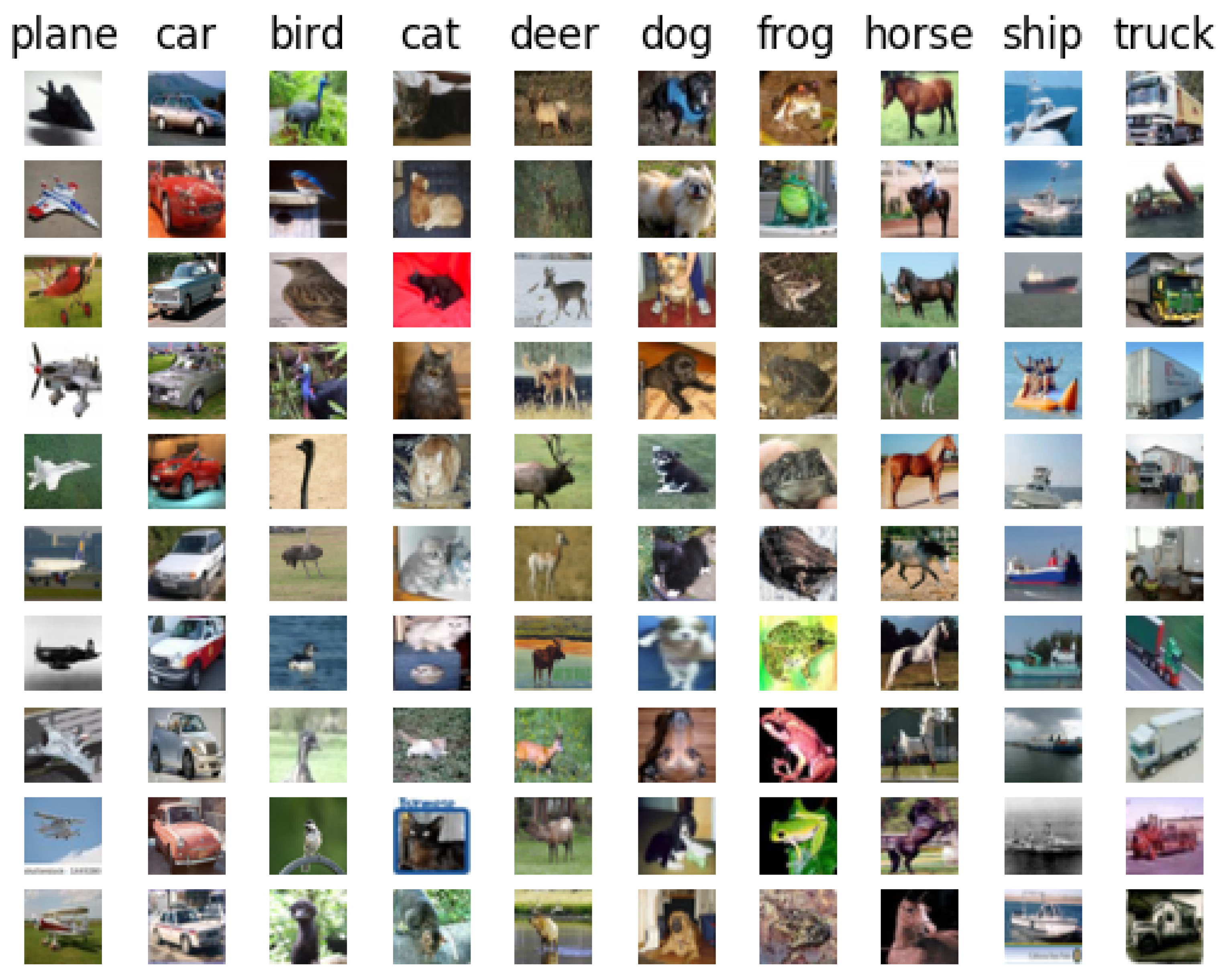
First, it is necessary to consider the datasets that will be used in the experiments. The first dataset is CIFAR-10. The dataset includes 60,000 RGB images. The sizes are 32 × 32 pixels. All images are classified into 10 classes and the data is absolutely balanced. The training set consists of 50,000 images, and the remaining 10,000 images are used for the test. The presented classes are: frog, truck, deer, automobile, bird, horse, ship, cat, dog and airplane. Figure 2 shows some example images from CIFAR-10.

Figure 2. CIFAR-10 images.

So, from Figure 2, it can be seen that all images are standard in this dataset. Preprocessing is needed for the normalization of the data. Prior to the training, the normalization layer provides zero mathematical expectations and unit standard deviations.

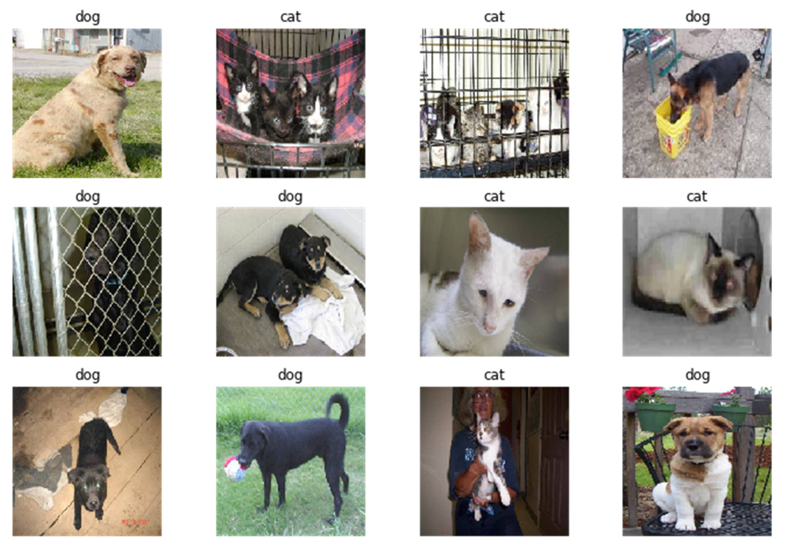
Our second dataset is the Kaggle competition dataset called Dogs vs Cats. It consists of different sized images. As for the classes, it has 25,000 balanced images of dogs and cats for the training and the test. The sample split will be performed with 25% for the test images. The sizes of the images are different, so it is necessary to create standard sized images for the transfer learning and projected architectures. The scaling method is also used. All brightness values are divided by 255, so the possible values are from 0 to 1.

Figure 3 shows some examples from this dataset.

Figure 3. Dogs vs Cats images.

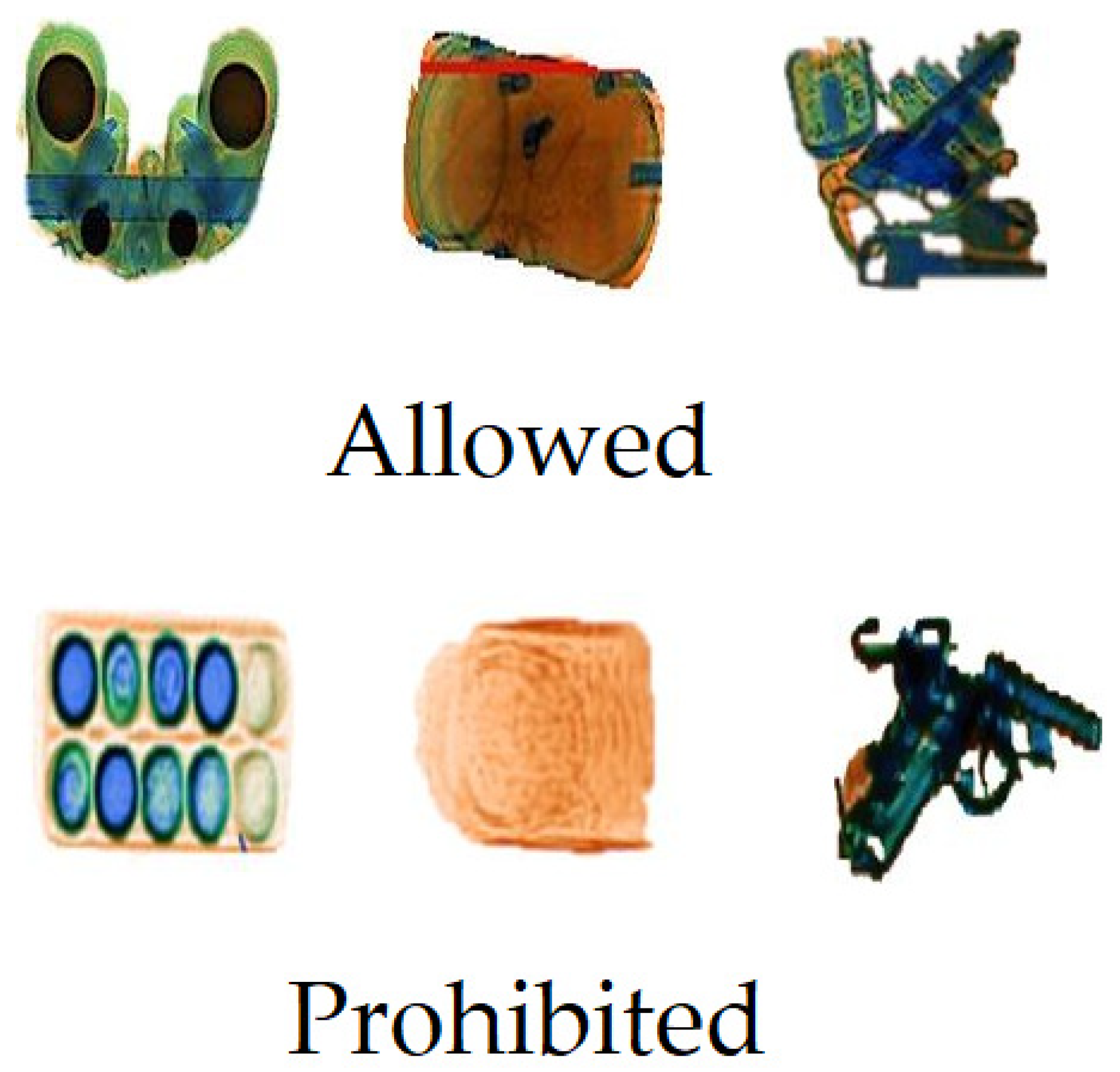
Finally, the experiments also use a X-ray image dataset of baggage and cabin luggage. It is unbalanced data, which consists of 200 images of prohibited items and 280 images of allowed items. The sizes are standard and they are 125 × 125 pixels. For preprocessing, gray scaling and normalization are used. Figure 4 shows some examples from the X-ray image dataset.

Figure 4. X-ray images.

It should be noted that the processing of such images is different from the processing of standard optical images. The results for the graph method will also be interesting. Preprocessing for the graph method uses a Gaussian filter with $\sigma =0.8$ to blur the edges of the objects in the images, for a better segmentation.

4. Methods

Let us transform a two-dimensional image into a graph representation. To do this, it is logical to use a lattice or grid structure. Let us also represent each pixel of the image as a vertex, in which the brightness value of the pixel is written. Each pixel has connections with the pixels located on its left, right, top and bottom. The edges can be weighted and the information concerning the difference in brightness can be stored. Such edges may allow the selection of optimal routes for efficient processing. Often there is no sharp change in the brightness inside of the objects.

In [39], an efficient solution for the segmentation on the graphs, based on the Kruskal algorithm, was proposed. The solution can be improved by applying Gaussian filters [40] for a smoother localization of the different image segments.

Based on the Kruskal algorithm, a spanning tree is built. Let pixels be vertices $x(i)$, then the edges symbolized connections can be described as $r(x_i,x_j)$. Such an edge, characterizes the connection between $i$-th and $j$-th pixel. Such edges will be characterized by links or weights $w(r(x_i,x_j))$. The task is to find the minimum remaining tree in such a graph, for which the total weight of all edges will be minimal, and not a single pixel will be discarded.

Next steps operates the principle of the algorithmic clustering. For each vertex, a set is created and these vertices are further combined into segments. At the same time, it is clear that the vertices in such a segment form the minimum remaining tree. The Gaussian filter can be applied for the image preprocessing with different variances, as it will smooth out the input image, even slightly blurring it.

To calculate the weight of the edges, it is possible to use numerical RGB values, i.e., the vector distance in a 3D space. To improve the quality, other color spaces more characteristic of the human visual system, can be used. Figure 5 shows the source image and an example of the segmentation results.

Figure 5. Segmentation, based on graphs [39].

Following the division into segments, it is necessary to determine what can be written into the descriptors. Such descriptors should store information about each segment, as accurately as possible. Then, it is necessary to search for similar segments, to collect the personal knowledge base. Let us divide the descriptors into two classes: the shape description and the color description. When describing a color, the gradient should also be taken into account. It is clear that the shape is insufficient for the accurate classification, due to the fact that objects are represented by projections, can be overlapped by other objects, etc. It is also not enough to use the color information alone, in the vast majority of tasks.

The zone shape descriptor includes elements of the so-called angular radial transform (ART). Let us write such a transformation, as an expression:

$$F_{nm}=⟨V_{nm}(\rho ,\theta ),f(\rho ,\theta )⟩={\displaystyle \underset{0}{\overset{2\pi }{\int }}{\displaystyle \underset{0}{\overset{1}{\int }}{V}_{nm}^{*}(\rho ,\theta ),f(\rho ,\theta )}\rho d\rho d\theta }$$

(1)

where $F_{nm}$ is the ART conversion factor of the order n and m, $f(\rho ,\theta )$ is the description of the image brightness distribution in the polar coordinate system, $V_{nm}(\rho ,\theta )$ is the basis function of the transformation.

In Expression (1), the basis function can be represented as the expansion of the angular and radial components:

$$V_{nm}(\rho ,\theta )=A_m(\theta )R_n(\rho )$$

(2)

Finally, the following formulas can be used to calculate the components in Expression (2):

$$A_m(\theta )=\frac{1}{2\pi }\exp (jm\theta ),$$

(3)

$$R_n(\rho )=\{\begin{array}{c}1,\begin{array}{cc}if& n=0\end{array},\\ 2\cos (\pi n\rho ),else.\end{array}$$

(4)

Thus, Expressions (1)–(4) describe a method for obtaining the zone type descriptors. Such descriptors represent the shape of the objects for future recognition.

Obtaining a segment descriptor (ArtDE) involves the following steps:

(1)

Generation of the basis function. Since the basis function is separable, then $V_{nm}(x,y)$ is calculated immediately in Cartesian coordinates, so as not to translate from polar coordinates $V_{nm}(\rho ,\theta )$ to the Cartesian coordinates at a later stage. To do this, a set of ART basic functions is created in the form of two four-dimensional arrays, for the real and imaginary parts, respectively.

(2)

Size normalization. The center of mass of the object is mapped to the center of the lookup table. If the size of the image and the lookup table are different, then the linear interpolation is applied to map the image to the corresponding lookup table. Here, the object’s size is defined as twice the maximum distance from the object’s centroid.

(3)

ART transformation. The real and imaginary parts of the ART coefficients, ART_R (12) (3) and ART_I (12) (3), respectively, are calculated by summing the result of the multiplication of a segment pixel by the corresponding position in the lookup table in the raster scan order. Twelve angular and three radial basis functions are used here.

(4)

Zone normalization. The value of each ART coefficient (ART(m) (n)) is calculated by taking the square root of the sum of its imaginary and real parts squared. The resulting values are further divided by the first coefficient (ART (0) (0)) for the normalization.

(5)

Quantization of transformation on 16 levels. Values of the ART coefficients, with the exception of ART_M (0) (0), are quantized by 16 levels, according to Table 1.

Table 1. Correspondence of the ART_M ranges and ART_DE levels.

Range	ART_DE
0.000000000 ≤ ART_M < 0.003585473	0000
0.003585473 ≤ ART_M < 0.007418411	0001
0.007418411 ≤ ART_M < 0.011535520	0010
0.011535520 ≤ ART_M < 0.015982337	0011
0.015982337 ≤ ART_M < 0.020816302	0100
0.020816302 ≤ ART_M < 0.026111312	0101
0.026111312 ≤ ART_M < 0.031964674	0110
0.031964674 ≤ ART_M < 0.038508176	0111
0.038508176 ≤ ART_M < 0.045926586	1000
0.045926586 ≤ ART_M < 0.054490513	1001
0.054490513 ≤ ART_M < 0.064619488	1010
0.064619488 ≤ ART_M < 0.077016351	1011
0.077016351 ≤ ART_M < 0.092998687	1100
0.092998687 ≤ ART_M < 0.115524524	1101
0.115524524 ≤ ART_M < 0.154032694	1110
0.154032694 ≤ ART_M	1111

In such a case, the distance between the two segments can be calculated as the sum of all distance modules of the corresponding ART coefficients.

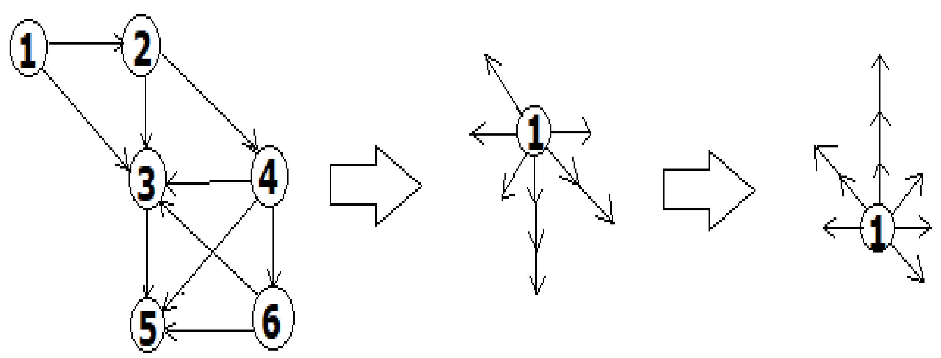
A similar lattice graph is constructed for the gradient, only the output of Kruskal’s algorithm is used. The graph has eight connections and ensures that the descriptor is invariant to the rotations, as shown in Figure 6.

Figure 6. Acquiring a gradient descriptor. Here circles (1–6) are nodes of the image graph.

Similarly, a graph is constructed for the hue descriptor. The general implementation for the efficient graph-based computer vision methods and codes, are provided in GitHub [41]. Our algorithm modified this approach in order to obtain the descriptors using the mathematical calculations represented above.

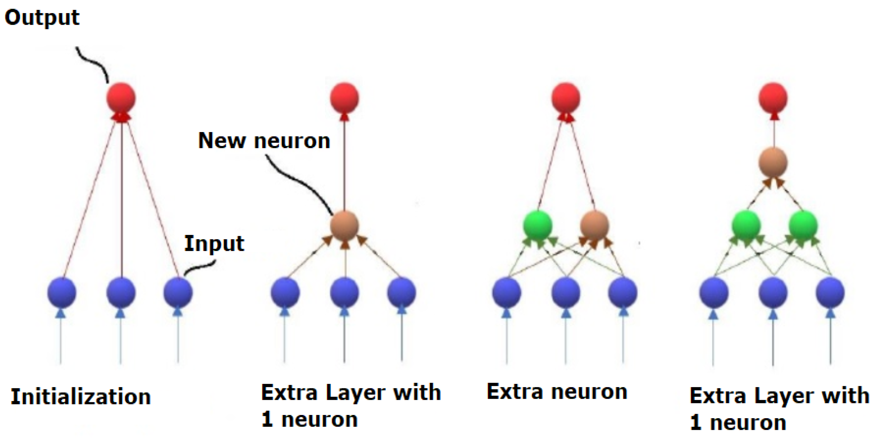
Next, let us consider an example where training is carried out with a conceptual approach. There is no specified network architecture. However, either an increase in the width can occur, i.e., adding new neurons, or an increase in the depth, which means adding new layers. Figure 7 shows the main idea of this approach.

Figure 7. Formation of the neural network architecture in the form of a fully connected multilevel graph.

In this case, the assessment of the need to add a new layer occurs on the basis of the validation set. In the event that the addition of neurons into the current layer does not give an increase, the new layer should be added with one neuron. Then, that algorithm extends this layer by neurons until there is no efficiency increase again. Let us consider the algorithm (Algorithm 1) for the suggested solution, in detail.

Algorithm 1 Optimal architecture search

START Initialize the architecture with one neuron in the hidden layer. Initialize Epsilon for the losses, max depth and max width. Train the architecture using the standard back propagation methods. Evaluate the model in the validation set with the Loss (1,1). Here (1,1) means that the neural network has one neuron in the first layer. Extend the neural network in width by adding one neuron in the current layer. Train the new architecture. Evaluate the model in the validation set with the Loss (1,2). Here (1,2) means that the neural network has two neurons in the first layer. While {LOSS (1,I − 1) – LOSS (1,i) > Epsilon or i < max width}: Repeat the extension in the width, train and evaluate. Extend the neural network in the depth by adding a new layer with one neuron. Repeat steps 3–9 for the Loss (j,i). Stop algorithm when j reaches the max depth and I reaches the max width. END

Thus, for the computer vision tasks, it is possible to reconfigure the last layers of the recognizer in this way.

Next, let us consider the results of such a processing.

5. Results and Discussion

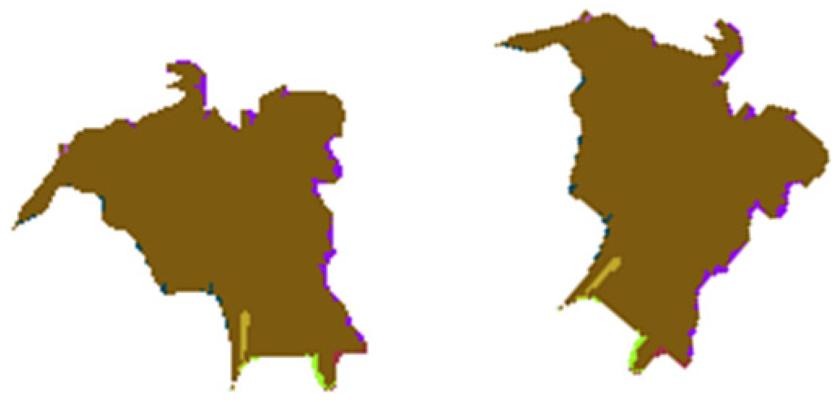
To test the effectiveness of the descriptor invariance, it is necessary to consider the descriptors for images rotated at different angles. Figure 8 shows such images in the example of a recognized palm tree crown, from Figure 5.

Figure 8. Original segment image and rotated 45 degrees.

The ART transformation uses 12 angular basis functions and 3 radial functions. Thus, there are 36 descriptors for the object shape in total. Table 2, Table 3 and Table 4 present the values obtained from the calculation of the first 12 descriptors, the next 12 descriptors, and the last 12 descriptors.

Table 2. Shape descriptors No 1–12.

Location	D1	D2	D3	D4	D5	D6	D7	D8	D9	D10	D11	D12	Delta
Original	13	10	11	4	4	3	15	1	5	13	15	12	17
Rotated	12	8	12	4	5	5	11	2	5	14	13	14

Table 3. Shape descriptors No 13–24.

Location	D1	D2	D3	D4	D5	D6	D7	D8	D9	D10	D11	D12	Delta
Original	15	1	6	11	7	11	7	1	6	15	14	5	18
Rotated	14	3	8	8	6	9	8	2	6	12	13	6

Table 4. Shape descriptors No 25–36.

Location	D1	D2	D3	D4	D5	D6	D7	D8	D9	D10	D11	D12	Delta
Original	10	13	7	16	2	15	13	15	15	16	9	1	27
Rotated	9	10	10	12	4	14	12	12	11	13	10	2

The analysis of Table 2, Table 3 and Table 4 shows that the deviation within one descriptor should not exceed 5 units, and the total is 62. It has been experimentally established that such a difference should not exceed 100 units in total.

Table 5 presents the results of the comparison of the gradient descriptors. All eight pixel links are examined.

Table 5. Gradient descriptor comparison.

Location	Top	Top Right	Right	Bottom Right	Bottom	Bottom Left	Left	Top Left	Delta
Original	1.264	1.042	1.112	0.983	0.876	1.002	1.108	1.203	1.365
Rotated	0.995	0.878	1.064	1.186	1.006	0.855	1.236	0.927

It has been established that the total difference of the normalized descriptors should not exceed two units, and for one direction the allowable deviation is 0.3.

It should be noted that, for the selected pixel in terms of the hue gradient, the full correspondence of the RGB channels was observed.

It also should be noted that all limitations were conducted using, not only one image, but entire datasets, such as CIFAR-10. However, this example shows all transformations for the descriptors more appropriately.

Table 6 shows the results for small dataset of X-ray images. The task is to recognize the prohibited items. It should be noted that there was no augmentation for the source sample. However, test image dataset contains about 20% of rotated images. The modern methods are visual transformers [24] and they are also presented in comparison, as ViT. It is also interesting to evaluate the performance of the models. The processing is performed on Intel Core i7-9700k CPU (Intel Corp., Santa Clara, CA, USA).

Table 6. Graph recognition performance, precision and recall for the X-ray images.

Model	Precision of Prohibited Items	Recall of Prohibited Items	Performance (Frames per Second)
Graph	86.82%	91.32%	21.92
ResNet	88.32%	74.76%	32.55
VGG	89.85%	75.69%	8.65
ViT	86.72%	90.44%	1.28

So, the suggested graph-based approach allows to obtain better results, in the sense of the recall, and it is faster than the VGG model. However ResNet provides better performance characteristics. The problems with the convolutional networks methods are the small training dataset and the unbalanced data (the prohibited samples are fewer than the allowed samples). ViT is very slow. So, the graph solution is seen as optimal here.

Table 7 shows the accuracy results for the Dogs vs Cats dataset. Such metrics are used because of the balanced data.

Table 7. Graph recognition performance, accuracy for the Dogs vs Cats images.

Model	Accuracy	Performance (Frames per Second)
Graph	94.46%	4.89
ResNet	94.81%	8.44
VGG	95.77%	2.73
ViT	96.38%	0.98

The graph method provides average results in general comparison to the other methods. The accuracy is less than the accuracy in the deep learning methods, but the performance is better than with VGG and ViT.

It is obvious that the graph structures make it possible to obtain sufficiently good descriptors of the segments and objects. Moreover, the adaptive design of the architecture of the last layers also allows to optimize the quality of work in the test data.

Table 8 shows the results for the different networks with and without the selection of the output layers on the CIFAR-10 dataset. It is a balanced dataset, therefore, to assess the quality, the metric of the correct recognitions proportion is enough. So the model comparison results are presented with a sense of accuracy.

Table 8. Comparison of the recognition of the accuracy and training time.

Model	Accuracy without the Graph Search	Accuracy and with the Graph Search
VGG	92.34% (2 min 25 s)	94.27% (1 h 29 min 55 s)
ResNet	90.85% (6 min 54 s)	93.12% (2 h 22 min 19 s)
CNN from scratch	67.90% (48 s)	70.08% (24 min 48 s)

Using such a method, the training time is a very interesting characteristic. Let us compare the results for the 10 training epochs, using the graphic video card GPU NVIDIA GeForce GTX 1060 (Intel Corporation, Santa Clara, CA, USA).

From Table 8, it is possible to see that the suggested approach makes the training process quite slower.

The analysis of the presented data shows that the quality gain is 2–3% for the different models. In the future, it would be interesting to consider increasing the performance of such learning systems, as is achieved, for example, in OpenVINO Toolkit [42], since such an approach requires much more time and computational resources.

The limitation of the proposed approach is the size of the images, since the graphs are oriented to the relationship between pixels. In the future, it is planned to study the effectiveness of the algorithm for different image dimensions. Moreover, the challenges represent the optimization problems for the search algorithm for the optimal neural network architecture. Potentially, this process can be parallelized, but this also requires further work and research.

6. Conclusions

Interesting results have been obtained on the use of graph structures to create descriptors of image objects that are invariant to the affine transformations. The representations of the image brightness relationships, built on a lattice graph, as well as the obtained shape and color descriptors, show a fairly high proximity of the calculated values of the descriptor parameters to each other. The deviations for the forms do not exceed 100 units out of a possible 540, and often stand at the level of 40–60 units, which corresponds to 10% of the error. The results for the image recognition using the graph based descriptors, are better than the traditional convolutional neural networks for the X-ray images, in term of the recall. The suggested method showed a high efficiency level as the modern transformer architecture models, but the processing of the suggested solution is faster than transformer processing. For the balanced and large data accuracy result, they are smaller than the deep learning methods by about 1–2%, but the graph method works faster than the transformers and the VGG architecture by 1.5–5 times. Only the ResNet performance is better after the transfer learning. In addition, searching for an architecture by expanding and deepening the connections between the neurons and layers, provides more efficient solutions than learning with a given structure of connections. The gain for such architectures as VGG, ResNet, CNN was about 3%. However, the time for training is growing significantly, by about 30–40 times because of the optimal structure search.