Jewel 2.0: An Improved Joint Estimation Method for Multiple Gaussian Graphical Models

Abstract

In this paper, we consider the problem of estimating the graphs of conditional dependencies between variables (i.e., graphical models) from multiple datasets under Gaussian settings. We present jewel 2.0, which improves our previous method jewel 1.0 by modeling commonality and class-specific differences in the graph structures and better estimating graphs with hubs, making this new approach more appealing for biological data applications. We introduce these two improvements by modifying the regression-based problem formulation and the corresponding minimization algorithm. We also present, for the first time in the multiple graphs setting, a stability selection procedure to reduce the number of false positives in the estimated graphs. Finally, we illustrate the performance of jewel 2.0 through simulated and real data examples. The method is implemented in the new version of the R package jewel.

1. Introduction

Gaussian graphical models (GGMs) are becoming essential tools for studying the relationships between Gaussian variables. They are pervasive in many fields, especially biology and medicine, where the variables are usually genes or proteins, and the edges represent their interactions. In addition, researchers now often have several datasets measuring the same set of variables, i.e., data collected under slightly different conditions, on varying types of equipment, in different labs, or even for sub-types of disease. In this case, we expect most connections between variables to be the same or similar across the datasets; hence, GGM joint estimation is desirable to improve the estimation accuracy.

In [1], we proposed jewel, a technique for the joint estimation of a GGM in the multiple dataset framework under the hypothesis that the graph structure is the same across the classes. The jewel technique uses a node-wise regression approach (based on [2]) with a group lasso penalty and has the advantage of providing a symmetric estimate of the adjacency matrix, which encodes the graph’s structure. In this paper, we present jewel 2.0, which attempts to extend jewel by addressing several aspects and enlarging its range of applications.

Firstly, we modified the problem formulation to allow the simultaneous modeling of commonalities and differences between datasets. In particular, we estimated a graph for each class or dataset, assuming that all graphs share considerable amount of information (denoted as the common part in the text, representing the edges present in all graphs) but can exhibit some class-specific differences (representing the edges present only in some graphs). Such an assumption significantly extends the range of applications since the estimation of class-specific differences is of interest in several contexts, for example, when we want to estimate gene regulatory networks associated with different disease sub-types. In such cases, the common part captures the main mechanisms associated with the disease, while the class-specific model captures the differences related to a particular sub-type. Although other joint estimation methods (see Section 3.3) have previously allowed this extension, jewel 2.0 is the first method that both provides symmetric estimates of the graphs (as with our previous jewel 1.0) and accounts for differences between graphs.

Secondly, we improved the method’s performance when applied to graphs with hubs, which often describe biological networks. In the numerical studies presented in [1], we noticed that the performance of jewel, as well as of the other joint estimation methods, deteriorates when the underlying graphs have prominent hubs (i.e., a few nodes with high degrees). We argued that this phenomenon was due to the type of “democratic” penalty used in the problem formulation that does not allow some vertices to get the power to become a hub/leader. Therefore, in  jewel 2.0, we introduced specific weights into the penalty function to enable hubs to emerge. The weights reduce the penalization of edges incident to the potential hub node, allowing even more edges to “join” that vertex. This modification considerably improves the performance of jewel 2.0, as shown by numerical simulations carried out on synthetic graphs.

Finally, in this paper, we also incorporate a stability selection procedure to reduce the number of false positives (i.e., estimated edges that are not truly present in the underlying graph). In the high-dimensional context (i.e., when $p>>n$), methods often suffer from increasing false positives or lack of power, depending on the choice of the regularization parameter. Although simulations show that the overall performance is competitive, estimated graphs must be sparse to be interpretable, but the presence of false positive edges decreases the interpretability of the estimated network. We observed a significant presence of incorrectly estimated edges in all methods we compared (under high dimensional settings), although ROC curves are not dramatically impacted. Stability selection procedures can alleviate the problem of false positives at the price of a slight loss of statistical power. Our stability procedure extends the ideas of [3] to the multiple graph context, suggesting the choice of only edges that persistently appear in the several runs of the method on subsampled data; see Section 2.4 for details. To the best of our knowledge, jewel 2.0 is the first method that employs a stability selection procedure to refine the estimated networks in the context of joint inference.

The rest of the paper is organized as follows. In Section 2, we provide the necessary background and introduce the jewel 2.0 method as well as the numerical algorithm for its evaluation. In  Section 3, we use synthetic data to demonstrate the performance of jewel 2.0 in several scenarios and present a comparison with other existing methods. Then, in Section 4, we demonstrate the application of jewel 2.0 to breast cancer gene expression datasets. Finally, in Section 5, we discuss our study’s advantages and limitations and provide directions for future work.

2. Materials and Methods

This section introduces the mathematical notations and the assumptions made in this paper. Then, we describe the penalization model that allows the approach both to incorporate differences among classes and to handle the presence of hubs. After that, we propose the jewel 2.0 algorithm for the joint estimation of Gaussian graphical models. Finally, the section also describes the choice of the regularization parameters and the stability selection procedure and highlights the differences from our previous method, jewel 1.0.

2.1. Problem Set-Up

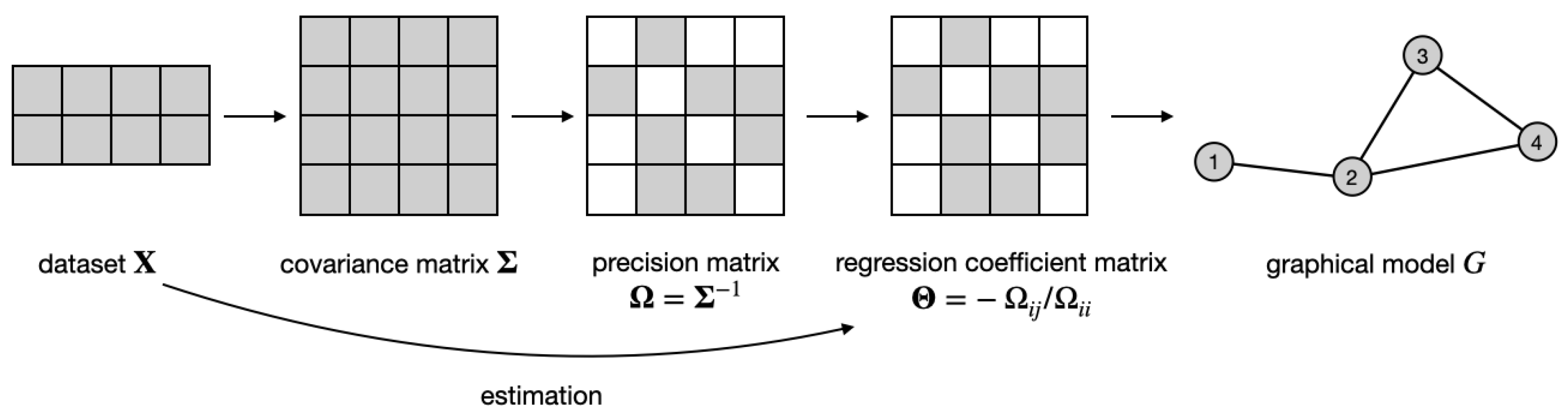
Let ${\mathbf{X}}^{\left(1\right)},{\mathbf{X}}^{\left(2\right)},\dots ,{\mathbf{X}}^{\left(K\right)}$ be $K\ge 2$ datasets containing measurements of (almost) the same variables under K different but similar conditions (e.g., sub-types of disease) or collected in distinct classes (e.g., different equipment or laboratories). Each dataset ${\mathbf{X}}^{\left(k\right)}$ is an $n_k\times p_k$ data matrix with $n_k$ observations of $p_k$ variables. We assume that observations ${({\mathit{x}}_1^{\left(k\right)},\dots ,{\mathit{x}}_{n_k}^{\left(k\right)})}^{\top }$ are independent and identically distributed samples from a $p_k$-variate Gaussian distribution with zero mean and covariance matrix ${\mathsf{\Sigma }}^{\left(k\right)}$.

Every distribution $\mathcal{N}(0,{\mathsf{\Sigma }}^{\left(k\right)})$ is associated with a graphical model $G^{\left(k\right)}=(V_k,E_k)$, where vertices correspond to random variables, i.e., $V_k=\{X_1^{\left(k\right)},\dots ,X_{p_k}^{\left(k\right)}\}$, and the absence of edges (where $E_k\subseteq V_k\times V_k$) implies the conditional independence of the corresponding variables, i.e., $(i,j)\notin E_k\iff X_i^{\left(k\right)}⫫X_j^{\left(k\right)}|X_{\{l,l\ne i,j\}}^{\left(k\right)}$. It is well known that the support of the precision matrix encodes the graph structure, i.e., $(i,j)\in E_k⟺{\mathsf{\Omega }}_{ij}^{\left(k\right)}\ne 0$, where ${\mathsf{\Omega }}^{\left(k\right)}={({\mathsf{\Sigma }}^{\left(k\right)})}^{-1}$ is the true precision matrix for the k-th class. Therefore, for each dataset, the problem of graph estimation becomes equivalent to estimating the support of the precision matrix, as illustrated in Figure 1. However, when the K datasets share some dependency structure (as occurs when we consider similar datasets), a joint inference can be more powerful and accurate, as already shown in [1] and referenced therein. The joint inference requires modeling how the information about the graphs $G^{\left(k\right)}$ is shared across different datasets.

In [1], we proposed the following joint estimation approach. We started with an assumption that although the covariance matrices ${\mathsf{\Sigma }}^{\left(k\right)}$, $k=1\dots K$, might be different, the structures of K graphs coincide, i.e., the graph G is the same across all datasets. Therefore, we needed to estimate the same support from K precision matrices. However, instead of doing that directly, we estimated the support of K regression coefficient matrices. We defined them as ${\mathsf{\Theta }}^{\left(k\right)}\in R^{p_k\times p_k}$ with entries ${\mathsf{\Theta }}_{ij}^{\left(k\right)}=-{\mathsf{\Omega }}_{ij}^{\left(k\right)}/{\mathsf{\Omega }}_{ii}^{\left(k\right)}$ and ${\mathsf{\Theta }}_{ii}^{\left(k\right)}=0$. By construction, the support of the extra-diagonal entries of ${\mathsf{\Theta }}^{\left(k\right)}$ also encodes the graph structure, i.e.,  $(i,j)\in E_k⟺{\mathsf{\Theta }}_{ij}^{\left(k\right)}\ne 0$. 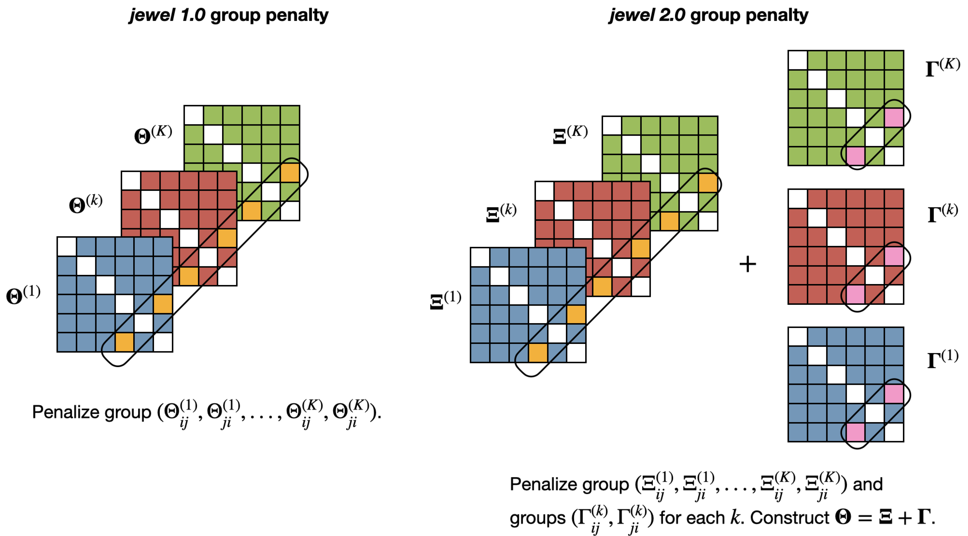Hence, in jewel 1.0, we simultaneously estimated ${\widehat{\mathsf{\Theta }}}^{\left(1\right)},\dots ,{\widehat{\mathsf{\Theta }}}^{\left(K\right)}$ by solving the following minimization problem:

$$\begin{array}{c}\hfill ({\widehat{\mathsf{\Theta }}}^{\left(1\right)},\dots ,{\widehat{\mathsf{\Theta }}}^{\left(K\right)})=\underset{\begin{array}{c}{\mathsf{\Theta }}^{\left(1\right)}\in {\mathbb{R}}^{p_1\times p_1}\\ ⋮\\ {\mathsf{\Theta }}^{\left(K\right)}\in {\mathbb{R}}^{p_K\times p_K},\\ \mathrm{diag}=0\end{array}}{argmin}\{\frac{1}{2}\sum _{k=1}^K{\displaystyle \frac{1}{n_k}}\Vert {\mathbf{X}}^{\left(k\right)}-{\mathbf{X}}^{\left(k\right)}{\mathsf{\Theta }}^{\left(k\right)}{\Vert }_F^2+\\ \hfill \lambda \sum _{i<j=1}^p\sqrt{g_{ij}}\sqrt{\sum _{k:\{X_i,X_j\}\subset V_k}{\left({\mathsf{\Theta }}_{ij}^{\left(k\right)}\right)}^2+{\left({\mathsf{\Theta }}_{ji}^{\left(k\right)}\right)}^2}\},\end{array}$$

(1)

where $g_{ij}$ denotes the cardinality of the group of symmetric variables $({\mathsf{\Theta }}_{ij}^{\left(1\right)},{\mathsf{\Theta }}_{ji}^{\left(1\right)},\dots \dots ,{\mathsf{\Theta }}_{ij}^{\left(K\right)},$ ${\mathsf{\Theta }}_{ji}^{\left(K\right)})$ across all the datasets that contain the couple of variables $(i,j)$. As a result, we obtained K matrices $({\widehat{\mathsf{\Theta }}}^{\left(1\right)},\dots ,{\widehat{\mathsf{\Theta }}}^{\left(K\right)})$ with the same symmetric support, which represents the adjacency matrix of the common estimated graph $\widehat{G}$.

However, while the symmetry of the solution of Equation (1) is one of the main advantages of our original formulation, forcing the datasets to have exactly the same underlying graph might be a limitation in some cases. For example, the assumption that the datasets ${\mathbf{X}}^{\left(k\right)}$, $k=1\dots K$, share the same graph G might be reasonable when they represent the gene expression of the same type of cells, measured in different laboratories or with different instruments. In such cases, we expect the actual underlying regulatory mechanisms to remain the same despite the technology. However, the assumption becomes limited when the datasets represent the gene expression in cells isolated from different sub-types or stages of some disease. In such a context, we expect a common underlying mechanism that can be associated with that disease, but there could be sub-type-specific differences that are not shared across all the datasets but characterize only one (or some, but not all) condition. To overcome this limitation, in this paper, we modify the formulation of the minimization problem in Equation (1) to allow the modeling of both commonalities and differences between the graphs $G^{\left(k\right)}$, $k=1\dots K$. Therefore, by relaxing the assumptions, we increase the range of applications of our approach.

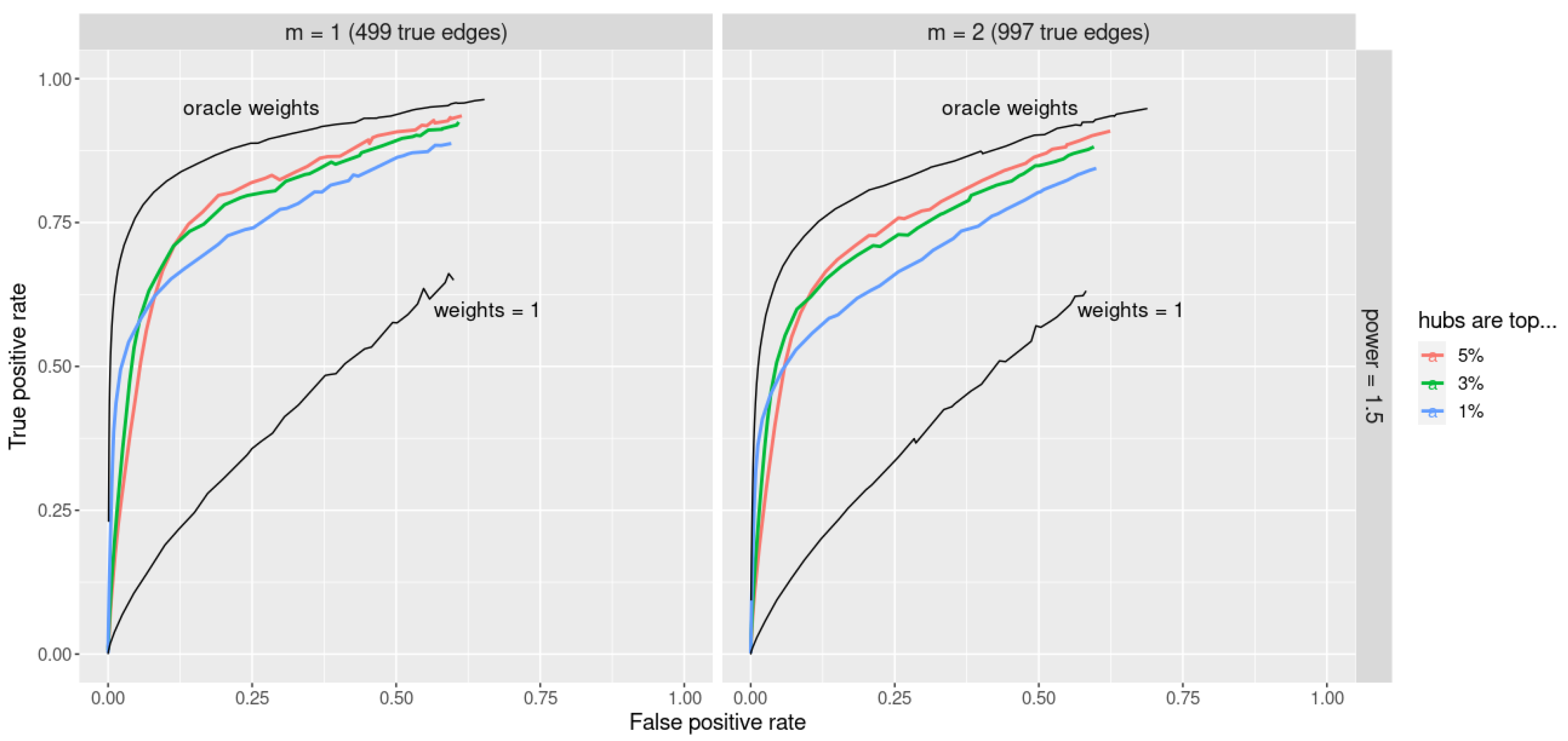
Additionally, in [1] we demonstrated that jewel 1.0 performs comparably well or even better than other joint approaches for GGM (i.e., JGL [4] and the proposal of Guo et al. [5]). However, we also showed that all methods’ performances significantly decreased when the true graph contained hubs. Scale-free graphs with a power of preferential attachment bigger than 1 constitute typical examples of graphs with hubs. In general, many real-life graphs such as gene regulatory networks or protein–protein interaction networks are estimated to have a power law between 2 and 3. Therefore, we introduced some weights into the penalization problem to allow for a better estimation of hubs. The key idea is that small weights must be assigned to the edges linked to potential hubs so that hubs can emerge (in other words, we allow the preferential attachment of an edge to a hub). We will show that this modification leads to a considerable improvement in performance when some preliminary information on the hubs is available. We note that although other graph estimation methods with weighted penalties exist for one dataset, e.g., DW-lasso [6], jewel 2.0 is the first joint method for several datasets with a weighted penalty.

To incorporate both changes, we reformulate the minimization problem as follows. We define the set $V=V_1\cup \cdots \cup V_K$ with p being its cardinality. We define matrices of weights for each graph, ${\mathbf{W}}^{\left(k\right)}$, with entries $W_{ij}^{\left(k\right)}\in (0,1]$. These matrices incorporate information about hubs when available (smaller weights should be assigned to edges incident to hubs, larger weights to the others); otherwise, we set ${\mathbf{W}}^{\left(k\right)}=\mathbf{1}$. For each class $k=1\dots K$ we set ${\mathsf{\Theta }}^{\left(k\right)}={\mathsf{\Xi }}^{\left(k\right)}+{\mathsf{\Gamma }}^{\left(k\right)}$, where matrices ${\mathsf{\Xi }}^{\left(k\right)}$ share the same support structure among the K classes (i.e., they represent the common information shared across different graphs) while ${\mathsf{\Gamma }}^{\left(k\right)}$ are class-specific (hence they allow to model differences among the classes). We emphasize that ${\mathsf{\Xi }}^{\left(k\right)}$ and ${\mathsf{\Gamma }}^{\left(k\right)}$, $k=1\dots K$, act as auxiliary (or dummy) variables and do not exactly represent common and specific parts of the graphs $G^{\left(k\right)}$. For example, non-zero elements in position $i,j$ of all ${\mathsf{\Gamma }}^{\left(k\right)}$ are an indication of the common edge, despite the fact of being present in class-specific ${\mathsf{\Gamma }}^{\left(k\right)}$s. In our procedure, we estimate ${\widehat{G}}^{\left(k\right)}$ through the support of ${\mathsf{\Theta }}^{\left(k\right)}={\mathsf{\Xi }}^{\left(k\right)}+{\mathsf{\Gamma }}^{\left(k\right)}$. Once we have estimated ${\widehat{G}}^{\left(k\right)},k=1\dots K$, we can later identify their common part as the intersection of the estimated graphs and the specific parts as the difference between the common part and the individual estimates. With this notation, we estimate ${\widehat{\mathsf{\Theta }}}^{\left(1\right)},\dots ,{\widehat{\mathsf{\Theta }}}^{\left(K\right)}$ by solving the following problem:

$$\begin{array}{c}\hfill ({\widehat{\mathsf{\Xi }}}^{\left(1\right)},{\widehat{\mathsf{\Gamma }}}^{\left(1\right)},\dots ,{\widehat{\mathsf{\Xi }}}^{\left(K\right)},{\widehat{\mathsf{\Gamma }}}^{\left(K\right)})=\underset{\begin{array}{c}{\mathsf{\Xi }}^{\left(1\right)},{\mathsf{\Gamma }}^{\left(1\right)}\in {\mathbb{R}}^{p_1\times p_1}\\ ⋮\\ {\mathsf{\Xi }}^{\left(K\right)},{\mathsf{\Gamma }}^{\left(K\right)}\in {\mathbb{R}}^{p_K\times p_K},\\ \mathrm{diag}=0\end{array}}{argmin}\{\frac{1}{2}\mathbf{\sum }_{k=1}^K{\displaystyle \frac{1}{n_k}}\Vert {\mathbf{X}}^{\left(k\right)}-{\mathbf{X}}^{\left(k\right)}{\mathsf{\Xi }}^{\left(k\right)}-{\mathbf{X}}^{\left(k\right)}{\mathsf{\Gamma }}^{\left(k\right)}{\Vert }_F^2+\\ \hfill +{\lambda }_1\mathbf{\sum }_{i<j=1}^p\sqrt{g_{ij}}{\overline{W}}_{ij}\sqrt{\mathbf{\sum }_{k:\{X_i,X_j\}\subset V_k}{\left({\mathsf{\Xi }}_{ij}^{\left(k\right)}\right)}^2+{\left({\mathsf{\Xi }}_{ji}^{\left(k\right)}\right)}^2}\\ \hfill +{\lambda }_2\mathbf{\sum }_{i<j=1}^p\sqrt{2}\mathbf{\sum }_{k:\{X_i,X_j\}\subset V_k}{W}_{ij}^{\left(k\right)}\sqrt{{\left({\mathsf{\Gamma }}_{ij}^{\left(k\right)}\right)}^2+{\left({\mathsf{\Gamma }}_{ji}^{\left(k\right)}\right)}^2}\},\end{array}$$

(2)

where ${\overline{W}}_{ij}=1/K{\sum }_k{W}_{ij}^{\left(k\right)}$ and ${\lambda }_1$, ${\lambda }_2$ are two regularization parameters.

Note that the minimization problem in Equation (2) has two penalty terms. The first penalty is applied to the entire group $({\mathsf{\Xi }}_{ij}^{\left(1\right)},{\mathsf{\Xi }}_{ji}^{\left(1\right)},\dots ,{\mathsf{\Xi }}_{ij}^{\left(K\right)},{\mathsf{\Xi }}_{ji}^{\left(K\right)})$ and enforces the presence/absence of an edge across all classes containing that edge (to capture common dependencies). The second penalty is applied independently to each group $({\mathsf{\Gamma }}_{ij}^{(k)},{\mathsf{\Gamma }}_{ji}^{\left(k\right)})$, $k=1\dots K$. This enforces the symmetry of the relation between two nodes in each class, allowing class-specific differences to emerge. Figure 2 provides an illustration of the idea.

Moreover, the weights $W_{ij}^{\left(k\right)}$ in the penalties allow hubs to emerge. By assigning lower weights to edges linked to potential hubs, we reduce the penalty on those edges and allow hubs to emerge. Instead, by choosing $W_{ij}^{\left(k\right)}=1$, we have a more democratic approach that is equivalent to an unweighted formulation. Weights could be estimated from the data or provided by the user from prior knowledge, literature, and databases. Currently, using information already available in the literature (from previous experiments) or knowledge stored in databases is becoming widespread, particularly in omics science, where international projects and consortiums have released an enormous amount of data in open form. For example, in [7], the authors suggested using gene networks retrieved from databases to improve survival prediction. Here, we propose the use of information concerning potential highly influential genes to estimate networks with hubs better. Section 3.2.2 discusses weight choice in detail.

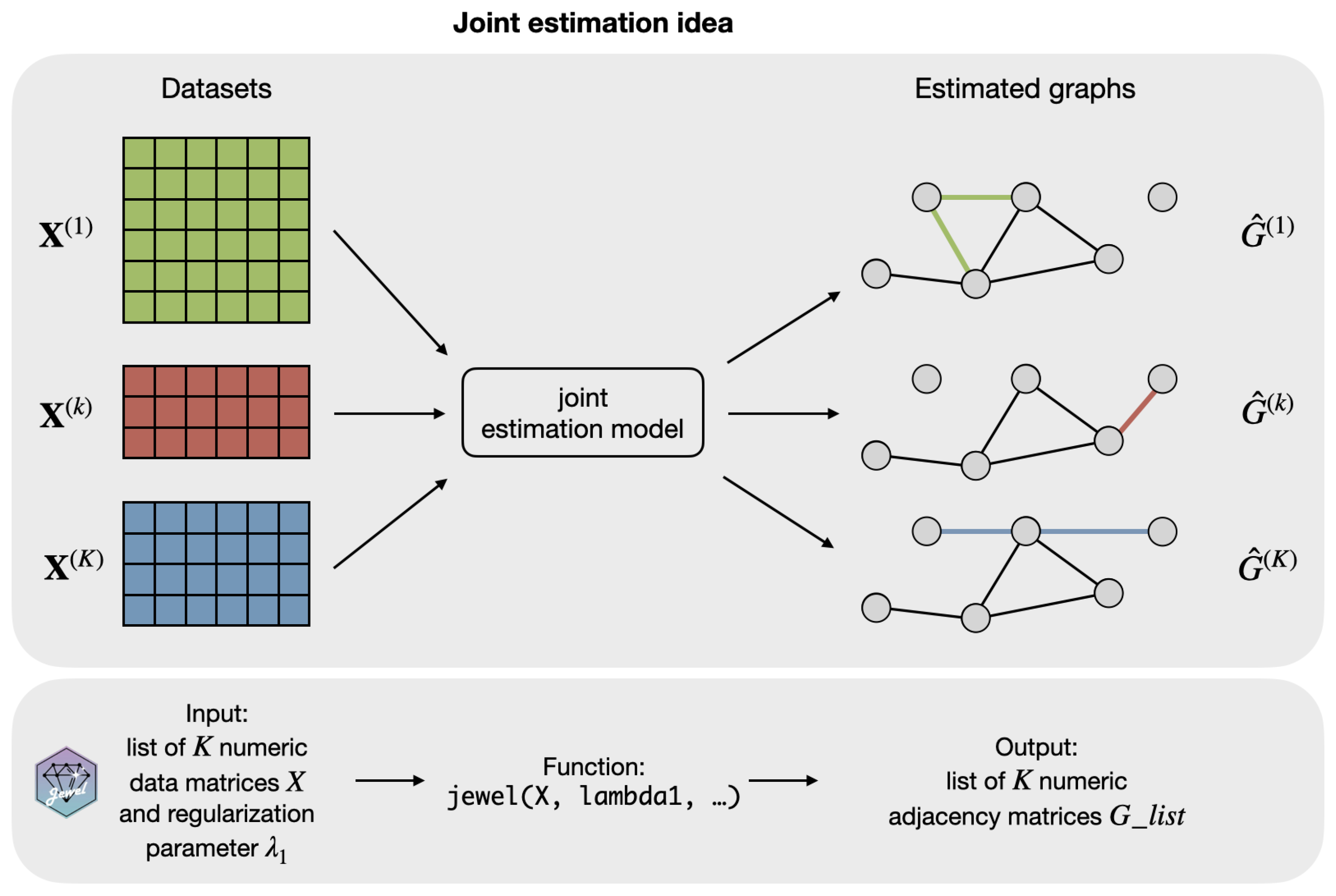
Finally, we note that the minimization problem in Equation (2) is not identifiable in terms of ${\mathsf{\Xi }}^{\left(k\right)}$ and ${\mathsf{\Gamma }}^{\left(k\right)}$ but is identifiable in terms of the support of ${\mathsf{\Theta }}^{\left(k\right)}$, provided that we estimate it using ${\mathsf{\Xi }}^{\left(k\right)}+{\mathsf{\Gamma }}^{\left(k\right)}$. Furthermore, as a result of the minimization problem in Equation (2), we obtain K graphs ${\widehat{G}}^{\left(k\right)}$ with largely the same structure G but also allow some class-specific edges. See Figure 3 for an illustration of the idea.

2.2. Jewel 2.0 Algorithm

To solve the minimization problem in Equation (2), we apply the group descent algorithm presented in [8]. To better describe this algorithm, we rewrite the problem in Equation (2) using an equivalent formulation. To this end, we define the following matrices and vectors (note that for the ease of notation without loss of generality, we suppose $p_1=\cdots =p_K=p$):

-

$X_{.i}^{\left(k\right)}$ the i-th column of matrix ${\mathbf{X}}^{\left(k\right)}$ and ${\mathbf{X}}_{.-i}^{\left(k\right)}$ the submatrix of ${\mathbf{X}}^{\left(k\right)}$ without the i-th column;

-

$\mathit{y}={\left({X_{.1}^{\left(1\right)}}^{\top },\dots ,{X_{.p}^{\left(1\right)}}^{\top },\dots ,{X_{.1}^{\left(K\right)}}^{\top },\dots ,{X_{.p}^{\left(K\right)}}^{\top }\right)}^{\top }$ denotes the vector concatenating the columns of all data matrices, $dim\left(\mathit{y}\right)=Np\times 1$, $N={\sum }_{k=1}^K{n}_k$;

-

$\mathit{\xi }=\left({\mathsf{\Xi }}_{21}^{\left(1\right)},\dots ,{\mathsf{\Xi }}_{p1}^{\left(1\right)},\dots ,{\mathsf{\Xi }}_{1p}^{\left(K\right)},\dots ,{\mathsf{\Xi }}_{(p-1)p}^{\left(K\right)}\right)$, $dim\left(\mathit{\xi }\right)=1\times p(p-1)K$, and 

$\mathit{\gamma }=\left({\mathsf{\Gamma }}_{21}^{\left(1\right)},\dots ,{\mathsf{\Gamma }}_{p1}^{\left(1\right)},\dots ,{\mathsf{\Gamma }}_{1p}^{\left(K\right)},\dots ,{\mathsf{\Gamma }}_{(p-1)p}^{\left(K\right)}\right)$, $dim\left(\mathit{\gamma }\right)=1\times p(p-1)K$,

are obtained by concatenating the vectorized matrices over the K classes;

-

$$\mathbf{X}=\left(\begin{array}{ccc}\left(\begin{array}{cccc}{\mathbf{X}}_{.-1}^{\left(1\right)}& 0& \dots & 0\\ 0& {\mathbf{X}}_{.-2}^{\left(1\right)}& \dots & 0\\ ⋮& & \ddots & \\ 0& \dots & & {\mathbf{X}}_{.-p}^{\left(1\right)}\end{array}\right)& & \\ & \ddots & \\ & & \left(\begin{array}{cccc}{\mathbf{X}}_{.-1}^{\left(K\right)}& 0& \dots & 0\\ 0& {\mathbf{X}}_{.-2}^{\left(K\right)}& \dots & 0\\ ⋮& & \ddots & \\ 0& \dots & & {\mathbf{X}}_{.-p}^{\left(K\right)}\end{array}\right)\end{array}\right)$$

denotes the block-diagonal matrix made up of the block-diagonal matrices ${\mathbf{X}}_{.-j}^{\left(k\right)}$, $k=1\dots K$, $j=1\dots p$, $dim\left(\mathbf{X}\right)=Np\times p(p-1)K$;

-

augmented matrix $\tilde{\mathbf{X}}=\left[\mathbf{X}\mathbf{X}\right]$;

-

diagonal matrix $\mathit{D}=\mathrm{blkdiag}{\left((1/\sqrt{n_k}){\mathit{I}}_{n_{k}p}\right)}_{k=1\dots K}$, $dim\left(\mathit{D}\right)=Np\times Np$.

With these notations, the problem in Equation (2) is equivalent to the following linear regression model with non-overlapping weighted group lasso penalties:

$$(\widehat{\mathit{\xi }},\widehat{\mathit{\gamma }})=\underset{\mathit{\xi },\mathit{\gamma }\in {\mathbb{R}}^{p(p-1)K}}{argmin}\underset{F(\mathit{\xi },\mathit{\gamma })}{\underbrace{\frac{1}{2}{‖\mathit{y}-\tilde{\mathbf{X}}{\left[\mathit{\xi }\mathit{\gamma }\right]}^{\top }‖}_{{\mathit{D}}^2}+{\lambda }_1\sum _{i<j=1}^p\sqrt{g_{ij}}{\overline{W}}_{ij}\Vert {\mathit{\xi }}_{\left[ij\right]}\Vert +{\lambda }_2\sum _{i<j=1}^p\sqrt{2}\sum _k{W}_{ij}^{\left(k\right)}\Vert {\mathit{\gamma }}_{\left[ijk\right]}\Vert .}}$$

(3)

Function $F(\mathit{\xi },\mathit{\gamma })$ in Equation (3) is jointly convex in $\mathit{\xi }$ and $\mathit{\gamma }$, and the two penalties involve $\mathit{\xi }$ or $\mathit{\gamma }$ independently. Hence, we can apply an alternating optimization algorithm as follows:

-

initialize vector $\mathit{\gamma }$;

-

given $\mathit{\gamma }$, estimate $\mathit{\xi }$ by

$$\widehat{\mathit{\xi }}=\underset{\mathit{\xi }\in {\mathbb{R}}^{p(p-1)K}}{argmin}\frac{1}{2}{‖\tilde{\mathit{y}}-\mathbf{X}{\mathit{\xi }}^{\top }‖}_{{\mathit{D}}^2}+{\lambda }_1\sum _{i<j=1}^p\sqrt{g_{ij}}{\overline{W}}_{ij}\Vert {\mathit{\xi }}_{\left[ij\right]}\Vert ,\mathrm{w}\mathrm{i}\mathrm{t}\mathrm{h}\tilde{\mathit{y}}=\mathit{y}-\mathbf{X}{\mathit{\gamma }}^{\top };$$

-

given $\mathit{\xi }$, estimate $\mathit{\gamma }$ by

$$\widehat{\mathit{\gamma }}=\underset{\mathit{\gamma }\in {\mathbb{R}}^{p(p-1)K}}{argmin}\frac{1}{2}{‖\tilde{\mathit{y}}-\mathbf{X}{\mathit{\gamma }}^{\top }‖}_{{\mathit{D}}^2}+{\lambda }_2\sum _{i<j=1}^p\sqrt{2}\sum _k{W}_{ij}^{\left(k\right)}\Vert {\mathit{\gamma }}_{\left[ijk\right]}\Vert ,\mathrm{w}\mathrm{i}\mathrm{t}\mathrm{h}\tilde{\mathit{y}}=\mathit{y}-\mathbf{X}{\mathit{\xi }}^{\top }.$$

The two steps are alternated and repeated until convergence.

Since the groups are non-overlapping and orthogonal by construction, each minimization step can be solved using the group descent algorithm of [8]. Algorithm 1 illustrates the steps of the proposed jewel 2.0 algorithm in details.

Note that Algorithm 1 generalizes the one presented in [1] to the double penalties (which are alternately updated) in the minimization problem in Equation (2). However, it still uses the idea of the Active matrices discussed in [1], where only non-zero entries are updated. The algorithm provided here also has a minor difference compared to the jewel 1.0 version: now, the order of variables is randomized instead of being $1\to p$. Although the algorithm converges regardless of the order [8], we decided to use the random order of updates because we have empirically seen that it provides an advantage in the running time without loss in performance. Finally, we note that the matrices and vectors defined in this subsection to describe the algorithm do not need to be explicitly constructed to implement the algorithm, as discussed in [1].

Algorithm 1 The jewel 2.0 algorithm.

INPUT: data ${\mathbf{X}}^{\left(1\right)},\dots ,{\mathbf{X}}^{\left(K\right)}$, weights ${\mathbf{W}}^{\left(1\right)},\dots ,{\mathbf{W}}^{\left(K\right)}$

parameters ${\lambda }_1$, ${\lambda }_2$, $tol$ and $t_{max}$

INITIALIZE:

Common part: ${\mathsf{\Xi }}^{(1,0)},\dots ,{\mathsf{\Xi }}^{(K,0)}$

Specific part: ${\mathsf{\Gamma }}^{(1,0)},\dots ,{\mathsf{\Gamma }}^{(K,0)}$

Residuals (common and specific): ${\mathit{RC}}^{\left(k\right)}={\mathit{RS}}^{\left(k\right)}={\mathbf{X}}^{\left(k\right)}-{\mathbf{X}}^{\left(k\right)}{\mathsf{\Gamma }}^{(k,0)}-{\mathbf{X}}^{\left(k\right)}{\mathsf{\Xi }}^{(k,0)}$

Matrices of active pairs $\mathbf{Active}={\mathbf{Active}}^{\left(k\right)}=\left(\begin{array}{cccc}0& 1& \dots & 1\\ 0& 0& & 1\\ ⋮& & \ddots & ⋮\\ 0& 0& \dots & 0\end{array}\right)\forall k$

REPEAT UNTIL CONVERGENCE

Fix the specific part ${\mathsf{\Gamma }}^{(1,t)},...,{\mathsf{\Gamma }}^{(K,t)}$, update the COMMON part.

Generate $orde{r}_{\mathsf{\Xi }}$ by resampling from 1 to p.

for$j\in orde{r}_{\mathsf{\Xi }}$ do

for $i=j+1\dots p$ do

if $Activ{e}_{ij}\ne 0$ then

evaluate $\mathit{z}=\left(z_{ij}^{\left(1\right)},z_{ji}^{\left(1\right)},\dots ,z_{ij}^{\left(K\right)},z_{ji}^{\left(K\right)}\right)$ by $$\begin{array}{cc}{z}_{ij}^{\left(k\right)}\hfill & ={\displaystyle \frac{1}{n_k}}{X_{.i}^{\left(k\right)}}^{\top }{RC}_{.j}^{\left(k\right)}+{\mathsf{\Xi }}_{ij}^{(k,t)}\hfill \\ z_{ji}^{\left(k\right)}& ={\displaystyle \frac{1}{n_k}}{X_{.j}^{\left(k\right)}}^{\top }{RC}_{.i}^{\left(k\right)}+{\mathsf{\Xi }}_{ji}^{(k,t)}\hfill \end{array}$$

compute ${\overline{W}}_{ij}={\sum }_k{W}_{ij}^{\left(k\right)}/K$

evaluate $threshold=1-{\lambda }_1\sqrt{g_{ij}}{\overline{W}}_{ij}/\parallel \mathit{z}\parallel$

if $threshold<0$ then

$Activ{e}_{ij}\leftarrow 0$ and $\mathit{z}\leftarrow 0$

else

$\mathit{z}\leftarrow \mathit{z}·threshold$

end if

update residuals $$\begin{array}{cc}\hfill {RC}_{.j}^{\left(k\right)}& ={RC}_{.j}^{\left(k\right)}+X_{.i}^{\left(k\right)}\left({\mathsf{\Xi }}_{ij}^{(k,t)}-z_{ij}^{\left(k\right)}\right)\hfill \\ {RC}_{.i}^{\left(k\right)}\hfill & \hfill ={RC}_{.i}^{\left(k\right)}+X_{.j}^{\left(k\right)}\left({\mathsf{\Xi }}_{ji}^{(k,t)}-z_{ji}^{\left(k\right)}\right)\end{array}$$

update coefficients $({\mathsf{\Xi }}_{ij}^{(1,t+1)},{\mathsf{\Xi }}_{ji}^{(1,t+1)},\dots ,{\mathsf{\Xi }}_{ij}^{(K,t+1)},{\mathsf{\Xi }}_{ij}^{(K,t+1)})\leftarrow \mathit{z}$

end if

end for

end for

Update residuals ${\mathit{RS}}^{\left(k\right)}={\mathbf{X}}^{\left(k\right)}-{\mathbf{X}}^{\left(k\right)}{\mathsf{\Gamma }}^{(k,t)}-{\mathbf{X}}^{\left(k\right)}{\mathsf{\Xi }}^{(k,t+1)}$.

Fix the common part ${\mathsf{\Xi }}^{(1,t+1)},...,{\mathsf{\Xi }}^{(K,t+1)}$, update the SPECIFIC part.

Generate $orde{r}_{\mathsf{\Gamma }}$ by resampling from 1 to p.

for$k=1\dots K$do

for $j\in orde{r}_{\mathsf{\Gamma }}$ do

for $i=j+1\dots p$ do

if $Activ{e}_{ij}^{\left(k\right)}\ne 0$ then

evaluate $\mathit{z}=\left(z_{ij}^{\left(k\right)},z_{ji}^{\left(k\right)}\right)$ by $$\begin{array}{cc}{z}_{ij}^{\left(k\right)}\hfill & ={\displaystyle \frac{1}{n_k}}{X_{.i}^{\left(k\right)}}^{\top }{RS}_{.j}^{\left(k\right)}+{\mathsf{\Gamma }}_{ij}^{(k,t)}\hfill \\ z_{ji}^{\left(k\right)}\hfill & ={\displaystyle \frac{1}{n_k}}{X_{.j}^{\left(k\right)}}^{\top }{RS}_{.i}^{\left(k\right)}+{\mathsf{\Gamma }}_{ji}^{(k,t)}\hfill \end{array}$$

evaluate $threshold=1-{\lambda }_2\sqrt{2}{W}_{ij}^{\left(k\right)}/\parallel \mathit{z}\parallel$

if $threshold<0$ then

$Activ{e}_{ij}^{\left(k\right)}\leftarrow 0$ and $\mathit{z}\leftarrow 0$

else

$\mathit{z}\leftarrow \mathit{z}·threshold$

end if

update residuals $$\begin{array}{cc}\hfill {RS}_{.j}^{\left(k\right)}& ={RS}_{.j}^{\left(k\right)}+X_{.i}^{\left(k\right)}\left({\mathsf{\Gamma }}_{ij}^{(k,t)}-z_{ij}^{\left(k\right)}\right)\hfill \\ {RS}_{.i}^{\left(k\right)}\hfill & \hfill ={RS}_{.i}^{\left(k\right)}+X_{.j}^{\left(k\right)}\left({\mathsf{\Gamma }}_{ji}^{(k,t)}-z_{ji}^{\left(k\right)}\right)\end{array}$$

update coefficients $({\mathsf{\Gamma }}_{ij}^{(k,t+1)},{\mathsf{\Gamma }}_{ji}^{(k,t+1)})\leftarrow \mathit{z}$

end if

end for

end for

end for

Update residuals ${\mathit{RC}}^{\left(k\right)}={\mathbf{X}}^{\left(k\right)}-{\mathbf{X}}^{\left(k\right)}{\mathsf{\Gamma }}^{(k,t+1)}-{\mathbf{X}}^{\left(k\right)}{\mathsf{\Xi }}^{(k,t+1)}$.

Combine common and specific parts ${\mathsf{\Xi }}^{(k,t+1)}+{\mathsf{\Gamma }}^{(k,t+1)}={\mathsf{\Theta }}^{(k,t+1)}$.

Check convergence: stop if ${\displaystyle \frac{{\sum }_k\left|{\mathsf{\Theta }}^{(k,t+1)}-{\mathsf{\Theta }}^{(k,t)}\right|}{{\sum }_k\left|{\mathsf{\Theta }}^{(k,t)}\right|}}<tol$ or $t>t_{max}$.

OUTPUT:

${\widehat{G}}^{\left(k\right)}=supp{\widehat{\mathsf{\Theta }}}^{(k,t^{*})}$, where $t^{*}$ is the last iteration to achieve the convergence.

$\widehat{G}={\cap }_k{\widehat{G}}^{\left(k\right)}$

2.3. Selection of Regularization Parameter

The minimization problem of Equation (2) contains two regularization parameters: ${\lambda }_1$ which penalizes the common part of the graphs, ${\mathsf{\Xi }}^{\left(k\right)}$, $k=1\dots K$, and ${\lambda }_2$ which penalizes the class-specific part of the graphs, ${\mathsf{\Gamma }}^{\left(k\right)}$, $k=1\dots K$. In general, larger values of the parameters provide a more sparse estimator, which can lead to many false negatives. In contrast, small values of regularization parameters result in dense graphs with more false positives and less interpretability. Therefore, the choice of such parameters is crucial for the success of any regularization method. In this context, the two parameters are not independent since edges set to zero in the common part might be included in the class-specific part and vice-versa.

To better explain the interplay relation between ${\lambda }_1$ and ${\lambda }_2$, we first consider the reparametrization proposed in JGL [4], which connects the regularization parameters to two physical parameters ${\omega }_1$ and ${\omega }_2$ representing the sparsity of the graphs and the similarity across graphs in different classes

$$\begin{array}{cc}\hfill \mathrm{sparsity}:{\omega }_1& ={\displaystyle \frac{{\lambda }_1}{\sqrt{2K}}}+{\displaystyle \frac{{\lambda }_2}{\sqrt{2}}}\hfill \\ \hfill \mathrm{similarity}:{\omega }_2& ={\displaystyle \frac{{\lambda }_2/\sqrt{2}}{{\omega }_1}}.\hfill \end{array}$$

With this reparametrization, we have ${\lambda }_1=\sqrt{2K}{\omega }_1(1-{\omega }_2)$ and ${\lambda }_2=\sqrt{2}{\omega }_1{\omega }_2$. The motivation behind this reparameterization is that it is easier to elicit prior information on ${\omega }_1$ and ${\omega }_2$ than on ${\lambda }_1$ and ${\lambda }_2$.

In a more data-driven spirit, Chapter 9.7 of [9] suggests the use of a proportional relation between the two regularization parameters, namely ${\lambda }_2=\varphi {\lambda }_1$. In the specific setting of matrix decomposition in the multivariate regression, the author proposes the following estimate (see Equation (9.7) of [9]):

$$\varphi ={\displaystyle \frac{\sqrt{\mathrm{maximum}\mathrm{size}\mathrm{over}\mathrm{all}\mathrm{groups}}+\sqrt{log(\#\mathrm{groups})}}{\sqrt{log(\#\mathrm{parameters}\mathrm{to}\mathrm{estimate})}}}.$$

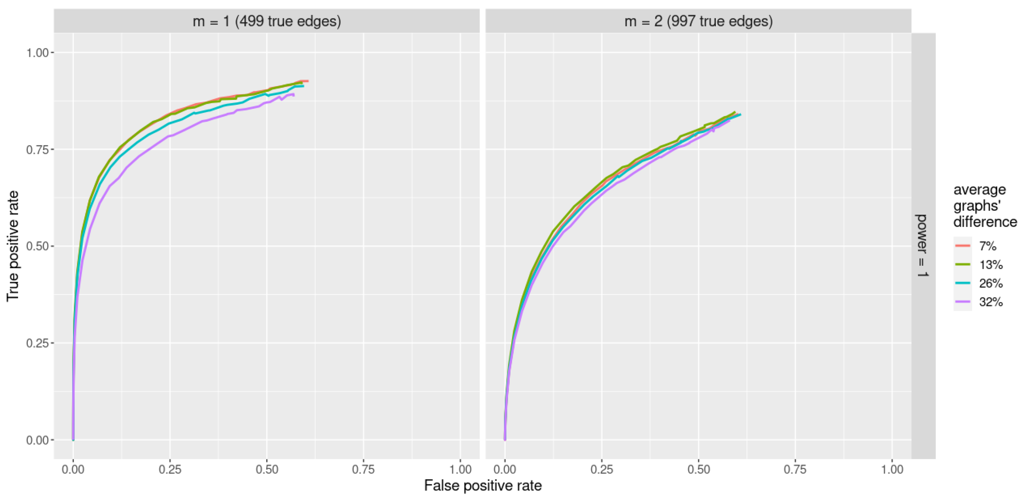
In our case, we still use the relation ${\lambda }_2=\varphi {\lambda }_1$. However, to avoid a computationally intensive data-driven search over $\varphi$, we chose the value $\varphi$ empirically after extensive numerical experimentation under different settings, where we evaluated ROC curves and edges for a range of values $\varphi =1,1.1,1.2,1.3,1.4,1.5$. We set $\varphi =1.4$ (the value that provided the best performance on average among the tested values) and used it in all the subsequent analyses on synthetic and real datasets.

With the established relation ${\lambda }_2=\varphi {\lambda }_1$ and having fixed the value of $\varphi$, the complexity of the parameter space reduces to a choice of only the regularization parameter ${\lambda }_1$. In principle, one can extend the Bayesian information criterion (BIC) as done in [1]. However, there is a long ongoing debate on using BIC in high-dimensional settings. For example, [10] reported poor performance. In general, BIC might be too liberal in the high-dimensional regime. Therefore, the BIC estimate might represent only an empirical rough estimate of the optimal regularization parameter. Its usage beyond empirical evidence would require studying the conditions to guarantee the recovery of the true structure. Since this paper introduces the stability selection procedure (described in the next section), we suggest that the user chooses a value for ${\lambda }_1$ within a plausible range and then applies the stability selection to mitigate the impact on the final estimate of non-optimal choices. We used this suggestion in Section 4. We further discuss the choice of the regularization parameter in Section 5.

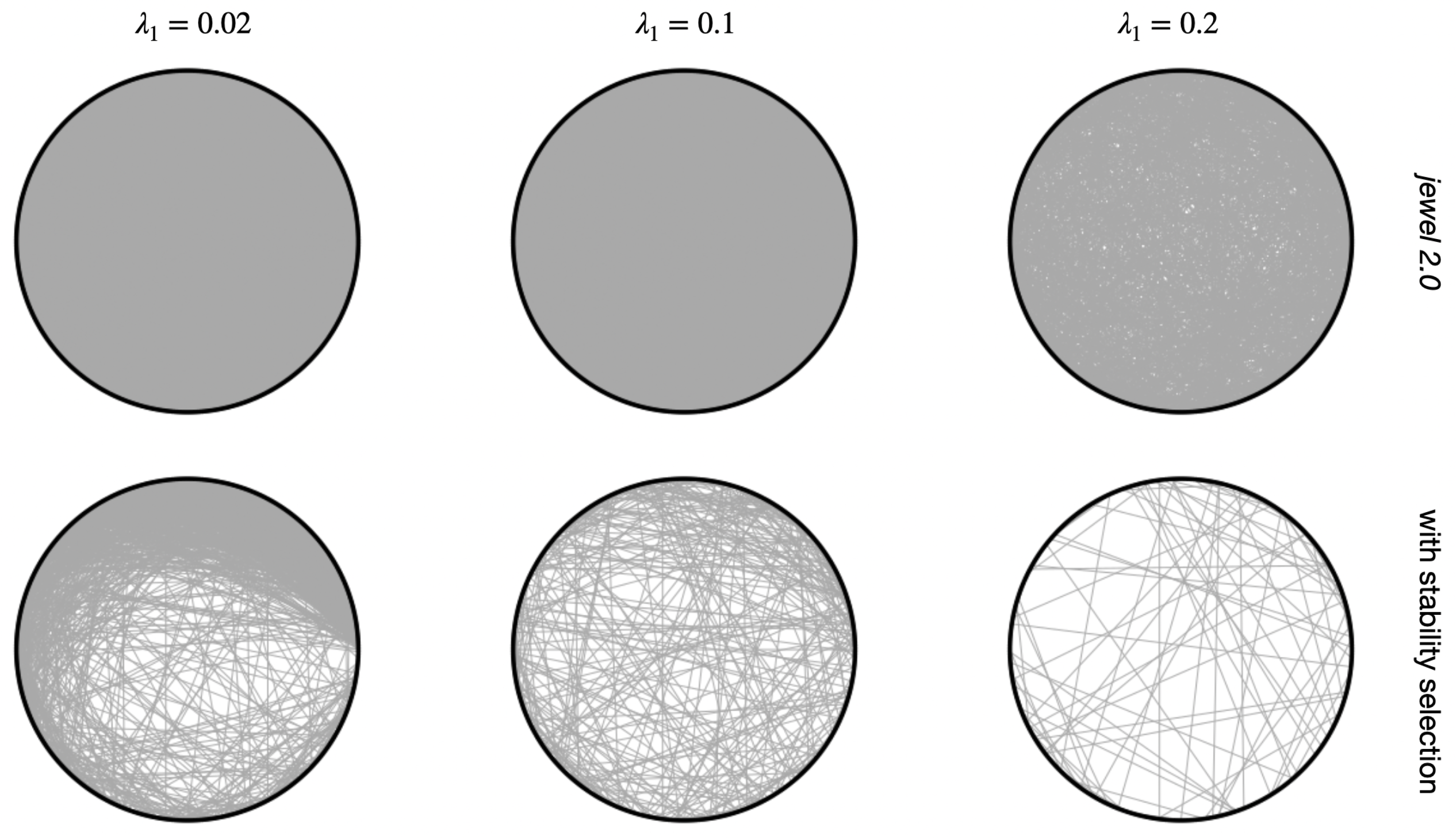
2.4. Stability Selection

Graph estimation can be regarded as a binary classification problem: for each pair of vertices $\{i,j\}$, we decide whether an edge $(i,j)$ exists or not. As with any binary classification method, it is essential to estimate as many true edges as possible and avoid false positives for better interpretability, which becomes especially valuable in high dimensions.

In this respect, another important novelty of jewel 2.0 compared to jewel 1.0 is the implementation of a stable variable selection procedure that decreases the number of false positives. The idea is that actual positive edges should be more stable than false positive edges because the former result from true numerical significance while the latter are merely the result of a chance. With this in mind, one expects that by repeating the calculation several times (on different realizations with a fixed regularization parameter), the true positive edges are more frequent (i.e., appear more stable) than the false positive edges. Motivated by this argument, we extended the idea presented in [3] for the first time to the multiple graphs estimation problem.

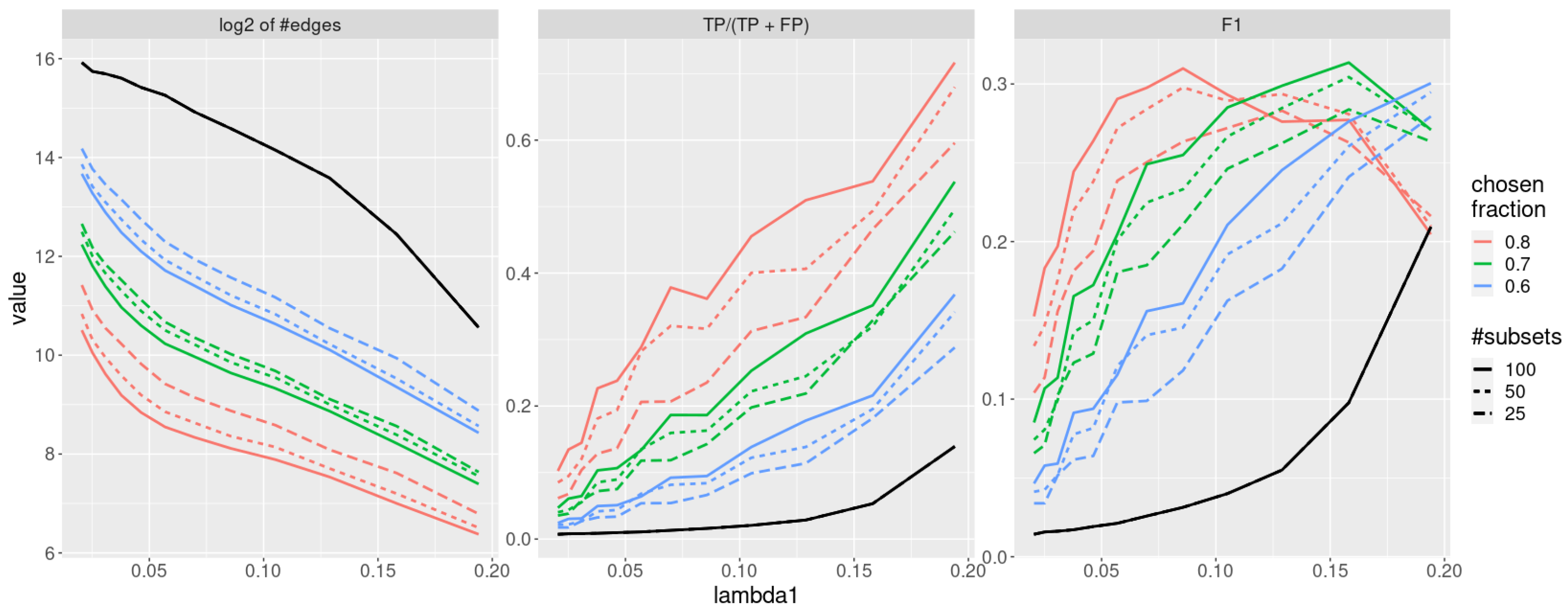
The variable stability selection procedure implemented in jewel 2.0 works as follows. Fix #subsets, representing the number of times we re-run the method on random subsets of the data, and fix chosen fraction, representing the fraction of times that an edge must appear in the results produced on random subsets to be considered stable. Then,

-

Repeat for $s=1\dots$ #subsets

-

randomly subsample the data matrices ${\mathbf{X}}^{(1,s)},{\mathbf{X}}^{(2,s)},\dots ,{\mathbf{X}}^{(K,s)}$ of the size $n_k/2\times p_k$ from ${\mathbf{X}}^{\left(1\right)},{\mathbf{X}}^{\left(2\right)},\dots ,{\mathbf{X}}^{\left(K\right)}$;

-

obtain ${\widehat{G}}^{\left(k\right)}\left(s\right)$, $k=1\dots K$, by applying jewel 2.0 to the subsampled data.

-

Select an edge $\{i,j\}$ in the graph k if $1/\#\mathit{subsets}{\sum }_{s=1}^{\#\mathit{subsets}}Adj({\widehat{G}}_{ij}^{\left(k\right)}\left(s\right)\ne 0)\ge \mathit{chosenfraction}$.

In our approach, the regularization parameter ${\lambda }_1$ is the same throughout the entire stability selection procedure. One might choose, for example, ${\lambda }_1$ obtained with a model selection estimator such as BIC or select a user-defined value (as performed in Section 4) within a reasonable range. The main advantage of the stability selection procedure is that the final estimate of the graphs ${\widehat{G}}^{\left(k\right)}$ is not only sparser but also does not critically depend on the specific choice of the regularization parameter. As we show in the numerical experiment, the stability selection procedure effectively refines the graphs (providing sparser solutions) and reduces the number of false positive edges.

2.5. Code Availability

The jewel 2.0 approach is implemented as an R package jewel, which is freely available at https://github.com/annaplaksienko/jewel (accessed on 15 October 2022). As illustrated in Figure 3, the main function jewel performs the entire algorithm and is relatively simple to use: the user must provide only the list of K numeric data matrices and a numeric value of ${\lambda }_1$, as all other parameters are optional. See package documentation and READ.ME file for the details. All the code to reproduce the simulation studies is provided at https://github.com/annaplaksienko/jewel_simulation_studies (accessed on 15 October 2022).

3. Results on Synthetic Data

This section presents simulation results to demonstrate the specific advantages of jewel 2.0 in handling differences among classes, dealing with network hubs, and refining the networks to reduce false positives and improve interpretability. Moreover, we also compare jewel 2.0 to similar methods for joint Gaussian graphical model estimation. Before presenting the results, in Section 3.1, we briefly describe the data generation procedure for our experimental settings.

3.1. Experimental Settings

To demonstrate the capability of our approach, we used scale-free graphs since they can describe many social and biological processes. Using the following procedure, we generated K scale-free graphs $G^{\left(k\right)}$ with similar supports. We first generated a scale-free graph $G^{\left(1\right)}$ with p vertices with the Barabasi–Albert algorithm [11] (barabasi.game function from the igraph package [12]). We tuned graph sparsity with the m parameter, which describes the number of edges added at each iteration of the Barabasi–Albert algorithm. The resulting graph $G^{\left(1\right)}$ has $mp-(2m-1)$ edges. We monitored the hub structure with the $power$ parameter, which tunes the preferential attachment. With increased power, vertices with more edges are more likely to have new edges to be added to them at each step of the Barabasi–Albert algorithm. Hence, by modifying the $power$ parameter, we can generate networks with different hub/not-hub structures.

Then, given the graph $G^{\left(1\right)}$, we modified it $K-1$ times (to obtain K graphs total) with igraph’s function rewire(..., with = keeping_degseq), which moves the edges of a given graph, preserving its order and the degree distribution. We tuned the number of differences introduced in each modified graph using the $niter$ parameter, i.e., the number of iterations of the algorithm (unless stated otherwise, parameter $niter=0.08\ast p$, making the graphs have about 26% of edges not in common, i.e., not in the intersection).

We used the resulting graphs $G^{\left(k\right)}$, $k=1\dots K$, as the support to construct the precision matrices ${\mathsf{\Omega }}^{\left(k\right)}$. We considered the adjacency matrices of the graphs and replaced all 1s with realizations from the uniform distribution on $[-0.8,-0.2]\cup [0.2,0.8]$. To ensure positive definiteness of ${\mathsf{\Omega }}^{\left(k\right)}$, we set its diagonal elements equal to $|{\mu }_{min}({\mathsf{\Omega }}^{\left(k\right)})|+0.1$, with ${\mu }_{min}$ being the minimum eigenvalue of the matrix. Then, we constructed covariance matrices ${\mathsf{\Sigma }}^{\left(k\right)}$ as ${\Sigma }_{ij}^{\left(k\right)}=({\mathsf{\Omega }}^{\left(k\right)}{)}_{ij}^{-1}/\sqrt{{\left({\mathsf{\Omega }}^{\left(k\right)}\right)}_{ii}^{-1}{\left({\mathsf{\Omega }}^{\left(k\right)}\right)}_{jj}^{-1}}.$ Finally, we generated data matrices ${\mathbf{X}}^{\left(k\right)}$ as $n_k=n$ independent identically distributed observations from $\mathcal{N}(0,{\mathsf{\Sigma }}^{\left(k\right)})$.

In our experimental setting, we chose $K=3$, $p=500$, and $n=100$, and we repeated the above procedure 20 times. We evaluated the performance using the true positive rate $TPR=TP/(TP+FN)$ and false positive rate $FPR=TN/(TN+FP)$, where $FP$ is the number of false positives, $TP$ the number of true positives, $FN$ the number of false negatives, and $TN$ the number of true negatives. jewel 2.0 returns as an output K graphs ${\widehat{G}}^{\left(k\right)}$, instead of the single graph $\widehat{G}$ obtained from jewel 1.0. Therefore, we first calculated $TP{R}^{\left(k\right)}$ and $FP{R}^{\left(k\right)}$ for each graph and then calculated $TPR$ and $FPR$ by averaging over $K=3$ graphs. Finally, we averaged the results over 20 independent runs.

Simulations were carried out on an 8-core 4.2 GHz processor and 32 GB RAM computer.

3.2. Performance of Jewel 2.0

This section aims to illustrate the three main novelties we have introduced with this work. First, we demonstrate the performance of jewel 2.0 when graphs $G^{\left(k\right)}$ have varying amount of differences. Then, we deal with graphs with a non-uniform edge distribution (i.e., graphs with hubs). Finally, we demonstrate how stability selection can reduce the number of false positives and lead to more interpretable graphs.

3.2.1. Performance on Graphs with Varying Differences

We motivated the minimization problem in Equation (2) by the need to estimate graphs $G^{\left(k\right)}$ that share a common part but can have class-specific differences. Therefore, here, we evaluated the performance of jewel 2.0 when applied to datasets with varying differences between their underlying graphs $G^{\left(k\right)}$.

We set the parameter $niter$ in the rewire(..., with = keeping_degseq(niter)) function to $2,4,8,10\%$ of number of vertices p, resulting in graphs with 7, 13, 26, and 32% of difference (on average over 20 independent runs). Here, by “difference” we mean “#edges not in the intersection of $K=3$ graphs”.

ROC curves obtained with the jewel 2.0 method applied to $K=3$ datasets of the size $p=500,$$n_k=100$ and varying underlying graphs are reported in Figure 4. We set the parameter $power=1$, and we compare two different sparsity scenarios: with parameter $m=1$, i.e., 499 edges, and $m=2$, i.e., 997 edges. Here, we set weights $W_{ij}^{\left(k\right)}=1$ regardless of the graph structure.

As we can observe from Figure 4, jewel 2.0 demonstrates good performances in all scenarios of varying amounts of differences between K graphs. Unsurprisingly, the performance decreases as the graphs become increasingly different, but even for 32% of difference, the method still performs well.

3.2.2. Performance on Graphs with Hubs

In [1], we have noticed that the performance of our previous method jewel 1.0 and similar joint estimation methods deteriorates with the increase in the power decay of the degree distribution (i.e., for graphs that contain a few nodes with a significant number of connections and most of the nodes with limited connections). The problem was already noticeable in our simulations for $power=1.5$. To face this problem, in this work, we introduced weights $W_{ij}^{\left(k\right)}$ into the model formulation of Equation (2), whose idea is to adjust the penalty on edge $(i,j)$ according to the degree of its incident nodes i and j. When i and/or j have a high degree, the penalty on the groups involving $\{i,j\}$ is decreased to favor the edge $(i,j)$ to emerge, whereas when i and j have a low degree, the penalty is increased to favor the removal of the edge $(i,j)$.

We first describe an ideal procedure to demonstrate the advantages of our weighted approach by using oracle weights obtained from the true degrees of the nodes, which, of course, are not available in real data applications.

Suppose an oracle provides a vector of true degrees for each class $k=1\dots K$ and denote it ${\mathit{d}}^{\left(k\right)}\in {\mathrm{N}}^p$, with $\mathrm{N}=\{0,1,2,3\dots \}$. We then define the oracle weights matrix ${\mathbf{W}}^{\left(k\right)}$ for the class $k=1\dots K$ by the following formulae:

$${\mathbf{W}}^{\left(k\right)}={\mathbf{W}}^{\left(k\right)}/max({\mathbf{W}}^{\left(k\right)}),with{W}_{ij}^{\left(k\right)}={\displaystyle \frac{1}{\sqrt{d_i^{\left(k\right)}·d_j^{\left(k\right)}}}}.$$

(4)

Note that the re-scaling by $max({\mathbf{W}}^{\left(k\right)})$ assures that weights are in the interval $(0,1]$ and are not dependent on the number of nodes p. Figure 5 (upper black lines) demonstrates that with the oracle choice of weights jewel 2.0 provides excellent performance. In particular, the oracle weights provide a great improvement compared to the no-weight approach (i.e., ${\mathbf{W}}^{\left(k\right)}=\mathbf{1}$, lower black lines in Figure 5).

According to the results of the oracle estimator, we might suggest the use of a two-step procedure where one first applies jewel 2.0 with ${\mathbf{W}}^{\left(k\right)}=\mathbf{1}$ and then estimates the degree vectors ${\widehat{\mathit{d}}}^{\left(k\right)}$, $k=1\dots K$, and reapplies jewel 2.0 using ${\widehat{\mathbf{d}}}^{\left(k\right)}$ as an oracle. However, such a procedure becomes time consuming (since it requires running jewel 2.0 twice) and does not show the same excellent performance as the oracle estimator.

In the spirit of proposing a practical procedure, we noticed that to retain good performance, it is not necessary to know precisely the weights $W_{ij}^{\left(k\right)}$ as given in Equation (4), but it is sufficient to distinguish potential hubs from other nodes. Furthermore, in many applications, it is reasonable to assume that we have prior information on whether or not specific nodes are hubs (but it is less feasible to have prior information on the node degrees). For example, in protein–protein interaction networks, the key players are known from the literature, so we can assume that these nodes are hubs without knowing the exact degree. To evaluate whether a simple procedure is effective, we performed the following simulation:

-

for each k, we considered the vector of true nodes’ degrees ${\mathit{d}}^{\left(k\right)}$;

-

for each k, we fixed a threshold $cu{t}^{\left(k\right)}$ as to choose only a top % of all degrees;

-

if $d_i^{\left(k\right)}>=cu{t}^{\left(k\right)}$, then replace it with 10 (to identify it as a “hub”); else, replace it with 1 (to identify it as “not hub”);

-

finalize weights construction as in Equation (4).

We have evaluated this procedure for choosing weights by setting $cu{t}^{\left(k\right)}$ to select $1,3,5\%$ of the highest degree vertices as ”hubs” for each k. Results are reported in Figure 5 with different colors, as well as the results obtained using ${\mathbf{W}}^{\left(k\right)}=\mathbf{1}$ and the oracle weights.

Figure 5 shows the performance for the power of preferential attachment $power=1.5$. We can see that although the simple procedure is unable to reach the performance of the oracle weights, it outperforms the standard unweighted approach (i.e., ${\mathbf{W}}^{\left(k\right)}=\mathbf{1}$). Moreover, results are quite robust to the percentage of nodes identified as hubs. Results are also robust to the specific value assigned to the hubs (data not shown). Indeed, we applied the same simple procedure assigning 3 or 5 to the hubs instead of 10 and obtained a similar conclusion. Therefore, although an optimal choice of the weights is still needed, the weighted approach proposed in Equation (2) can face the problem of graphs with hubs representing the Achilles’ heel of most of the available methods.

3.2.3. Stability Selection Reduces the Number of False Positives

In this section, we compare the results obtained by running jewel 2.0 on the same dataset without the stability procedure and with the stability procedure described in Section 2.4 where we fixed $\#\mathit{subsets}=25,50,100$ and $\mathit{chosenfraction}=0.6,0.7,0.8$. The results are shown in Figure 6 with different colors and line types. In particular, in the left panel of Figure 6, we show the average (over $K=3$) order of the estimated graphs ${\widehat{G}}^{\left(k\right)}$ (i.e., ${log}_2$ of the average number of estimated edges) as a measure of graph’s “sparseness”; in the middle panel of Figure 6, we show the average precision to measure the proportion of true positive edges, while in the right panel of Figure 6, we show the average F1-score, defined as $F1=2TP/(2TP+FP+FN)$, to measure the overall accuracy. As we can observe from the inspection of Figure 6, the “sparseness” of the estimated graphs decreases with the stability procedure, as expected. More importantly, the stability selection procedure reduces the number of false positives at a much higher rate than the loss of true positives. Overall, it increases the precision (middle panel), maintaining a good accuracy (right panel). We also note that the gain in performance is obtained even with $\#\mathit{subsets}=25$, meaning that stability selection can be used even when a high number of re-sampled sets is not computationally feasible.

To highlight the advantage of having more precise estimates with the same accuracy, i.e., estimated graphs with greater “sparseness”, in Figure 7, we compared results with and without stability selection for the same graph. It is evident that the stability selection estimates sparser graphs than those obtained without stability selection. Comparison is provided for $\#\mathit{subsets}=25$ and $\mathit{chosen\; fraction}=0.8$. Figure 7 is a part of a more extensive comparison on a finer grid of ${\lambda }_1$. When considering the entire study, we also observed that stability makes the final graph estimates less influenced by the specific choice of ${\lambda }_1$. To conclude this subsection, we note that although the idea of the stability selection procedure is not novel, to our knowledge, jewel 2.0 is the first joint estimation method to adopt it in the context of multiple graphs.

3.3. Comparison of Jewel 2.0 with Other Joint Estimation Methods

In this subsection, we compare the performance of jewel 2.0 with other methods for joint estimation: joint graphical lasso (JGL) with group penalty [4], and the proposal of Guo et al. [5]. JGL requires two tuning parameters ${\lambda }_1$ and ${\lambda }_2$, where the first controls for differences between the graphs and the second for graph sparsity. The authors suggested the use of the relation ${\lambda }_1=(1-{\omega }_2)/\left(\sqrt{2}{\omega }_2\right)·{\lambda }_2$. We set parameter ${\omega }_2=0.7$ since it provides better performances in the original paper. Hence, here, we vary only their parameter ${\lambda }_2$.

We also compared jewel 2.0 with another joint estimation method, simone [13] (which, as discussed in [1], is the most similar to jewel 2.0), but we did not include the results in the full comparisons for the following technical reasons. When we provided the range of $\lambda$ parameters from 1 to 0.01 to the simone function, the estimation produced “out of convergence” results for $\lambda \approx 0.15$ or lower (depending on the dataset realization). Using the default function parameters, the simone function went out of convergence even faster. This behavior did not allow us to produce a meaningful ROC curve for [13]. We should note that our simulation settings are different from the ones considered in [13], where the number of variables p was lower, and the authors explored only the $n>p$ setting.

We considered four different $m-power$ scenarios, with parameter $m=1,2$ (resulting in 499 edges with 0.4% sparsity and 997 edges with 0.8% sparsity, respectively, the same settings as we had in all previous experiments) and parameter $power=1,1.5$. In the case of $power=1.5$, we also added jewel 2.0 with a priori weights to the comparison to demonstrate its advantage. In that case, we estimated the weights using the simple approach where we chose 1% of vertices as hubs—even though the performance with this setting was slightly worse than with 3% or 5%, we deemed this one more realistic. Figure 8 illustrates the results of the comparison study.

As we can see in Figure 8, jewel 2.0 and JGL demonstrate similar performance in the case of $power=1$, both superior to the performance of the proposal of Guo et al. As already observed, in the case $power=1.5$, the performance of all three methods drops drastically; however, once we use jewel 2.0 with a simple choice of weights, we see a significant gain in performance. Note that neither $JGL$ nor Guo et al. include methods for dealing with hubs. Therefore, while jewel 2.0 can adapt its penalization to allow hubs to emerge, the other methods remain democratic in their penalization and do not perform well when graphs have hubs.

4. Results on Real Data

The estimation of multiple GGMs could be useful in various contexts. For instance, GGMs allow connections to be found between stocks’ prices (considering different markets as K classes) or social relations (considering different social media as K classes), and so on. In the context of estimating gene networks from gene expression, we can consider gene expression data obtained from different equipment or laboratories (as we did, for example, for jewel 1.0 [1]), or we can consider different sub-types of disease. Identifying the gene regulatory networks and differences associated with a particular sub-disease can help to tailor treatments. Since this paper discusses the advantages of our algorithm from a methodological point of view, in the following, we provide only a small example of an application to real data without investigating the biological implications of our findings.

We apply jewel 2.0 to the gene expression datasets of the patients with breast cancer, which is the most common type of cancer among women. We consider four molecular breast cancer sub-types: luminal A, luminal B, basal-like, and HER2-enriched. Each sub-type can have specific regulatory mechanisms. However, most of the regulatory mechanisms are shared across all sub-types.

We used the gene expression microarray data available in The Cancer Genome Atlas and described in [14]. Gene expressions were measured using Agilent G450 microarrays. The dataset contains 522 primary tumor samples among which there are $n_1=231$ samples of luminal A cancers, $n_2=127$ of luminal B cancers, $n_3=98$ of basal-like cancers, and $n_4=58$ of HER2-enriched cancers. These $K=4$ sub-types were identified in the original paper of [14]. We used the data with $K=4$ datasets to reveal sub-type-specific gene regulatory networks.

For the sake of simplicity, we limited our attention to the genes belonging to the following 10 pathways from the Kyoto Encyclopedia of Genes and Genomes database [15]: breast cancer pathway (hsa05224), estrogen signaling pathway (hsa04915), p53 signaling pathway (hsa04115), PI3K-Akt signaling pathway (hsa04151), GnRH signaling pathway (hsa04912), PPAR signaling pathway (hsa03320), Wnt signaling pathway (hsa04310), NF-kappa B signaling pathway (hsa04064), notch signaling pathway (hsa04330), and hedgehog signaling pathway (hsa04340). According to the literature, these pathways are associated with breast cancer. These pathways involve 945 genes; out of them, 901 were measured in our datasets (with $p=900$ also annotated in the STRING database [16], see below). Therefore, we applied jewel 2.0 (with weights for hub detection and with stability selection) to the $K=4$ submatrices with this subset of genes.

We retrieved prior weights information by building a broad network using the STRING database [16] with $p=900$ genes. STRING is a database of known and predicted protein–protein interactions that can be physical and functional and derived from lab experiments, known co-expression, and genomic context predictions and knowledge in the text mining of the databases. We limited the query to connections from “experiments” and “databases” as active interaction sources and set the minimum required interaction score to the highest value of 0.9. As a result, the STRING network had 775 out of 900 vertices connected to any other node (i.e., 125 nodes were isolated) and 7514 edges.

From the STRING network, we chose the 27 vertices (3% of $p=900$) with the highest true degrees as “hubs”. Therefore, in jewel 2.0, we set their degree to 10 while the degree of all the other vertices was set to 1. We then computed edges’ weights with the Equation (4) formula. We chose regularization parameter empirically as ${\lambda }_1=0.35$. We then ran jewel 2.0 with this parameter, estimated weights, and performed a stability selection procedure with 25 subsets, choosing edges that appeared in at least 80% of the results. The resulting networks are presented in Figure 9.

The resulting networks ${\widehat{G}}^{\left(k\right)}$, $k=1\dots 4$, had 3336, 3297, 3318, and 3313 edges, respectively. There were 3171 edges in their intersection (gray edges in Figure 9, i.e., about 4–6% of edges in each graph were class-specific). For each estimated network, we measured the number of edges in common with the STRING database network and observed 418, 417, 408, and 412 edges in common, respectively. The p-values of the hypergeometric test to assess the significance of the edge overlaps were strictly less than ${10}^{-10}$ for all four networks. Therefore, the estimated graphs showed a significant overlap with the STRING networks compared to random graphs of the same size. This result encourages the quality of the connection, although we also note that connections in the STRING database are not tissue or disease-specific and are not necessarily of the same nature as the ones estimated with jewel 2.0 (conditional dependence). Thus, we did not regard a considerable overlap as the main quality criteria.

We observe that for each of the K estimated graphs, the nodes with the highest degree include the 27 vertices we initially provided as potential hubs. Some of them are key genes in breast cancer, such as LCK, which was shown to influence cell motility in breast cancer, or TRAF6, which promotes tumorigenesis.

Finally, to investigate the impact of the choice of the regularization parameter, we repeated the analysis with a different value (e.g., ${\lambda }_1=0.3$), reporting similar results in terms of estimated networks.

5. Discussion

The proposed method represents a significant advancement of our original method jewel, presented in [1]. jewel 2.0 extends the range of applications by relaxing the assumptions and also provides several other improvements. Namely, by reformulating the minimization problem as in Equation (2), i) jewel 2.0 allows us to jointly estimate both common and class-specific parts of GGMs from multiple datasets, and ii) it allows the user to specify weights to capture the graph topologies that present hubs better. Moreover, with jewel 2.0, we introduced a stability selection procedure to the multiple joint graphical model context. This procedure extends the idea of [3]. It reduces the number of false positives, providing sparser and more explicative graphs, and reduces the influence of the specific choice of the regularization parameter on the estimated graphs. Finally, we demonstrated the performance of jewel 2.0 in simulation and with real data applications.

Although we showed that jewel 2.0 performs well, we believe there is still room for further improvement. Therefore, in the following, we emphasize our study’s limitations and the directions of future work. Furthermore, we stress that limits are not specific to our approach but represent common challenges to all methods available in this context.

The jewel 2.0 minimization problem requires two regularization parameters: ${\lambda }_1$ and ${\lambda }_2$. The choice of the regularization parameters is known to impact the estimator’s performance. In general, under high-dimensional settings, the problem of finding suitable estimates of the regularization parameters is still open, with limited theoretical results available for guaranteeing the recovery of the true structure given the chosen parameter. In this paper, we chose to reduce the complexity of the space by setting ${\lambda }_2=\varphi {\lambda }_1$, fixing $\varphi$ to a default value (selected to produce good performance under different settings). The value of ${\lambda }_1$ can be either estimated from the data (e.g., using BIC or similar data-driven criteria) or chosen by the user in a plausible range of values. In simulations, we investigated the performance of jewel 2.0 when using the ROC curve over a wide range of ${\lambda }_1$. In the real data example, we chose ${\lambda }_1$ empirically and then used the stability selection to reduce the impact of the choice on the final estimate. However, a data-driven estimation of ${\lambda }_1$ or both $\varphi$ and ${\lambda }_1$ would better adapt to the specific data structure. The work of [17] provides an interesting suggestion in this direction.

Another direction of future work consists of improving the stability selection procedure. Inspired by [3], we were the first to introduce a stability selection approach to reduce false positives in the context of multiple graphical model estimation. However, in this context, one can consider further adapting the idea of [3] for setting the bound on the number of false positives or extending the idea of [10]. Both methods used the graphical lasso on a single dataset. Hence, their adaptation to regression-based approaches and multiple datasets might not be straightforward. In general, the study of convergence properties of the resulting estimator would be advisable.

With the weighted approach, we have demonstrated the great improvement that jewel 2.0 can bring when dealing with graphs containing hubs. In several applications, such as gene networks, knowledge available from the literature might give an indication of which genes can act as hubs. The incorporation of this information in the weights improves the estimate. However, the choice of optimal weights remains an open challenge to be addressed in future works.

Finally, the computational cost of GGMs methods on big data remains challenging. Both jewel 1.0 and jewel 2.0 perform well for a number of variables p of the order of several hundreds. Both become unfeasible when applied to tens or hundreds of thousands of variables that might arise from big data analysis. In [1], we showed that other similar methods suffer from the same problem (some more than others), with our approach being the fastest. Although we have introduced some speed-ups (such as the active shooting approach, for example), we believe there is still much room for improvement.