Article

Approximation and Analysis of Natural Data Based on NARX Neural Networks Involving Wavelet Filtering

1
Institute of Cosmophysical Research and Radio Wave Propagation, Far Eastern Branch of the Russian Academy of Sciences, Mirnaya St., 7, Kamchatskiy Kray, 684034 Paratunka, Russia
2
Laboratory of Big Data Technologies in Socio-Cyberphysical Systems, Saint-Petersburg Federal Research Centre of the Russian Academy of Sciences, 199178 St. Petersburg, Russia
3
Department of Technologies of Artificial Intelligence in Physiology and Medicine, Alexander Popov International Innovation Institute for Artificial Intelligence, Cybersecurity and Communications, St. Petersburg State Electrotechnical University “LETI”, 197022 St. Petersburg, Russia
*
Author to whom correspondence should be addressed.
Mathematics 2022, 10(22), 4345; https://doi.org/10.3390/math10224345
Submission received: 12 October 2022 / Revised: 15 November 2022 / Accepted: 17 November 2022 / Published: 19 November 2022
(This article belongs to the Special Issue Statistical Data Modeling and Machine Learning with Applications II)

Abstract

:
Recurrent neural network (RNN) models continue the theory of the autoregression integrated moving average (ARIMA) model class. In this paper, we consider the architecture of the RNN with embedded memory—«Process of Nonlinear Autoregressive Exogenous Model» (NARX). Though it is known that NN is a universal approximator, certain difficulties and restrictions in different NN applications are still topical and call for new approaches and methods. In particular, it is difficult for an NN to model noisy and significantly nonstationary time series. The paper suggests optimizing the modeling process for a complicated-structure time series by NARX networks involving wavelet filtering. The developed procedure of wavelet filtering includes the application of the construction of wavelet packets and stochastic thresholds. A method to estimate the thresholds to obtain a solution with a defined confidence level is also developed. We introduce the algorithm of wavelet filtering. It is shown that the proposed wavelet filtering makes it possible to obtain a more accurate NARX model and improves the efficiency of the forecasting process for a natural time series of a complicated structure. Compared to ARIMA, the suggested method allows us to obtain a more adequate model of a nonstationary time series of complex nonlinear structure. The advantage of the method, compared to RNN, is the higher quality of data approximation for smaller computation efforts at the stages of network training and functioning that provides the solution to the problem of long-term dependencies. Moreover, we develop a scheme of approach realization for the task of data modeling based on NARX and anomaly detection. The necessity of anomaly detection arises in different application areas. Anomaly detection is of particular relevance in the problems of geophysical monitoring and requires method accuracy and efficiency. The effectiveness of the suggested method is illustrated in the example of processing of ionospheric parameter time series. We also present the results for the problem of ionospheric anomaly detection. The approach can be applied in space weather forecasting to predict ionospheric parameters and to detect ionospheric anomalies.
MSC:
62C12; 62C20; 62L20; 68T05; 68T07

1. Introduction

Time series modeling and analysis form an important fundamental basis for the investigation of processes and phenomena of different nature. This theory can be applied in different spheres of human activities (physics, biology, medicine, economy, etc.). A separate class of problems of time series analysis is directed on the diagnostics of object states and anomaly detection. Such problems have special relevance in the area of geophysical monitoring, they are: anomaly detection in geological medium [1]; in the near-earth space [2,3,4]; the prediction of tsunamis [5,6], earthquakes [7], and other catastrophic natural phenomena. Anomaly detection and identification are also very topical in medicine [8]. The most important requirements for such methods are accuracy, promptness of answer reception, as well as the adaptability to have the possibility to record fast nonstationary changes of the system or object state.
Natural data time series have a complex structure that complicates the process of construction of analysis models and methods. Classical methods of time series analysis (AR, ARMA models [9,10], stochastic approximation [11,12], etc.) do not allow us to describe data complex structures adequately, and do not satisfy the adaptation requirement [3,13]. In applications, hybrid approaches are increasingly frequently used. They are based on the combination of deterministic and stochastic methods involving elements of machine learning [3,13,14,15,16,17,18,19]. They allow us to improve the procedure of complex data analysis. For example, in the paper [15], simplified selection ensembles based on trees were used to model and predict the data on milk yield. Preliminary data processing included their reduction into rotating main components. The authors [15] developed a simplified selective algorithm on the index of concordance that allowed them to optimize the method’s performance. In the paper [15], two linear hybrid models were constructed and investigated. Another hybrid approach is considered in the paper [13] to analyze hydrological data. The authors of the paper [13] showed the efficiency of the joint application of wavelet transform [20,21,22] with neural networks (NN): wavelet neural network models. A flexible apparatus of the wavelet transform made it possible to apply it successfully in data analysis application [2]. A set of wavelet decomposition schemes and a wide library of basic wavelets allow us to adapt this method for the data of different-structure and according to the investigation’s aim. The authors of the papers [23,24] illustrated the efficiency of application of wavelet transform with ARIMA models to model ionospheric parameter time variations and to detect anomalies. This paper continues that work. Here, we use the combination of wavelet packets with recurrent neural networks (RNN) [25], which continue the theory of the autoregression integrated moving average (ARIMA) model class [9,10].
Neural network methods are widely applied now in different areas of experience [3,4,7,13,26,27]. However, we should note that NN efficiency depends on the properties of training data and their representativity. Though the NN apparatus includes a wide set of paradigms and allows us to approximate complicated dependencies, some difficulties and restrictions in different applications are still topical and require the development of new approaches and methods [28,29,30,31]. In particular, NN efficiency decreases significantly for very noisy and nonstationary data. For example, it is difficult for an NN to model the nonstationary not associated with seasonal regularities, especially when it has long time delays [28]. Thus, the application of an NN requires data pre-processing (suppression of noise, elimination of trends, seasonality, etc.) in most cases to obtain an optimal result [28,32,33,34,35]. In this case, the combination with different methods makes it possible to overcome the problems in NN applications. For example, it was suggested in the paper [17], to apply the LSTM neural network together with discrete wavelet decomposition and ARIMA models. A combination of discrete wavelet decomposition with neural network and ARIMA was also suggested in the paper [36] to forecast the hydrological time series.
This paper considers RNN network architecture with embedded memory—«Process of Nonlinear Autoregressive Exogenous Model» (NARX) [25,27,28,30,33]. The evident advantages of regression models are their mathematical validity, formalized method of model identification, and the test for adequacy. Moreover, the advantage of the NARX network with the training gradient algorithm is their rapid convergence and good capacity for generalization [29,30].
However, we should note that one of RNN’s problems is the problem of long-term dependencies [37]. Many researchers tried to solve it. The authors of [38] showed that in certain cases, RNN are capable of reflecting time delays of not less than 100 time steps. A complex approach to the solution of the problem of long-term dependencies was proposed by [39]. The authors [39] applied the architecture of the segmented-memory recurrent neural network (SMRNN) together with extended real-time recurrent learning (eRTRL). However, the eRTRL had a high computational complexity; thus, the authors [39] introduced an auxiliary condition in the form of extended back propagation through time (eBPTT) for SMRNN together with a layer-local unsupervised pre-training procedure. The theoretical solution of the question of vanishing gradient is represented in the paper [40]. The authors [40] used a regularization term, which prevents the error signal from vanishing during its motion back in time. It was also shown in the paper [40] that the proposed solutions improved RNN performance on the considered synthetic data sets. The authors [41] suggested a Fourier Recurrent Unit (FRU), which stabilizes gradients arising during network training. The FRU summarizes hidden states in the temporal dimension by Fourier basic functions. The experimental part of the paper [41] showed for the smaller number of parameters, the suggested architecture exceeded other RNN for many problems. One more approach to the solution of the problem of vanishing gradients and the problem of long-term dependences associated with it, was suggested in [42]. The authors [42] introduced a new recurrent unit with a residual error on the stage of training (Res-RNN network). It was shown in the paper [42] that the proposed Res-RNN was effective in standard RNN modifications.
One of the effective solutions of the problem of long-term dependencies for RNN is the long short-term memory (LSTM) architecture [43,44]. Multiple investigations caused the development of the architecture and its application in different fields. For example, in the paper [45], the authors showed the LSTM application for the graph of pump operation in drinking water production. The system, obtained by the authors [45], made it possible to take into account such information as day of a week, and holidays when solving the problem of long-term dependencies. The development of LSTM architecture was presented by the authors [46], who used the model of improved seasonal-trend decomposition LSTM (ISTL-LSTM) to forecast bus passenger traffic during COVID-19. The model [46], based on STL, several functions, and three neural LSTM networks made it possible to forecast the daily bus passenger traffic in Beijing during the pandemic. As the authors [47] showed, the application of LSTM is possible in hybrid format. In the paper [47], the combination of two types of NN was applied. That was determined by a different dimension of input data. The convolution neural network (CNN) was used to process two-dimensional precipitation maps and LSTM to process one-dimensional output CNN data and to calculate the downstream flux. The results [47] showed that the CNN-LSTM model was useful to estimate water supply and to make flood warning. The paper [48] demonstrated the results of the comparison of the architectures RNN, LSTM, and GRU. It was shown that LSTM and GRU are often better than RNN in the accuracy of approximation and data forecast, but their convergence takes more time.
At the same time, despite the illustrated examples of successful application of LSTM networks, this architecture has significant complexity compared to standard RNN. The disadvantage of LSTM is the long time for training and, as a consequence, it requires a long machine time [49]. At the same time, LSTM does not guarantee the complete solution of the problems of gradient explode or their vanishing. They occur rarely and quite slowly (during a large number of time steps) [40,49,50]. In spite of the great diversity of the current modification of LSTM, they do not give a significant benefit compared to the initial LSTM [49].
In the paper, we suggest optimizing the process of data modeling by NARX network involving wavelet filtering. The proposed procedure of wavelet filtering allows us to decrease the noise level and to improve NARX network efficiency. Compared to LSTM, the suggested method does not require long-term time series recorded into memory for a retrospective analysis. That makes it possible to use standard RNN without serious risks to obtain the problem of long-term dependencies [37,40], which are reduced by the simplification of input vectors by wavelet filtering. Wavelet filtering is based on wavelet packet construction with the use of stochastic thresholds. In the paper, we introduce the algorithm of wavelet filtering and propose the technique for estimating stochastic thresholds to obtain solutions with defined confidence coefficient. Moreover, we consider a scheme of implementation of the approach for the problem of anomaly detection in natural data.
The paper considers the ionospheric parameter time series (ionospheric layer F2 critical frequency, foF2). The ionospheric time series have regular variation and anomalies of different forms and time durations. The anomalies are observed during increased solar and geomagnetic activities [3,51]. In seismically active regions, ionospheric anomalies may also occur during earthquakes [51]. The detection of ionospheric anomalies is important in different aspects of life such as space craft operation, radio communication, navigation system operation, etc. The applied traditional methods of time series analysis (median method, moving average, ARIMA models) are not efficient enough to detect ionospheric anomalies [3,52,53]. In the paper, we show that the application of the wavelet filtering procedure makes it possible to obtain a more accurate NARX model of ionospheric parameter time variation. We compare the method with a direct application of NARX networks that also confirms its efficiency. On the example of the analysis of the data during a magnetic storm, the possibility of application of the method to detect anomalies in the space weather problem is illustrated.

2. Method Description

2.1. Wavelet Filtering with Stochastic Thresholds

There is a discrete noisy signal y ( t n ) ( n   ϵ   , are natural numbers including zero)
y ( t n ) = f ( t n ) + e ( t n ) ,
where y ( t n ) is the recorded data, f ( t n ) is a useful signal, and e ( t n ) is noise.
To detect the signal structure, according to the paper [20], we apply packet wavelet decompositions [21,22]:
j p = { ϕ j p ( t 2 j k ) } k , where j p is the basis of the space V j p of the wavelet packet tree (Figure 1) generated by the scaling function ϕ j p ( t ) = 2 j / 2 ϕ p ( 2 j t ) ;
B j p = { Ψ j p ( t 2 j k ) } k , where B j p is the basis of the space W j p of the wavelet packet tree (Figure 1) generated by the wavelet Ψ j p ( t ) = 2 j / 2 Ψ p ( 2 j t ) . When moving downwards along the tree of the space V j p ,   W j p are divided into orthogonal subspaces
V j p = V j + 1 2 p W j + 1 2 p + 1 ;   W j p = W j + 1 2 p W j + 1 2 p + 1 .
Signal y ( t n ) in the wavelet packet space at the decomposition level m has the form
y ( t n ) = y m p ( t n ) + j g j p ( t n ) ,
where y m p ( t n ) = k c p m , k ϕ m , k p ( t n ) is the smoothed component; the coefficients c p m , k = y , ϕ m , k p   ; ϕ m , k p ( t n ) = 2 m 2 ϕ m p ( t n 2 m k ) , g j p ( t n ) = k d p j , k Ψ j , k p ( t n ) are detailing components; the coefficients d p j , k = y , Ψ j , k p , Ψ j , k p ( t n ) = 2 j / 2 Ψ j p ( t n 2 j k ) are the wavelet.
To determine the decomposition level m , we apply the NAS algorithm suggested in the paper [54]. The NAS algorithm allows us to construct a wavelet packet tree by suppressing noises and detecting signal coherent structures (the algorithm is in Appendix A).
To estimate the signal f ˜ , according to the paper [54], we apply the following hard threshold to the absolute values of the coefficients d p j , k of the components g j p ( t n ) in each tree node
P T j p ( d p j , k ) = { d p j , k ,     i f   | d p j , k | > T j p , 0 ,     i f   | d p j , k | T j p .
The estimate f ˜ , based on (4), is
f ˜ ( t n ) = y m p ( t n ) + j , k T j p ( d p j , k ) Ψ j , k p ( t n ) .
The risk of such an estimate for f ˜ L 2 ( ) ( L 2 ( ) , Lebesgue space [55]), is [56]
r ( f ˜ , f ) = E { f ˜ f 2 } ,
where E is the mathematical expectation; · is the norm.
It is obvious that to minimize the risk r , the threshold T j p should be likely higher than the noise coefficient maximum level. As it was shown in the papers [21,22], outside the neighborhoods containing signal local features, absolute values of the coefficients | d p j , k | with respect to the argument k are close to zero. Local features in a signal are observed during anomalies and are rare events; thus, based on the thee-sigma rule [57], we can state with high confidence ( α 0.99 ) that the values d p j , k with respect to the argument k are within the interval ( μ j 3 σ j ;   μ j + 3 σ j ) , where μ j 0 is the mathematical expectance of the value d p j , k , and σ j is the standard deviation d p j , k .
Then, in the case of normal distribution of the value d p j , k , according to the paper [34], we can estimate the thresholds T j p for each level j with the defined confidence coefficient as
T j p = t 1 α 2 , N 1 σ ^ j ,
where t α , N are α -quantiles Student’s distribution [57]; σ ^ j is the sample standard diviation of the value d p j , k which is estimated during the periods without anomalies in the data.
We should note that the risk of estimate (5) is also associated with the error of the approximation f in the basis B that should also be taken into account. We can determine the basis for the approximation f as, for example, it was suggested in the paper [20] using the Schur’s function [58] and the concordant fitting algorithm [59].
Based on the described operations, we obtain the following algorithm of wavelet filtering:
1.
Decomposition of signal y into wavelet packets
y ( t n ) = y m p ( t n ) + j g j p ( t n ) ,
where y m p ( t n ) = k c p m , k ϕ m , k p ( t n ) , c p m , k = y , ϕ m , k p   , ϕ m , k p ( t n ) = 2 m 2 ϕ m p ( t n 2 m k ) ; g j p ( t n ) = k d p j , k Ψ j , k p ( t n ) , d p j , k = y , Ψ j , k p , Ψ j , k p ( t n ) = 2 j / 2 Ψ j p ( t n 2 j k ) .
2.
Application of the threshold function to the coefficients d p j , k of the components g j p :
P T j p ( d p j , k ) = { d p j , k ,   i f   | d p j , k | T j p 0 ,   i f   | d p j , k | < T j p ,
where T j p = t 1 α 2 , N 1 σ ^ j , t α , N are the α -quantiles Student’s distribution; σ ^ j is the sample standard deviation of the value d p j , k .
3.
Wavelet reconstruction of the signal
f ˜ ( t n ) = y m p ( t n ) + j , k P T j p ( d p j , k ) Ψ j , k p ( t n ) .

2.2. Application of NARX Network

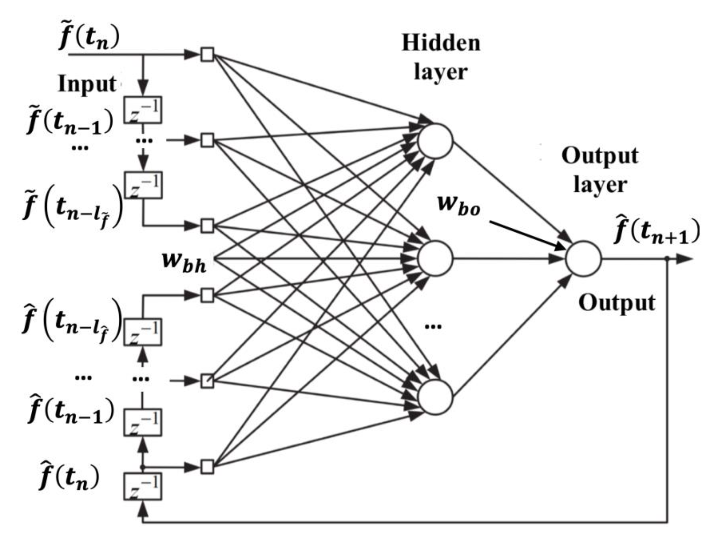
After the wavelet filtering, the signal f ˜ is approximated by the neural NARX network [4,25,27,28]. The architecture of the recurrent NARX PA network [28] is illustrated in Figure 2.
According to the NARX PA network architecture, the network input is f ˜ ( t n ) , and the network output is f ^ ( t n + 1 ) , i.e., the network predicts the data by one step ahead.
The vector, sent to the network hidden layer neurons, consists of the following components:
-
current f ˜ ( t n ) and preliminary values f ˜ ( t n 1 ) , , f ˜ ( t n l f ˜ ) ;
-
output values f ^ ( t n ) , f ^ ( t n 1 ) , , f ^ ( t n l f ^ ) .
The analytical representation of the signal model based on NARX PA has the form
f ^ ( t n + 1 ) = F o ( w b o + h = 1 D w h o · F h ( w b h + i = 0 l f ˜ w i h f ˜ ( t n i ) + z = 0 l f ^ w z h f ^ ( t n z ) ) ) ,
where f ˜ ( t n ) и f ^ ( t n ) is the NN input signal and its approximation by the network, respectively; l f ˜ , l f ^ is the number of delay lines; w z h are weight coefficients of the values arriving from NN output to the hidden layer neurons; w i h are weight coefficients of input values arriving to the hidden layer neurons; w b h and w b o are constant terms for the hidden and output layers, respectively; F h and F o are activation functions for the neurons of the hidden and output layers, respectively; w h o are weight coefficients for the values arriving on output layer neurons; D is the number of hidden layer neurons.
It is known that network architecture affects forecast efficiency. NARX model architecture depends on the size of the embedded memory of input ( l f ˜ ), of output ( l f ^ ) and the neuron number in the hidden layer. It is not a trivial task to determine these parameters. The number of the delay lines of input l f ˜ and output l f ^ can be determined by minimizing the network error [28]. The technique to determine these parameters and the obtained results are represented below in this paper.
The Bayesian regularization algorithm is used for network training. This algorithm updates the weights and the shifts leading to the network neurons according to the Levenberg–Marquardt optimization [25]. The Bayesian regularization technique allows one to form a combination of neuron and weight number of the hidden layer in such a way that the network has the highest degree of generalization [28]. The regularization function minimizes the linear combination of squared errors and weight coefficients of the network at the stage of training. That makes it possible to optimize the neuron number of the hidden layer and to avoid the overtraining effect.

2.3. Scheme of Method Realization

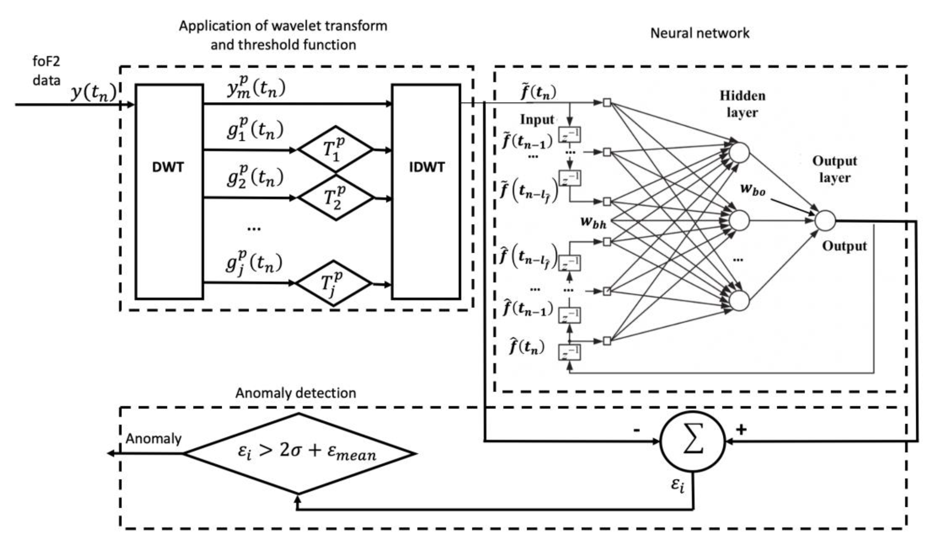
The scheme of method realization is illustrated in Figure 3. Disorder in the system evidently indicates an anomaly in the data. A disorder can be detected based on the analysis of the vector of neural network summary errors estimated in the time window of the length = 2 l + 1
ε i = i = i l i + l | f ^ ( i ) f ˜ ( i ) | .
In this case, we can consider that there is an anomaly in the data if
ε i > 2 σ + ε m e a n ,
where σ is the standard deviation of network summary errors, it is estimated during the periods without anomalies; ε m e a n is the average of network summary errors during the periods without anomalies.

3. Results of Method Application for Ionospheric Data

In the paper, we used the ionospheric layer F2 critical frequency (foF2) data for the period 1969–2015. The data were recorded at IKIR FEB RAS (Paratunka site, Kamchatskiy kray, Russia) from 1968 up to the present time. According to the suggested method, the input and reference values of NN were obtained after the wavelet filtering procedure. In the operations of wavelet filtering, we used orthonormal third-order Daubechies [21], which were determined by minimizing foF2 data approximation errors [60]. To evaluate the method, NN were also trained using the foF2 initial data without wavelet filtering.
When forming training and control NN samples, we took into account the dependence of foF2 data time variation on the season and solar activity level. Thus, NN were constructed for different seasons and different levels of solar activity separately. Two periods of solar activity were considered, the period of high solar activity and the period of low solar activity (the level of solar activity was estimated by mean monthly values of radio emission at the wavelength of f10.7 [61]). To obtain NARX models describing foF2 data regular time variation, data for the periods of calm ionosphere were used in the training process. For each NN, training samples contained one vector of the length from 2000 to 4000 counts. We constructed 24 networks.
When constructing NN, input and output delay lines l f ˜ = l f ^ = 2 , l f ˜ = l f ^ = 3 , l f ˜ = l f ^ = 5 were used. The parameters l f ˜ and l f ^ were determined according to the investigation results of [24]. In the paper [24], an autocorrelation function (ACF) and partial autocorrelation function (PACF) were studied to determine the order of ARIMA models of the foF2 series. It was shown [24] that after wavelet filtering and obtaining the first differences, AR models of foF2 series had the orders 2 and 3 depending on the season and solar activity level. However, we should note that in the general case, the question of the determination of l f ˜ and l f ^ is important and requires additional study. As was shown in the paper [28], the NARX model quality significantly depends on the size of input and output embedded memory.
The selection of NN inner architecture was based on NN error estimates. The standard deviations of errors (STD) for the networks were determined as
STD = 1 N 1 i = 1 N ( e i e ¯ ) 2 ,
where e ¯ = 1 N i = 1 N e i , e i = f ^ 0 ( i ) f 0 ˜ ( i ) .
As an example, Table 1 shows NN error estimates for wintertime depending on the neuron number of the hidden layer. An analysis of Table 1 shows that the STD error decreased when the number of neurons was 20 in the hidden layer. Then, the network error remained unchanged. Based on these results, we determined the wintertime network architecture with the number of neurons of the hidden layer equal to 20. Making similar investigations, we determined the number of neurons of the hidden layer were also equal to 20 for the summertime.
Table 2 shows the STD errors of NN for different delay lines. An analysis of the results shows that the number of NN approximations increased insignificantly as the number of delay lines grew for the NN trained without wavelet filtering. The application of wavelet filtering made it possible to increase significantly the NN approximation quality especially during low solar activity. That confirmed the efficiency of the proposed method.
The results of NN quality estimates, based on the control set data during the periods without anomalies, are illustrated in Table 3. The analysis shows significant improvement of NN approximation quality when using the wavelet filtering procedure. The application of wavelet filtering made it possible to decrease significantly the average error ( ε m e a n ) and STD ( σ ) for different delay lines. We should also note that the application of wavelet filtering allowed us to use the low number of input and output delay lines when the network performance quality was good.
The test for the adequacy of the obtained NARX models was based on the Ljung-Box test [62]:
Q = M ( M + 2 ) s = 1 L ρ s 2 M s ,
where M is the observations number, ρ s is the autocorrelation of the s-th order, and L is the number of lags under the check. If Q > χ 1 α ,   L 2 , where χ 1 α ,   L 2 is the quantile of chi-square distribution with L degrees of freedom, then the presence of autocorrelation of the L-th order in the time series is admitted.
The results of the Ljung-Box test are presented in Table 4. The analysis of the results shows that for the networks constructed without wavelet filtering, Ljung-Box test values exceeded significantly the corresponding critical value χ 1 α ,   L 2 . That indicates the correlation of network errors and, as a sequence, the not-quite-good-enough quality of foF2 data approximation. We should note that the error correlation grew significantly for large lags L that were evidently associated with the presence of long time dependencies (foF2 diurnal variation) in foF2 data. As was mentioned in the paper [28], in the systems with large time dependencies for the training algorithms based on gradient, information on step gradient m in the past vanished at large m (the problem of vanishing gradients). Thus, the application of RNN faces problems when modeling data with long time dependencies, especially when forecasting nonlinear nonstationary signals [28]. It was also shown in the paper [25] that the problem of vanishing gradients made the investigation of long-term dependencies in training algorithms, based on gradient, difficult and in some cases almost impossible. When the delay lines grew, the data approximation quality increased (Table 4). However, the adequacy was confirmed only for NARX models obtained with wavelet filtering. For the network delay lines l f ˜ = l f ^ = 3 ,   l f ˜ = l f ^ = 5 , according to the Ljung-Box test, network errors were uncorrelated. That confirms their adequacy to foF2 data and shows the efficiency of the suggested method.
Figure 4 shows the results of NN performance during a moderate magnetic storm on 16–17 July 2017. A red dashed line in Figure 4 indicates the time of the magnetic storm beginning. To analyze the geomagnetic activity index, DST index values are illustrated in Figure 4e [63]. During the strongest geomagnetic disturbances on 16 July 2017, the DST index reached the minimum of −72 nT (Figure 4e). An analysis of foF2 data (Figure 4a) shows insignificant changes in fluctuation amplitude during the magnetic storm that was determined by ionospheric disturbance occurrences. Median value data (dashed lines in Figure 4a) also confirmed the presence of an anomaly in the ionosphere during the magnetic storm. The processing results (Figure 4b–d,f–h) illustrated a significant increase in NN errors during the strongest geomagnetic disturbances that indicated anomalous changes in the data. The comparison of the results of the NN trained on the initial data (Figure 4b–d) with the results of the NN obtained after wavelet filtering (Figure 4f–h) confirmed the significant improvement of NN quality when using wavelet filtering. Errors of the NN trained after the wavelet filtering procedure were close to zero. In the error vector of the NN trained on the initial data, an oscillation process was observed which was likely to be associated with foF2 diurnal variation. The result confirms the assumption mentioned above that the application of RNN faced problems when modeling the data with long time dependencies (problem of vanishing gradients). The result also confirms the efficiency of the suggested wavelet filtering procedure to improve the NARX performance quality when modeling nonstationary and noisy data.
Comparing the results of NN with a different number of delay lines, we have learned that for the delay lines l f ˜ = l f ^ = 5 (Figure 4h), anomalous changes were detected on a longer interval that agreed well with the obtained median values of foF2 (dashed line in Figure 4a). A comparison of the NARX results with the median method shows a higher efficiency of the NN. Due to the significant nonstationarity of foF2 data time variation during the magnetic storm, there were errors in median values during the period after the storm on 18 July 2017. There were no errors in the NN model.
Figure 5 shows the results of data processing during a weak magnetic storm on 5–6 August 2019. The red vertical line indicates the magnetic storm beginning (Figure 5). Results in Figure 5 are similar to those illustrated above for the event on 16–17 July 2017. The estimated median values (Figure 5a) show long changes in foF2 data time variation during the magnetic storm. An analysis of NN errors also shows their increase during the event that indicates anomaly occurrence in the ionosphere. The comparison of the results of NN performance without wavelet filtering (Figure 5b–d) and with wavelet filtering (Figure 5f–h) shows a significant decrease in NN errors based on the suggested approach. That is similar to the results of the event on 16–17 July 2017. The NN with the delay lines l f ˜ = l f ^ = 5 (Figure 5h) shows the best results. It has the least errors and the anomalous period in ionospheric data is clearly detectable.
Table 5 shows quantitative estimates of the NN performance during the events described above. The estimates were carried out separately during calm and disturbed periods. An analysis of the results from Table 5 shows that wavelet filtering allows one to decrease significantly the average values of network errors and their STD during calm periods. A decrease in the NN error level by more than 3 times is observed after the wavelet filtering procedure. During the anomalous period, the STD of the network trained after the wavelet filtering may increase by 17 times. That makes it possible to detect anomalous changes in the ionosphere accurately. We should also note that as the number of delay lines increase, the quality of anomaly detection by this network improves. The results confirm the efficiency of the suggested method.

4. Conclusions

The application of the method showed its efficiency in the problem of ionospheric data modeling and analysis. The suggested procedure of wavelet filtering allows us to improve the NARX neural network performance quality and gives the possibility to obtain an adequate model for noisy and nonstationary data.
As was mentioned in the papers [25,28], data modeling based on NARX has some difficulties associated with the presence of long time dependences caused by the “vanishing gradient”. It was shown on the example of ionospheric data that the wavelet filtering procedure makes it possible to solve this problem if there is a long period. The Ljung-Box test confirmed the adequacy of the obtained neural network models.
On the example of the magnetic storms that occurred on 16–17 July 2017 and on 5–6 August 2019, we confirmed the possibility to apply the method for the detection of ionospheric anomalies based on foF2 data during magnetospheric disturbances. A comparison of the NARX network with the median method, traditionally used for ionospheric data analysis, showed the NN efficiency. The ionospheric data time variation change during the magnetic storms under analysis entailed error occurrences in the estimates of median values, which were absent in the NN model. The method can be used to monitor the ionosphere state during space weather forecasting.
We plan to continue the investigation in this direction involving ionospheric data from other regions. We also plan to apply the developed method for a more detailed study of ionospheric parameters during increased solar activity and magnetic storms.

Author Contributions

Conceptualization, O.M.; methodology, O.M. and Y.P.; software, Y.P.; validation, Y.P. and N.Z.; formal analysis, O.M. and Y.S.; investigation, O.M. and Y.P.; resources, N.Z. and Y.S.; data curation, Y.P.; writing—original draft preparation, Y.P.; writing—review and editing, O.M.; project administration, O.M.; funding acquisition, Y.S. All authors have read and agreed to the published version of the manuscript.

Funding

This work was supported by the Ministry of Science and Higher Education of the Russian Federation by the Agreement № 075-15-2022-291 on the provision of a grant in the form of subsidies from the federal budget for the implementation of state support for the establishment and development of the world-class scientific center «Pavlov center «Integrative physiology for medicine, high-tech healthcare, and stress-resilience technologies».

Institutional Review Board Statement

Not applicable.

Informed Consent Statement

Not applicable.

Data Availability Statement

Not applicable.

Acknowledgments

The work was carried out according to the Subject AAAA-A21-121011290003-0 “Physical processes in the system of near space and geospheres under solar and lithospheric influences” IKIR FEB RAS. The work was realized by the means of the Common Use Center “North-Eastern Heliogeophysical Center” CKP_558279, USU 351757. The authors are grateful to the World Data Center for Geomagnetism, Kyoto (http://wdc.kugi.kyoto-u.ac.jp/dstae/index.html (accessed on 20 June 2022)).

Conflicts of Interest

The authors declare no conflict of interest.

Appendix A

NAS algorithm [54]:
(1) signal X is decomposed into wavelet packets
W j 0 : W j 0 = i = 0 I W j i p i , { Ψ j i p i ( 2 j i t m ) } m   is the basis of the space W j i p i ;
(2) based on the estimate of normalized energies, we determine the tree branches corresponding to signal structural components: basis B j i p i of the space W j i p i is the basis
B j i p i = { { Ψ j i p i ( 2 j i t m ) } m ,   i f   m I p i | X , Ψ j i , m p i | 2 m I 2 p i | X , Ψ j i + 1 , m 2 p i | 2 + m I 2 p i + 1 | X , Ψ j i + 1 , m 2 p i + 1 | 2 { Ψ j i + 1 2 p i } m   { Ψ j i + 1 2 p i + 1 } m ,   i f m I p i | X , Ψ j i , m p i | 2 < m I 2 p i | X , Ψ j i + 1 , m 2 p i | 2 + m I 2 p i + 1 | X , Ψ j i + 1 , m 2 p i + 1 | 2
where the index set I l ,   l = p i ,   2 p i ,   2 p i + 1 is determined as follows: index m I l , if | X , Ψ j i ,   m l | T j i , threshold T j i = K σ j i l ,   σ j i l = 1 L m = 1 L ( X , Ψ j i ,   m l X , Ψ j i , m l ¯ ) 2 , where the coefficient of the threshold K is determined by estimating a posterior risk, X , Ψ j i , m l ¯ is the average of the set { | X , Ψ j i , m l | } 0 m < L , L is the element number.

References

  1. Alperovich, L.; Eppelbaum, L.; Zheludev, V.; Dumoulin, J.; Soldovieri, F.; Proto, M.; Bavusi, M.; Loperte, A. A New Combined Wavelet Methodology: Implementation to GPR and ERT Data Obtained in the Montagnole Experiment. J. Geophys. Eng. 2013, 10, 025017. [Google Scholar] [CrossRef]
  2. Bailey, R.L.; Leonhardt, R. Automated Detection of Geomagnetic Storms with Heightened Risk of GIC. Earth Planets Space 2016, 68, 99. [Google Scholar] [CrossRef] [Green Version]
  3. Tang, R.; Zeng, F.; Chen, Z.; Wang, J.-S.; Huang, C.-M.; Wu, Z. The Comparison of Predicting Storm-Time Ionospheric TEC by Three Methods: ARIMA, LSTM, and Seq2Seq. Atmosphere 2020, 11, 316. [Google Scholar] [CrossRef] [Green Version]
  4. Boussaada, Z.; Curea, O.; Remaci, A.; Camblong, H.; Mrabet Bellaaj, N. A Nonlinear Autoregressive Exogenous (NARX) Neural Network Model for the Prediction of the Daily Direct Solar Radiation. Energies 2018, 11, 620. [Google Scholar] [CrossRef] [Green Version]
  5. Chierici, F.; Embriaco, D.; Pignagnoli, L. A New Real-Time Tsunami Detection Algorithm: Tsunami detection algorithm. J. Geophys. Res. Oceans 2017, 122, 636–652. [Google Scholar] [CrossRef]
  6. Kim, S.-K.; Lee, E.; Park, J.; Shin, S. Feasibility Analysis of GNSS-Reflectometry for Monitoring Coastal Hazards. Remote Sens. 2021, 13, 976. [Google Scholar] [CrossRef]
  7. Perol, T.; Gharbi, M.; Denolle, M. Convolutional Neural Network for Earthquake Detection and Location. Sci. Adv. 2018, 4, e1700578. [Google Scholar] [CrossRef] [PubMed] [Green Version]
  8. Amigó, J.M.; Small, M. Mathematical Methods in Medicine: Neuroscience, Cardiology and Pathology. Philos. Trans. R. Soc. A 2017, 375, 20170016. [Google Scholar] [CrossRef] [PubMed] [Green Version]
  9. Marple, S.L. Digital Spectral Analysis: With Applications; Prentice-Hall signal processing series; Prentice-Hall: Englewood Cliffs, NJ, USA, 1987; ISBN 978-0-13-214149-9. [Google Scholar]
  10. Box, G.E.P.; Jenkins, G.M. Time Series Analysis: Forecasting and Control, Revised Edition; Holden-Day series in time series analysis and digital processing; Holden-Day: San Francisco, CA, USA, 1976; ISBN 978-0-8162-1104-3. [Google Scholar]
  11. Liu, J.; Kumar, S.; Palomar, D.P. Parameter Estimation of Heavy-Tailed AR Model With Missing Data Via Stochastic EM. IEEE Trans. Signal Process. 2019, 67, 2159–2172. [Google Scholar] [CrossRef] [Green Version]
  12. Robbins, H.; Monro, S. A Stochastic Approximation Method. Ann. Math. Stat. 1951, 22, 400–407. [Google Scholar] [CrossRef]
  13. Estévez, J.; Bellido-Jiménez, J.A.; Liu, X.; García-Marín, A.P. Monthly Precipitation Forecasts Using Wavelet Neural Networks Models in a Semiarid Environment. Water 2020, 12, 1909. [Google Scholar] [CrossRef]
  14. Pavlicko, M.; Vojteková, M.; Blažeková, O. Forecasting of Electrical Energy Consumption in Slovakia. Mathematics 2022, 10, 577. [Google Scholar] [CrossRef]
  15. Gocheva-Ilieva, S.; Yordanova, A.; Kulina, H. Predicting the 305-Day Milk Yield of Holstein-Friesian Cows Depending on the Conformation Traits and Farm Using Simplified Selective Ensembles. Mathematics 2022, 10, 1254. [Google Scholar] [CrossRef]
  16. Li, S.; Wang, Q. India’s Dependence on Foreign Oil Will Exceed 90% around 2025—The Forecasting Results Based on Two Hybridized NMGM-ARIMA and NMGM-BP Models. J. Clean. Prod. 2019, 232, 137–153. [Google Scholar] [CrossRef]
  17. Wu, X.; Zhou, J.; Yu, H.; Liu, D.; Xie, K.; Chen, Y.; Hu, J.; Sun, H.; Xing, F. The Development of a Hybrid Wavelet-ARIMA-LSTM Model for Precipitation Amounts and Drought Analysis. Atmosphere 2021, 12, 74. [Google Scholar] [CrossRef]
  18. Mbatha, N.; Bencherif, H. Time Series Analysis and Forecasting Using a Novel Hybrid LSTM Data-Driven Model Based on Empirical Wavelet Transform Applied to Total Column of Ozone at Buenos Aires, Argentina (1966–2017). Atmosphere 2020, 11, 457. [Google Scholar] [CrossRef]
  19. Mehdizadeh, S.; Fathian, F.; Adamowski, J.F. Hybrid Artificial Intelligence-Time Series Models for Monthly Streamflow Modeling. Appl. Soft Comput. 2019, 80, 873–887. [Google Scholar] [CrossRef]
  20. Mallat, S.G. A Wavelet Tour of Signal Processing; Academic Press: San Diego, CA, USA, 1999; ISBN 978-0-12-466606-1. [Google Scholar]
  21. Daubechies, I. Ten Lectures on Wavelets; Society for Industrial and Applied Mathematics: Philadelphia, PA, USA, 1992; ISBN 978-0-89871-274-2. [Google Scholar]
  22. Chui, C.K. An Introduction to Wavelets; Wavelet analysis and its applications; Academic Press: Boston, MA, USA, 1992; ISBN 978-0-12-174584-4. [Google Scholar]
  23. Mandrikova, O.; Polozov, Y.; Fetisova, N.; Zalyaev, T. Analysis of the Dynamics of Ionospheric Parameters during Periods of Increased Solar Activity and Magnetic Storms. J. Atmos. Sol.-Terr. Phys. 2018, 181, 116–126. [Google Scholar] [CrossRef]
  24. Mandrikova, O.; Fetisova, N.; Polozov, Y. Hybrid Model for Time Series of Complex Structure with ARIMA Components. Mathematics 2021, 9, 1122. [Google Scholar] [CrossRef]
  25. Haykin, S.S. Neural Networks: A Comprehensive Foundation, 2nd ed.; Prentice Hall: Upper Saddle River, NJ, USA, 1999; ISBN 978-0-13-273350-2. [Google Scholar]
  26. Singh, J.; Barabanov, N. Stability of Discrete Time Recurrent Neural Networks and Nonlinear Optimization Problems. Neural Netw. 2016, 74, 58–72. [Google Scholar] [CrossRef]
  27. Ma, Q.; Liu, S.; Fan, X.; Chai, C.; Wang, Y.; Yang, K. A Time Series Prediction Model of Foundation Pit Deformation Based on Empirical Wavelet Transform and NARX Network. Mathematics 2020, 8, 1535. [Google Scholar] [CrossRef]
  28. Diaconescu, E. The use of NARX neural networks to predict chaotic time series. WSEAS Trans. Comp. Res. 2008, 3, 182–191. [Google Scholar]
  29. Lin, T.; Horne, B.G.; Tino, P.; Giles, C.L. Learning Long-Term Dependencies in NARX Recurrent Neural Networks. IEEE Trans. Neural Netw. 1996, 7, 1329–1338. [Google Scholar] [CrossRef] [PubMed] [Green Version]
  30. Gao, Y.; Er, M.J. NARMAX Time Series Model Prediction: Feedforward and Recurrent Fuzzy Neural Network Approaches. Fuzzy Sets Syst. 2005, 150, 331–350. [Google Scholar] [CrossRef]
  31. Tsungnan, L.; Giles, C.L.; Horne, B.G.; Kung, S.Y. A Delay Damage Model Selection Algorithm for NARX Neural Networks. IEEE Trans. Signal Process. 1997, 45, 2719–2730. [Google Scholar] [CrossRef] [Green Version]
  32. Dorffner, G. Neural Networks for Time Series Processing. Neural Netw. World 1996, 6, 447–468. [Google Scholar]
  33. Mandic, D.P.; Chambers, J.A. Recurrent Neural Networks for Prediction: Learning Algorithms, Architectures, and Stability; Wiley series in adaptive and learning systems for signal processing, communications, and control; John Wiley: Chichester, UK; New York, NY, USA, 2001; ISBN 978-0-471-49517-8. [Google Scholar]
  34. Mandrikova, O.; Mandrikova, B. Hybrid Method for Detecting Anomalies in Cosmic ray Variations Using Neural Networks Autoencoder. Symmetry 2022, 14, 744. [Google Scholar] [CrossRef]
  35. Mandrikova, O.; Mandrikova, B. Method of Wavelet-Decomposition to Research Cosmic Ray Variations: Application in Space Weather. Symmetry 2021, 13, 2313. [Google Scholar] [CrossRef]
  36. Phan, T.-T.-H.; Nguyen, X.H. Combining Statistical Machine Learning Models with ARIMA for Water Level Forecasting: The Case of the Red River. Adv. Water Resour. 2020, 142, 103656. [Google Scholar] [CrossRef]
  37. Bengio, Y.; Simard, P.; Frasconi, P. Learning Long-Term Dependencies with Gradient Descent Is Difficult. IEEE Trans. Neural Netw. 1994, 5, 157–166. [Google Scholar] [CrossRef]
  38. Schaefer, A.M.; Udluft, S.; Zimmermann, H.-G. Learning Long-Term Dependencies with Recurrent Neural Networks. Neurocomputing 2008, 71, 2481–2488. [Google Scholar] [CrossRef]
  39. Glüge, S.; Böck, R.; Palm, G.; Wendemuth, A. Learning Long-Term Dependencies in Segmented-Memory Recurrent Neural Networks with Backpropagation of Error. Neurocomputing 2014, 141, 54–64. [Google Scholar] [CrossRef]
  40. Pascanu, R.; Mikolov, T.; Bengio, Y. On the difficulty of training Recurrent Neural Networks. In Proceedings of the 30th International Conference on Machine Learning, Atlanta, GA, USA, 17–19 June 2013. [Google Scholar]
  41. Zhang, J.; Lin, Y.; Song, Z.; Dhillon, I.S. Learning Long Term Dependencies via Fourier Recurrent Units. Int. Conf. Mach. Learn. 2018, 80, 5815–5823. [Google Scholar] [CrossRef]
  42. Yue, B.; Fu, J.; Liang, J. Residual Recurrent Neural Networks for Learning Sequential Representations. Information 2018, 9, 56. [Google Scholar] [CrossRef] [Green Version]
  43. Gers, F.A.; Schmidhuber, J.; Cummins, F. Learning to Forget: Continual Prediction with LSTM. Neural Comput. 2000, 12, 2451–2471. [Google Scholar] [CrossRef]
  44. Hochreiter, S.; Schmidhuber, J. Long Short-Term Memory. Neural Comput. 1997, 9, 1735–1780. [Google Scholar] [CrossRef]
  45. Kühnert, C.; Gonuguntla, N.M.; Krieg, H.; Nowak, D.; Thomas, J.A. Application of LSTM Networks for Water Demand Prediction in Optimal Pump Control. Water 2021, 13, 644. [Google Scholar] [CrossRef]
  46. Jiao, F.; Huang, L.; Song, R.; Huang, H. An Improved STL-LSTM Model for Daily Bus Passenger Flow Prediction during the COVID-19 Pandemic. Sensors 2021, 21, 5950. [Google Scholar] [CrossRef]
  47. Li, P.; Zhang, J.; Krebs, P. Prediction of Flow Based on a CNN-LSTM Combined Deep Learning Approach. Water 2022, 14, 993. [Google Scholar] [CrossRef]
  48. Noh, S.-H. Analysis of Gradient Vanishing of RNNs and Performance Comparison. Information 2021, 12, 442. [Google Scholar] [CrossRef]
  49. Greff, K.; Srivastava, R.K.; Koutnik, J.; Steunebrink, B.R.; Schmidhuber, J. LSTM: A Search Space Odyssey. IEEE Trans. Neural Netw. Learn. Syst. 2017, 28, 2222–2232. [Google Scholar] [CrossRef] [PubMed] [Green Version]
  50. Gers, F. Long Short-Term Memory in Recurrent Neural Networks; EPFL: Lausanne, Switzerland, 2001. [Google Scholar] [CrossRef]
  51. Danilov, A.D. Ionospheric F-Region Response to Geomagnetic Disturbances. Adv. Space Res. 2013, 52, 343–366. [Google Scholar] [CrossRef]
  52. Tebabal, A.; Radicella, S.M.; Nigussie, M.; Damtie, B.; Nava, B.; Yizengaw, E. Local TEC Modelling and Forecasting Using Neural Networks. J. Atmos. Sol.-Terr. Phys. 2018, 172, 143–151. [Google Scholar] [CrossRef]
  53. Dmitriev, A.V.; Suvorova, A.V.; Klimenko, M.V.; Klimenko, V.V.; Ratovsky, K.G.; Rakhmatulin, R.A.; Parkhomov, V.A. Predictable and Unpredictable Ionospheric Disturbances during St. Patrick’s Day Magnetic Storms of 2013 and 2015 and on 8–9 March 2008. J. Geophys. Res. Space Phys. 2017, 122, 2398–2423. [Google Scholar] [CrossRef]
  54. Mandrikova, O.; Mandrikova, B.; Rodomanskay, A. Method of Constructing a Nonlinear Approximating Scheme of a Complex Signal: Application Pattern Recognition. Mathematics 2021, 9, 737. [Google Scholar] [CrossRef]
  55. Rudin, W. Functional Analysis. In International Series in Pure and Applied Mathematics, 2nd ed.; McGraw-Hill: New York, NY, USA, 1991; ISBN 978-0-07-054236-5. [Google Scholar]
  56. Korostelev, A.P.; Korosteleva, O. Mathematical Statistics: Asymptotic Minimax Theory; Graduate studies in mathematics; American Mathematical Society: Providence, RI, USA, 2011; ISBN 978-0-8218-5283-5. [Google Scholar]
  57. Berger, J.O. Statistical Decision Theory and Bayesian Analysis, 2nd ed.; Springer series in statistics; Springer: New York, NY, USA, 1993; ISBN 978-0-387-96098-2. [Google Scholar]
  58. Zhang, X.-M. Schur-Convex Functions and Isoperimetric Inequalities. Proc. Am. Math. Soc. 1998, 126, 461–470. [Google Scholar] [CrossRef] [Green Version]
  59. Priestley, M.B.; Priestley, M.B. Spectral Analysis and Time Series; Probability and mathematical statistics; Repr.; Elsevier: Amsterdam, The Netherlands; Heidelberg, Germany, 2004; ISBN 978-0-12-564922-3. [Google Scholar]
  60. Mandrikova, O.; Polozov, Y.; Geppener, V. Method of Ionospheric Data Analysis Based on a Combination of Wavelet Transform and Neural Networks. Procedia Eng. 2017, 201, 756–766. [Google Scholar] [CrossRef]
  61. Tapping, K.F. The 10.7 Cm Solar Radio Flux (F10.7): F10.7. Space Weather. 2013, 11, 394–406. [Google Scholar] [CrossRef]
  62. Ljung, G.M.; Box, G.E. On a measure of lack of fit in time series models. Biometrika 1978, 65, 297–303. [Google Scholar] [CrossRef]
  63. Sugiura, M. Hourly values of equatorial Dst for the IGY. Ann. Int. Geophys. Year 1964, 35, 7–45. [Google Scholar]
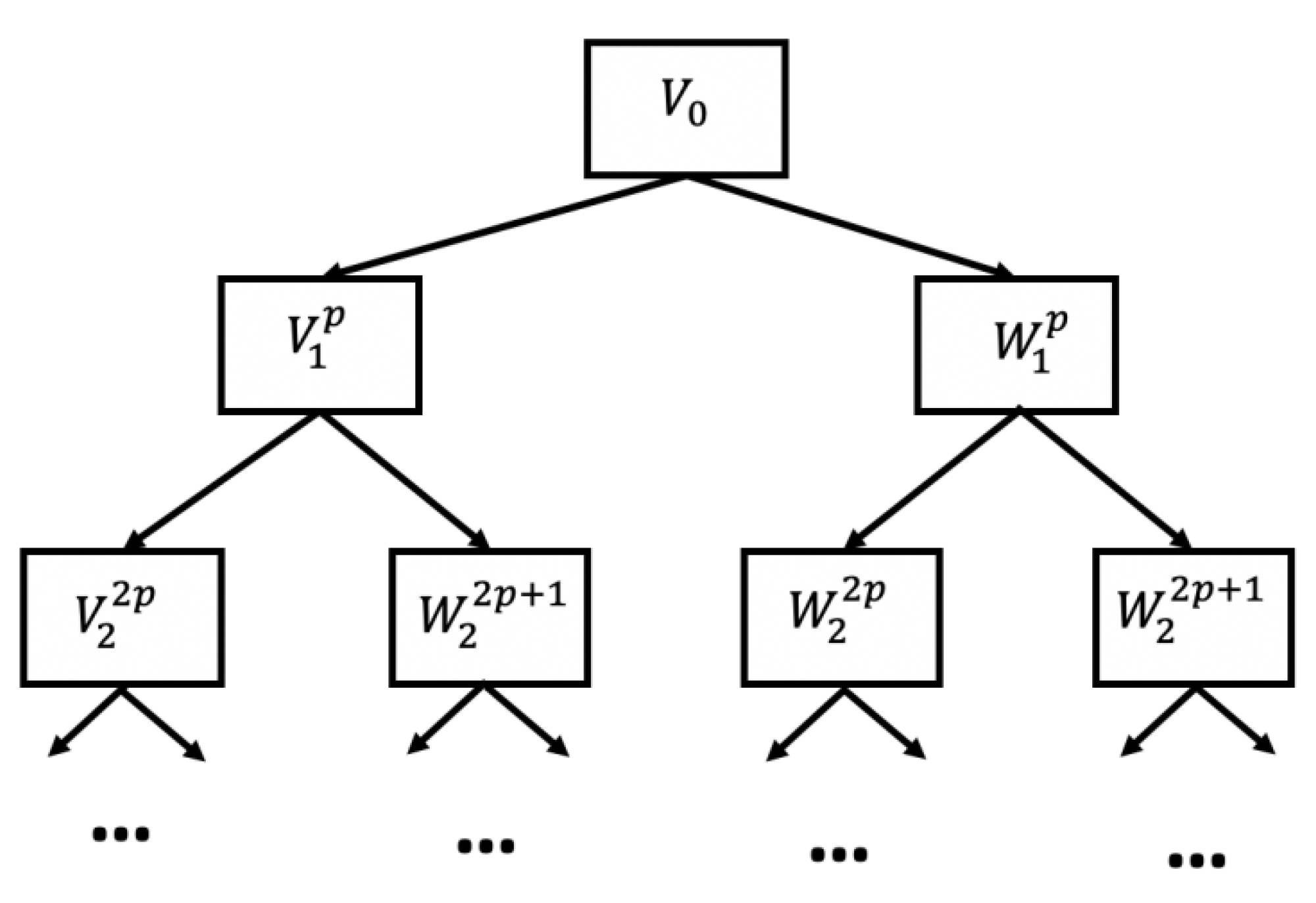
Figure 1. Wavelet packet tree.
Mathematics 10 04345 g001
Figure 2. Architecture of the recurrent NARX PA network.
Mathematics 10 04345 g002
Figure 3. Scheme of method realization.
Mathematics 10 04345 g003
Figure 4. Results of data processing for the period 14–19 July 2017. (a) foF2 initial data (black) and foF2 median (green); (bd) NN errors with delays 2, 3, and 5, respectively, obtained without wavelet filtering; (e) DST; (fh) errors with delays 2, 3, and 5, respectively, obtained with wavelet filtering. Red dashed line is the magnetic storm beginning.
Mathematics 10 04345 g004
Figure 5. Results of data processing for the period 3–8 August 2019. (a) foF2 initial data (black) and foF2 median (green); (bd) NN errors with delays 2, 3, and 5, respectively, obtained without wavelet filtering; (e) DST; (fh) errors with delays 2, 3, and 5, respectively, obtained with wavelet filtering. Red dashed line is the magnetic storm beginning.
Mathematics 10 04345 g005
Table 1. Construction of network architecture for the data during winter season and high solar activity.
Neuron Number481216202428
STD0.540.480.420.420.400.400.41
Table 2. Standard deviations of neural network errors.
SeasonDelay 2Delay 2
Wavelet Filtering
Delay 3Delay 3
Wavelet Filtering
Delay 5Delay 5
Wavelet Filtering
Winter (low solar activity)0.710.490.690.50.690.49
Summer (low solar activity)0.60.330.540.320.460.27
Winter (high solar activity)1.30.871.310.851.30.87
Summer (high solar activity)0.540.50.520.510.490.49
Table 3. Results of NN performance (summer and winter, low solar activity).
Delay Lines
l f ˜ = l f ^
Season ε m e a n y
without Wavelet Filtering
σ y
without Wavelet Filtering
ε m e a n f ˜
with Wavelet Filtering
σ f ˜
with Wavelet Filtering
2Sum1.30.60.480.33
3Sum1.420.540.470.32
5Sum1.270.460.460.27
2Win1.390.710.650.49
3Win1.240.690.670.50
5Win1.210.690.640.49
Table 4. Ljung-Box test values (summer, low solar activity).
Delay Lines
l x = l y
Lag Number L Q y without
Wavelet Filtering
Q f ˜
with Wavelet Filtering
χ 1 α ,     L 2
210.041.473.84
2430.416.39.48
2869.128.115.5
21212841.721
310.020.043.84
340.91.99.48
3812.69.615.5
31264.918.221
510.50.053.84
541.43.89.48
5815.615.215.5
51244.619.921
Table 5. Results of NN performance.
Delay Lines
l f ˜ = l f ^
Year ε m e a n y
without Wavelet Filtering
σ y
without Wavelet Filtering
ε m e a n f ˜
with Wavelet Filtering
σ f ˜
with Wavelet Filtering
calm period
220171.020.630.390.27
320171.050.570.370.24
520170.980.530.240.15
220191.170.610.420.29
320191.420.640.310.24
520191.310.580.330.12
anomaly period
220171.861.191.811.4
320171.831.111.61.64
520171.650.942.581.7
220191.831.411.681.2
320192.021.062.181.96
520192.160.972.882.05
Publisher’s Note: MDPI stays neutral with regard to jurisdictional claims in published maps and institutional affiliations.