Fuzziness, Indeterminacy and Soft Sets: Frontiers and Perspectives

Abstract

The present paper comes across the main steps that were laid from Zadeh’s fuzziness and Atanassov’s intuitionistic fuzzy sets to Smarandache’s indeterminacy and to Molodstov’s soft sets. Two hybrid methods for assessment and decision making, respectively, under fuzzy conditions are also presented using suitable examples that use soft sets and real intervals as tools. The decision making method improves on an earlier method of Maji et al. Further, it is described how the concept of topological space, the most general category of mathematical spaces, can be extended to fuzzy structures and how to generalize the fundamental mathematical concepts of limit, continuity compactness and Hausdorff space within such kinds of structures. In particular, fuzzy and soft topological spaces are defined and examples are given to illustrate these generalizations.

1. Introduction

1.1. Multi-Valued LOGICS

The development of human science and civilization owes a lot to Aristotle’s (384–322 BC) bivalent logic (BL), which was at the center of human reasoning for more than two thousand years. BL is based on the “Principle of the Excluded Middle”, according to which each proposition is either true or false.

Opposite views also appeared early in human history, however, supporting the existence of a third area between true and false, where these two notions can exist together; e.g., by Buddha Siddhartha Gautama (India, around 500 BC), by Plato (427–377 BC), and more recently by the philosophers Hegel, Marx, Engels, etc. Integrated propositions of multi-valued logics appeared, however, only during the early 1900s by Lukasiewicz, Tarski, and others. According to the “Principle of Valence”, formulated by Lukasiewicz, propositions are not only either true or false, but they can have an intermediate truth-value.

1.2. Literature Review

Zadeh introduced, in 1965, the concept of fuzzy set (FS) [1] and with the help of this developed the infinite in the unit interval [0, 1] fuzzy logic [2] with the purpose of dealing with partial truths. FL, where truth values are modelled by numbers in the unit interval, satisfies the Lukasiewicz’s “Principle of Valence”. It was only in a second moment that FS theory and FL were used to embrace uncertainty modelling [3,4]. This happened when membership functions were reinterpreted as possibility distributions. Possibility theory is an uncertainty theory devoted to the handling of incomplete information [5]. Zadeh articulated the relationship between possibility and probability, noticing that what is probable must preliminarily be possible [3].

The uncertainty that exists in everyday life and science is connected to inadequate information about the corresponding case. A reduction, therefore, of the existing uncertainty (via new evidence) means the addition of an equal piece of information. This is why the methods of measuring information (Hartley’s formula, Shannon’s entropy, etc.) are also used for measuring uncertainty and vice versa; e.g., see ([6], Chapter 5).

Probability theory used to be, for a long period, the unique way to deal with problems connected to uncertainty. Probability, however, is suitable only for tackling cases of uncertainty that are due to randomness [7]. However, randomness characterizes events with known outcomes that cannot be predicted in advance, e.g., games of chance. Starting from Zadeh’s FS, however, various generalizations of FSs and other related theories have been proposed enabling, among others, a more effective management of all types of existing uncertainty. These generalizations and theories include type-n FS, n ≥ 2 [8], interval-valued FS [9], intuitionistic FS (IFS) [10], hesitant FS [11], Pythagorean FS [12], neutrosophic set [13], complex FS [14], grey system [15], rough set [16], soft set (SS) [17], picture FS [18], etc. A brief description of all the previous generalizations and theories, the catalogue of which does not end here, can be found in [19].

Fuzzy mathematics have found many and important practical applications (e.g., see [6,20,21,22,23,24], etc.), but also have interesting connections with branches of pure mathematics, such as Algebra, Geometry, Topology, etc. (e.g., see [25,26], etc.).

1.3. Organization of the Paper

The paper at hand reviews the process that was laid from Zadeh’s fuzziness and Atanassov’s IFS to Smarandache’s indeterminacy and to Molodstov’s soft set. It also presents, using suitable examples, two hybrid methods for assessment and decision making (DM) under fuzzy conditions using SS and real intervals as tools, and describes how one can extend in a natural way the fundamental notion of topological space (TS) to fuzzy structures and can generalize the fundamental mathematical concepts of limit, continuity compactness, etc. within such kinds of structures. More explicitly, Section 2 contains the basics about FSs and FL needed for this work. In Section 3, the concepts of IFS and NS are defined. The concept of SS is presented in Section 4, where basic operations on SSs are also defined. The hybrid assessment and DM methods are developed in Section 5 and the notion of TS is extended to fuzzy structures in Section 6. The last section, Section 7, contains the article’s final conclusion and some suggestions for future research.

2. Fuzzy Sets and Fuzzy Logic

This section contains the basic information about FSs and FL needed for the understanding of the rest of the paper.

2.1. Fuzzy Sets and Systems

Zadeh defined the concept of FS as follows [1]:

Definition 1.

Let U be the universe, then a FS F in U is of the form

$$\mathrm{F}=\left\{\right(\mathrm{x},\mathrm{m}\left(\mathrm{x}\right)):\mathrm{x}\in \mathrm{U}\}$$

(1)

In (1) m: U $\to$ [0, 1] is the membership function of F and m(x) is called the membership degree of x in F. The closer m(x) to 1, the better x satisfies the property of F.

A crisp subset F of U is a FS in U with membership function such that m(x) = 1 if x belongs to F and 0 otherwise.

FSs successfully tackle the uncertainty due to vagueness, which is created when one is unable to distinguish between two properties, such as “a good player” and “a mediocre player”. A serious disadvantage of FSs, however, is that there is not any exact rule for properly defining their membership function. The methods used for this are usually statistical, intuitive or empirical. Moreover, the definition of the membership function is not unique depending on the “signals” that each person receives from the environment. For example, defining the FS of “old people”, one could consider as old all those aged more than 50 years and for another one, all those aged more than 60 years. As a result, the first person will assign membership degree 1 to all people aged between 50 and 60 years, whereas the second will assign membership degrees less than 1. Analogous differences will appear, therefore, to the membership degrees of all the other people. Consequently, the only restriction for the definition of the membership function is that it must be compatible with common sense; otherwise, the resulting FS does not give a creditable description of the corresponding real case. This could happen, for instance, if in the previous example, people aged less than 20 years possessed membership degrees ≥ 0.5.

Definition 2.

The universal FS F_U and the empty FS F_∅ in the universe U are defined as the FSs on U with membership functions m(x) = 1 and m(x) = 0 respectively, for all x in U.

Definition 3.

If K and L are FSs in U with membership functions m_K and m_L respectively, then K is called a fuzzy subset of L if m_K(x) ≤ m_L(x), for all x in U. We write then K $\subseteq$ L. If m_K(x) < m_L(x), for all x in U, then K is said to be a proper fuzzy subset of L and we write K $\subset$ L.

Definition 4.

If K and L are FSs in U with membership functions m_K and m_L respectively, then:

• The union K∪L is said to be the FS in U with membership function m_K∪L(x) = max {m_K(x), m_L (x)}, for each x in U.
• The intersection K∩L is said to be the FS in U with membership function m _K∩L (x) = min {m_K(x), m_L (x)}, for each x in U.
• The complement of K is the FS K* in U with membership function m*(x) = 1 − m(x), for all x in U.

If K and L are crisp subsets of U, then all of the previous definitions reduce to the ordinary definitions for crisp sets.

Zadeh realized that FSs correspond to words (adjectives or adverbs) of the natural language [27]; e.g., the word “clever” corresponds to the FS of clever people, since how clever everyone is, is a matter of degree. A synthesis of FSs related to each other is said to be a fuzzy system, which mimics the way of human reasoning. For example, a fuzzy system can control the function of an air-conditioner, or can send signals for purchasing shares, etc. [21].

2.2. Probabilistic vs. Fuzzy Logic—Bayesian Reasoning

Many of the traditional supporters of the classical BL claimed that, since BL works effectively in science and computing and explains the phenomena of the real world, except perhaps those that happen in the boundaries, there is no reason to introduce the unstable principles of a multi-valued logic. FL, however, aims exactly at clearing the happenings in the boundaries! Look, for example, at Figure 1 [28] representing the FS T of “tall people”. People with a height less than 1.50 m possess a membership degree 0 in T. The membership degrees increase for heights greater than 1.50 m, taking the value 1 for heights as being equal to or greater than 1.80 m. Therefore, the “fuzzy part” of the graph—which is represented, for simplicity, in Figure 1 by the straight line segment AC—but its exact form depends upon the definition of the membership function—lies in the area of the rectangle ABCD formed by the OX axis, its parallel passing through point E and the two perpendicular to the OX lines at points A and B.

BL, on the contrary, considers a boundary (e.g., 1.8 m) above which people are tall and below which they are short. Thus, an individual with a height of 1.805 m is considered to be tall, whereas another with a height of 1.795 m is considered to be short!

In conclusion, FL generalizes and completes the traditional BL fitting better, not only to our everyday life situations, but also to the scientific way of thinking. More details about FL can be found in Section 2 of [28].

E. Jaynes argued that probability theory is a generalization of BL, reducing it in cases where something is either absolutely true or absolutely false [29]. A considerable number of scientists, such as D. Mumford, famous for his contributions to Algebraic Geometry [30], supported his ideas. Nevertheless, as we have already seen in our Introduction, probability, due to its bivalent texture, effectively tackles the uncertainty due to randomness. Therefore, Jaynes’ probabilistic logic is subordinate to FL.

Bayesian Reasoning, however, connects BL and FL [31]. In fact, the Bayes’ rule expressed by Equation (2) below, calculates the conditional probability P(A/B) with the help of P(B/A), of the prior probability P(A) and the posterior probability P(B)

$$\mathrm{P}(\mathrm{A}/\mathrm{B})=\frac{\mathrm{P}(\mathrm{B}/\mathrm{A})\mathrm{P}\left(\mathrm{A}\right)}{\mathrm{P}\left(\mathrm{B}\right)}$$

(2)

The value of P(A) is fixed before the experiment, whereas the value of P(B) is obtained from the experiment’s data. Frequently, however, the value of P(A) is not standard. In such cases, different values of the conditional probability P(A/B) are obtained for all the possible values of P(A). Consequently, Bayes’ rule tackles the existing, due to the imprecision of the value of the prior probability, uncertainty in a way analogous to FL ([32], Section 5).

Bayesian reasoning is very important in everyday life situations and for the whole science too. Recent researches have shown that most of the mechanisms under which the human brain works are Bayesian [33]. Thus, Bayesian reasoning is a very useful tool for Artificial Intelligence (AI), which mimics human behavior. The physicist and Nobel prize winner John Mather has already expressed his uneasiness about the possibility that the Bayesian machines could become too smart in future, making humans look useless [34]! Consequently, Sir Harold Jeffreys (1891–1989) has successfully characterized the Bayesian rule as the “Pythagorean Theorem of Probability Theory” [35].

3. Intuitionistic Fuzzy Sets and Neutrosophic Sets

K. Atanassov, Professor of Mathematics at the Bulgarian Academy of Sciences added, in 1986, to Zadeh’s membership degree the degree of non-membership and introduced the concept of IFS as follows [10]:

Definition 5.

An IFS A in the universe U is defined as the set of the ordered triples

$$\mathrm{A}=\left\{\right(\mathrm{x},\mathrm{m}\left(\mathrm{x}\right),\mathrm{n}\left(\mathrm{x}\right)):\mathrm{x}\in \mathrm{U}, 0\le \mathrm{m}(\mathrm{x})+\mathrm{n}(\mathrm{x})\le 1\}$$

(3)

In Equation (3) m: U $\to$[0, 1] is the membership function and n: U $\to$[0, 1] is the non-membership function.

We can write m(x) + n(x) + h(x) = 1, where h(x) is the hesitation or uncertainty degree of x. If h(x) = 0, then the IFS becomes a FS. The name intuitionistic was given because an IFS has an inherent intuitionistic idea by incorporating the degree of hesitation.

For example, if A is the IFS of the good students of a class and (x, 0.7, 0.2) ∈ A, then x is characterized as a good student by 70% of the teachers of the class, and as not good by 20% of them; whereas, there is hesitation by 10% of the teachers to characterize him or her as either a good or not good student. Most concepts and operations about FSs can be extended to IFSs, which successfully simulate the existing imprecision in human thinking [36].

F. Smarandache, Professor of the New Mexico University, defined, in 1995, the concept of NS as follows [13]:

Definition 6.

A single valued NS (SVNS) A in the universe U has the form

$$\mathrm{A}=\left\{\right(\mathrm{x},\mathrm{T}\left(\mathrm{x}\right),\mathrm{I}\left(\mathrm{x}\right),\mathrm{F}\left(\mathrm{x}\right)):\mathrm{x}\in \mathrm{U}, \mathrm{T}(\mathrm{x}),\mathrm{I}(\mathrm{x}),\mathrm{F}(\mathrm{x})\in [0,1], 0\le \mathrm{T}(\mathrm{x})+\mathrm{I}(\mathrm{x})+\mathrm{F}(\mathrm{x})\le 3\}$$

(4)

In Equation (4) T(x), I(x), F(x) are the degrees of truth (or membership), indeterminacy (or neutrality) and falsity (or non-membership) of x in A respectively, called the neutrosophic components of x. For simplicity, we write A < T, I, F>.

The word “neutrosophy” is a synthesis of the word “neutral” and the Greek word “sophia” (wisdom) and means “the knowledge of neutral thought”.

For example, let U be the set of employees of a company and let A be the SVNS of the working hardly employees. Then, each employee x is characterized by a neutrosophic triplet (t, i, f) with respect to A, with t, i, f in [0, 1]. For example, x(0.7, 0.1, 0.4) ∈ A means that the manager of the company is 70% sure that x works hard, but at the same time he or she has 10% doubt about it and a 40% belief that x is not working hard. In particular, x(0, 1, 0) ∈ A means that the manager does not know absolutely nothing about x’s affiliation with A.

Indeterminacy is defined, in general, as being everything that exists between the opposites of truth and falsity [37]. In an IFS, it is I(x) = 1 − T(x) − F(x), i.e., the indeterminacy is equal with the hesitancy. In an FS, it is I(x) = 0 and F(x) = 1 − T(x) and in a crisp set it is T(x) = 1 (or 0) and F(x) = 0 (or 1). Consequently, crisp sets, FSs and IFSs are special cases of SVNSs.

If T(x) + I(x) + F(x) < 1, then it leaves room for incomplete information about x, when it is equal to 1, it leaves room for complete information, and when it is > 1 it leaves room for paraconsistent (i.e., contradiction tolerant) information about x. A SVNS may contain simultaneous elements, leaving room for all of the previous types of information.

If T(x) + I(x) + F(x) < 1, ∀ x ∈ U, then the corresponding SVNS is called a picture FS (PiFS) [18]. In this case, 1 − T(x) − I(x) − F(x) is the degree of refusal membership of x in A. The PiFSs are successfully tackling cases related to human opinions involving answers of types yes, abstain, no and a refusal to participate, such as in the voting process.

The difference between the general definition of an NS and the already given definition of an SVNS is that, in the former case, T(x), I(x) and F(x) may take values in the non-standard unit interval ]−0, 1+[, which includes values <0 or >1. For example, a banker with full-time work, 35 h per week, one upon his or her work could belong by $\frac{35}{35}$ = 1 to the bank (full-time) or by $\frac{20}{35}$ < 1 (part-time) or by $\frac{40}{35}$ > 1 (over-time). Assume further that an employee caused damage that is balanced with his salary. Then, if the cost is equal to $\frac{40}{35}$ of his weekly salary, the employee belongs, this week, to the bank by −$\frac{5}{35}$ < 0.

Most concepts and operations of FSs and IFSs are extended to NSs [38], which, apart from vagueness, tackle adequately the uncertainty due to ambiguity and inconsistency. Ambiguity takes place when the available information can be interpreted in several ways. This could happen, for example, among the jurymen of a trial. Inconsistency appears when two or more pieces of information cannot be true at the same time. As a result, the obtainable in this case information is conflicted or undetermined. For example, “The probability for being windy tomorrow is 90%, but this does not mean that the probability of not having strong winds is 10%, because they might be hidden meteorological conditions”.

For the same reason as for the membership function of an FS there is a difficulty to properly define the neutrosophic components of the elements of the universe in an NS. The same happens in the case of all generalizations of FSs involving membership degrees (e.g., IFSs, etc.). This caused, in 1975, the introduction of the interval-valued FS (IVFS) defined by mapping the universe U to the set of closed intervals in [0, 1] [9]. Other related to FSs theories were also developed, in which the definition of a membership function is either not necessary (grey systems and numbers [15]), or it is passed over, either by using a pair of sets that give the lower and upper approximations of the original crisp set (rough sets [16]), or by introducing a suitable set of parameters (SSs [17]).

4. Soft Sets

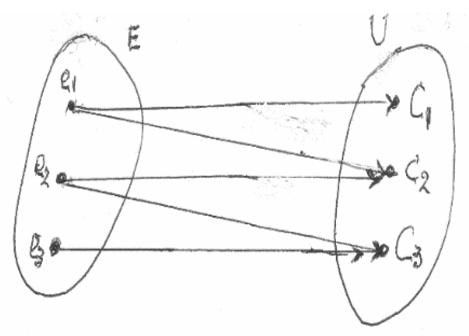
4.1. The Concept of Soft Set

In 1999, D. Molodstov, Professor of the Russian Academy of Sciences, introduced the notion of the soft set (SS) as a means for tackling uncertainty, in terms of a suitable set of parameters, in the following way [17]:

Definition 7.

Let E be a set of parameters, let A be a subset of E, and let f be a map from A into the power set P(U) of the universe U. Then the SS (f, A) in U has the form

(f, A) = {(e, f(e)): e ∈ A}

(5)

In other words, an SS can be considered as a parametrized family of subsets of U. The name “soft” is due to the fact that the form of (f, A) depends on the parameters of A. For each e ∈ A, its image f(e) in P(U) is called the value set of e in (f, A), while f is called the approximation function of (f, A).

For example, let U = {C₁, C₂, C₃} be a set of cars and let E = {e₁, e₂, e₃} be the set of the parameters e₁ = cheap, e₂ = hybrid (petrol and electric power), and e₃ = expensive. Let us further assume that C₁, C₂ are cheap, C₃ is expensive, and C₂, C₃ are the hybrid cars. Then, a map f: E $\to$ P(U) is defined by f(e₁) = {C₁, C₂}, f(e₂) = {C₂, C₃} and f(e₃) = {C₃}. Therefore, the SS (f, E) in U is the set of the ordered pairs (f, E) = {(e₁, {C₁, C₂}), (e₂, {C₂, C₃}, (e₃, {C₃}}. The SS (f, E) can be represented by the graph of Figure 2.

On comparing the graphs of Figure 1 and Figure 2, one can see that an FS is represented by a simple graph, whereas a bipartite graph [39] is needed for the representation of an SS.

Maji et al. [40] introduced a tabular representation of SSs in the form of a binary matrix in order to be stored easily in a computer’s memory. For example, the tabular representation of the soft set (f, E) is given in

Table 1. Tabular representation of the SS (f, E).

	e1	e2	e3
C1	1	0	0
C2	1	1	0
C3	0	1	1

.

An FS in U with the membership function y = m(x) is an SS in U of the form (f, [0, 1]), where

f(α) = {x $\in$ U: m(x) $\ge$ α} is the corresponding a-cut of the FS, for each α in [0, 1]. Consequently, the concept of SS is a generalization of the concept of FS.

An important advantage of SSs is that, by using the parameters, they pass through the already mentioned difficulty of properly defining membership functions.

4.2. Operations on Soft Sets

Definition 8.

The absolute SS A_U is the SS (f, A) in which f(e) = U,∀ e∈ A, and the null soft set A_∅ is the SS (f, A) in which f(e) =∅,∀ e∈A.

Definition 9.

If (f, A) and (g, B) are SSs in U, (f, A) is a soft subset of (g, B), if A $\subseteq$ B and f(e) $\subseteq$ g(e), ∀ e ∈ A. We write then (f, A) $\subseteq$ (g, B). If A $\subset$ B, then (f, A) is called a proper soft subset of B and we write (f, A) $\subset$ (g, B).

Definition 10.

Let (f, A) and (g, B) be SSs in U. Then:

• The union (f, A) ∪ (g, B) is the SS (h, A∪B) in U, with h(e) = f(e) if e∈ A-B, h(e) = g(e) if e∈ B-A and h(e) = f(e)∪g(e) if e∈ A∩B.
• The intersection (f, A) ∩ (g, B) is the soft set (h, A∩B) in U, with h(e) = f(e)∩g(e),∀ e∈ A∩B.
• The complement (f, A)^C of the soft SS (f, A) in U, is defined to be the SS (f*, A) in U, in which the function f* is defined by f*(e) = U−f(e),∀ e∈ A.

For general facts on soft sets, we refer to [41].

Example 1.

Let U = {H₁, H₂, H₃}, E = {e₁, e₂, e₃} and A = {e₁, e₂}. Consider the SS

S = (f, A) = {(e₁, {H₁, H₂}), (e₂, {H₂, H₃})} of U. Then the soft subsets of S are the following:

S₁ = {(e₁, {H₁})}, S₂ = {(e₁, {H₂})}, S₃ = {(e₁, {H₁, H₂})},

S₄ = {(e₂, {H₂})}, S₅ = {(e₂, {H₃})}, S₆ = {(e₂, {H₂, H₃})},

S₇ = {(e₁, {H₁}, (e₂, {H₂})}, S₈ = {(e₁, {H₁}, (e₂, {H₃})},

S₉ = {(e₁, {H₂}, (e₂, {H₂})}, S₁₀ = {(e₁, {H₂}, (e₂, {H₃})},

S₁₁ = {(e₁, {H₁, H₂}, (e₂, {H₂})}, S₁₂ = {(e₁, {H₁, H₂}, (e₂, {H₃})},

S₁₃ = {(e₁, {H₁}, (e₂, {H₂, H₃})}, S₁₄ = {(e₁, {H₂}, (e₂, {H₂, H₃})},

S, A_∅ = {(e₁,∅), (e₂,∅)}. It is also easy to check that (f, A)^C = {(e₁, {H₃}), (e₂, {H₁})}.

5. Hybrid Assessment and Decision Making Methods under Fuzzy Conditions

Each of the various theories that have been proposed for tackling existing real world uncertainty [19] is more suitable for certain types of uncertainty. Frequently, however, a combination of two or more of these theories gives better results. To support this argument, we present here two hybrid methods for assessment [42] and decision making [43] respectively under fuzzy conditions using SSs and closed real intervals as tools

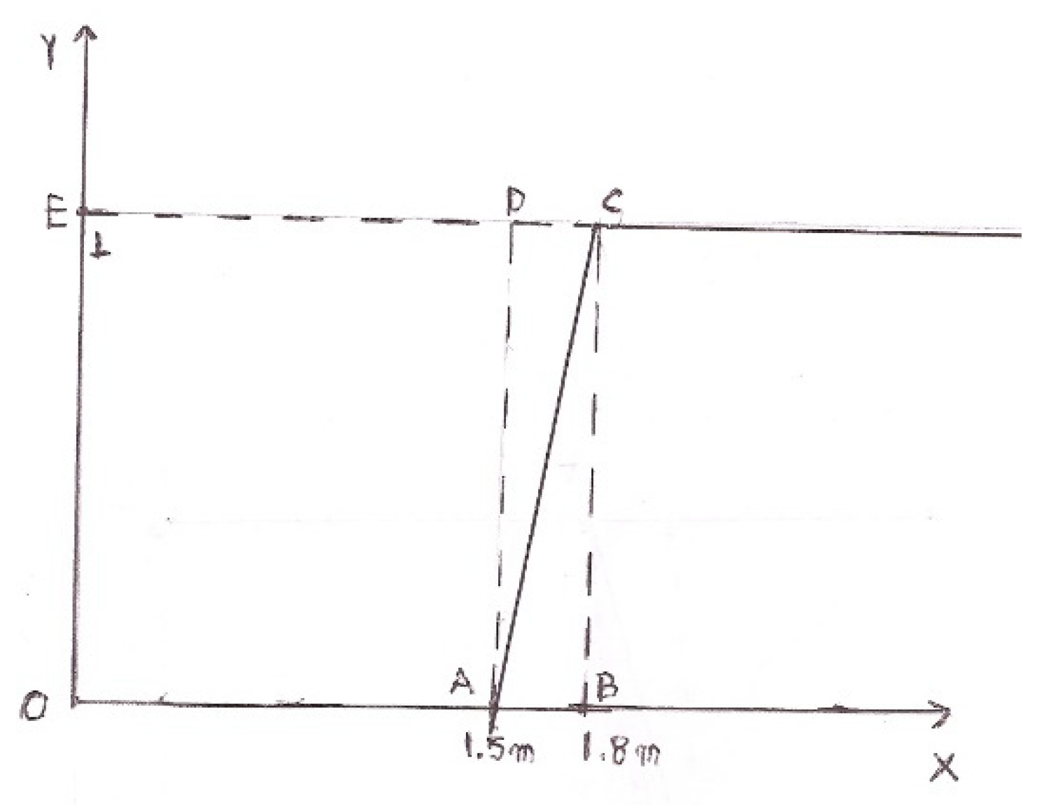
5.1. Using Closed Real Intervals for Handling Approximate Data

An important perspective of the closed intervals of real numbers is their use for handling approximate data. In fact, a numerical interval I = [x, y], with x, y real numbers, x < y, is actually representing a real number with a known range, whose exact value is unknown. When no other information is given about this number, it looks logical to consider, as its representative approximation, the real value

$$\mathrm{V}\left(\mathrm{I}\right)=\frac{\mathrm{x}+\mathrm{y}}{2}$$

(6)

The closer x to y, the better V(I) approximates the corresponding real number.

Moore et al. introduced in 1995 [44] the basic arithmetic operations on closed real intervals.

In particular, and according to the interests of the present article, if I₁ = [x₁, y₁] and I₂ = [x₂, y₂] are closed intervals, then their sum I₁ + I₂ is the closed interval

I₁ + I₂ = [x₁+ x₂, y₁+ y₂]

(7)

Also, if k is a positive number then the scalar product kI₁ is the closed interval

kI₁ = [kx₁, ky₁]

(8)

When the closed real intervals are used for handling approximate data, are also referred to as grey numbers (GNs). A GN [x, y], however, may also be connected with a whitenization function

f: [x, y] → [0, 1], such that, ∀ a ∈ [x, y], the closer f(a) to 1, the better the approximates of the unknown number represented by [x, y] ([22], Section 6.1).

We close this subsection about closed real intervals with the following definition, which will be used in the assessment method that follows.

Definition 11.

Let I₁, I₂,…., I_k be a finite number of closed real intervals and assume that I_i appears n_i times in an application, i = 1, 2, …., k. Set n = n₁ + n₂ + …. + n_k. Then the mean value of all these intervals is defined to be the closed real interval

$$\mathrm{I}=\frac{1}{\mathrm{n}} ({\mathrm{n}}_1{\mathrm{I}}_1+{\mathrm{n}}_2{\mathrm{I}}_2+\dots .{\mathrm{n}}_{\mathrm{k}}{\mathrm{I}}_{\mathrm{k}})$$

(9)

5.2. The Assessment Method

Assessment is one of the most important components of all human and machine activities, helping to determine possible mistakes and to improve performance with respect to a certain activity.

The assessment processes are realized by using either numerical or linguistic (qualitative) grades, such as excellent, good, moderate, etc. Traditional assessment methods are applied in the former case, which give accurate results, the most standard among them being the calculation of the mean value of the numerical scores.

Frequently, however, the use of numerical scores is either not possible (e.g., in the case of approximate data) or not desirable (e.g., when more elasticity is required for the assessment). In such cases, assessment methods based on principles of FL are usually applied. A great part of the present author’s earlier researches were focused on developing such kinds of methods, most of which are reviewed in detail in [22]. It seems, however, that proper combinations of the previous methodologies could give better results (e.g., see [42]). The assessment method developed by the present author in [42] will be illustrated here with the help of the following example.

Example 2.

Let U = {p₁, p₂,…, p₁₉, p₂₀} be the set of the players in a football team. Assume that the first 3 of them are excellent players, the next 7 very good players, the following 5 good players, the next 3 mediocre players, and the last 2 new players have no satisfactory performance yet. It is asked: (1) to make a parametric assessment of the team’s quality, and (2) to estimate the mean potential of the team.

Solution: (1) Consider the linguistic grades A = excellent, B = very good, C = good, D = mediocre, and F = not satisfactory, set E = {A, B, C, D, F} and define a map f: E → P(U) by f(A) = {p₁, p₂, p₃}, f(B) = {p_4, p₅, …,p₁₀}, f(C) = {p₁₁, p₁₂,…, p₁₅}, f(D) = {p₁₆, p₁₇, p₁₈}, and f(F) = {p₁₉, p₂₀}. Then the required parametric assessment of the team’s quality can be represented by the soft set

(f, E) = {(A, f(A)), (B, f(B)), (C, f(C)), (D, f(D)), (F, f(F))}

(2) Assign to each parameter (linguistic grade) of E a closed real interval, denoted for simplicity by the same letter, as follows: A = [85, 100], B = [75, 84], C = [60, 74], D = [50, 59], F = [0, 49]. Then by (9), the mean potential of the football team can be approximated by the real interval

$$\mathrm{M}=\frac{1}{20}(3\mathrm{A}+7\mathrm{B}+5\mathrm{C}+3\mathrm{D}+2\mathrm{F})$$

Applying Equations (7) and (8) and making the corresponding calculations one finds that

M = $\frac{1}{20}$[1230, 1533] = [61.5, 76.65]. Thus, Equation (5) gives that V(M) = 69.075, which shows that the mean potential of the football team is good (C).

Remark 1.

The choice of the intervals in case 2 of the previous example corresponds to generally accepted standards for translating the linguistic grades A, B, C, D, F in the numerical scale 0–100. By no means, however, should this choice be considered as being unique, since it depends on the special beliefs of the user. For example, one could as well choose A = [80, 100], B = [70, 79], C = [60, 69], D = [50, 59], F = [0, 49], etc.

Remark 2.

One could equivalently use triangular fuzzy numbers (TFNs) instead of closed real intervals in the previous example [22].

5.3. The Decision Making Method

Maji et al. [40] developed a parametric DM method using SSs as tools. In an earlier work [42], we have improved their method by adding closed real intervals (GNs) to the tools. Here, we illustrate our improved method with the following example.

Example 3.

A candidate buyer, who believes that the ideal house to buy should be cheap, beautiful, wooden and in the country, has to choose among six houses H₁, H₂, H₃, H₄, H₅ and H₆, which are for sale. Assume further that H₁, H₂, H₆ are the beautiful houses, H₂, H₃, H₅, H₆ are in the country, H₃, H₅ are wooden and H₄ is the unique cheap house. Which is the best choice for the candidate buyer?

Solution: First we solve this DM problem following the method of Maji et al. [40]. For this, consider U = {H₁, H₂, H₃, H₄, H₅, H₆} as the set of the discourse and let E = {e₁, e₂, e₃, e₄} be the set of the parameters e₁ = beautiful, e₂ = in the country, e₃ = wooden and e₄ = cheap. Then a map f: E → P(U) is defined by f(e₁) = { H₁, H₂, H₆}, f(e₂) = { H₂, H₃, H₅, H₆}, f(e₃) = { H₃, H₅}, f(e₄) = { H₄}, which gives rise to the SS (f, E) = {(e₁, f(e₁)), (e₂, f(e₂)), (e₃, f(e₃)), (e₄, f(e₄)}.

One can write the previous SS in its tabular form as it is shown in

Table 2. Tabular representation of the SS (f, E).

	e1	e2	e3	e4
H1	1	0	0	0
H2	1	1	0	0
H3	0	1	1	0
H4	0	0	0	1
H5	0	1	1	0
H6	1	1	0	0

.

Then, the choice value of each house is calculated by adding the binary elements of the row of Table 1 in which it belongs. The houses H₁ and H₄ have, therefore, choice value 1 and all the others have choice value 2. Consequently, the candidate buyer must choose one of the houses H₂, H₃, H₅ or H₆.

The previous decision, however, is obviously not so helpful. This gives us a hint to revise the previous DM method of Maji et al. In fact, observe that, in contrast to e₂ and e₃, the parameters e₁ and e₄ in the present problem do not have a bivalent texture. This means that it is closer to reality to characterize them using the qualitative grades A, B, C, D and F of Example 1, than by the binary elements 0, 1.

Assume, therefore, that the candidate buyer, after carefully studying all of the existing information about the six houses for sale, decided to use the following

Table 3. Revised tabular representation of the SS (f, E).

	e1	e2	e3	e4
H1	A	0	0	C
H2	A	1	0	F
H3	C	1	1	C
H4	D	0	0	A
H5	D	1	1	C
H6	A	1	0	D

instead of Table 2 to make the right decision.

From Table 3, one calculates the choice value C_i of the house Hi, i = 1, 2, 3, 4, 5, 6 as follows:

C₁ = V(A + C), or by (6) C₁ = V([0.85 + 0.6, 1 + 0.74]) and finally by (5) C₁ = $\frac{1.45+1.74}{2}$ = 1.595. Similarly, C₂ = 1 + V(A + F) = 1 + $\frac{0.85+1.49}{2}$ = 2.17, C₃ = 2 + V(C + C) = 3.34, C₄ = V(D + A) = 1.47, C₅ = 2 + V(D + C) = 3.215, and C₆ = 1 + V(A + D) = 2.47. The right decision is, therefore, to buy house H₃.

Remark 3.

One could, as in Example 2, use TFNs instead of closed real intervals [45] in this DM problem.

Remark 4.

The novelty of our hybrid DM method, with respect to the DM method of Maji et al. [40], is that, by using closed real intervals instead of the binary elements 0, 1 in the tabular matrix of the corresponding SS in cases where some (or all) of the parameters are not of bivalent texture, we succeed in making a better decision.

5.4. Weighted Decision Making

When the goals put by the decision-maker are not of the same importance, weight coefficients must be assigned to each parameter to make the proper decision. Assume, for instance, that in the previous example the candidate buyer assigned the weight coefficients 0.9 to e₁, 0.7 to e₂, 0.6 to e₃ and 0.5 to e₄. Then, the weighted choice values of the houses in Example 3 are calculated as follows:

C₁ = V(0.9A + 0.5C), or by (5), (6) and (7) C₁ = V([1.65, 1.27]) = 1.46. Similarly, C₂ = 0.7 + V(0.9A + 0.5F) = 0.7 + V([0.765,1.145]) = 1.655, C₃ = 0.7 + 0.6 + V(0.9C + 0.5C) = 1.3 + V([0.84,1.036]) = 2.238, C₄ = V(0.9D + 0.5A) = V([0.875,1.031]) = 0.953, C₅ = 0.7 + 0.6 + V(0.9D + 0.5C) = 1.3 + V([0.75, 0.901]) = 2.1255, C₆ = 0.7 + V(0.9A + 0.5D) = 0.7 + V([1.015, 1.195]) = 1.805. Consequently, the right decision is, again, to buy house H₃.

6. Topological Spaces in Fuzzy Structures

TSs is the most general category of mathematical spaces, in which fundamental mathematical notions are defined [46]. In this section, we describe how the concept of TS is extended to fuzzy structures.

6.1. Fuzzy Topological Spaces

Definition 12

([25]).A fuzzy topology (FT) T on a non-empty set U is a family of FSs in U such that:

• The universal and the empty FSs belong to T;
• The intersection of any two elements of T and the union of an arbitrary number (finite or infinite) of elements of T also belong to T.

Trivial examples of FTs are the discrete FT {F_∅, F_U} and the non-discrete FT of all FSs in U. Another example is the set of all constant FSs in U, i.e., all FSs in U with a membership function defined by m(x) = c, for some c in [0, 1], and all x in U.

The elements of an FT T on U are referred to as fuzzy open sets in U and their complements are referred to as fuzzy closed sets in U. The pair (U, T) is called a fuzzy topological space (FTS) on U.

Next, it is described how the fundamental notions of limit, continuity, compactness, and Hausdorff TS can be extended to FTSs [25].

Definition 13.

Given two FSs A and B of the FTS (U, T), B is called a neighborhood of A, if there exists an open FS O such that A $\subseteq$ O $\subset$ B.

Definition 14.

A sequence {A_n} of FSs of (U, T) converges to the FS A of (U, T), if there exists a positive integer m, such that for each integer n ≥ m and each neighborhood B of A we have that A_n $\subset$ B. Then A is said to be the limit of {A_n}.

Lemma 1.

(Zadeh’s extension principle.) Let X and Y be two non-empty crisp sets and let f: X $\to$ Y be a function. Then f is extended to a function F mapping FSs in X to FSs in Y.

Proof. 

Let A be an FS in X with a membership function m_A. Then, its image F(A) is an FS B in Y with a membership function m_B, which is defined as follows: Given y in Y, consider the set f ⁻¹(y) = {x ∈ X: f(x) = y}. If f ⁻¹(y) = ∅, then m_B(y) = 0, and if f ⁻¹(y) ≠ ∅, then m_B(y) = max {m_A(x): x ∈ f ⁻¹(y)}. Conversely, the inverse image F⁻¹(B) is the FS A in X with a membership function m_A(x) = m_B(f(x)), for each x ∈ X. □

Definition 15.

Let (X, T) and (Y, S) be two FTSs and let f: X $\to$ Y be a function. Then f is extended to a function F mapping FSs in X to FSs in Y. Then f is said to be a fuzzily continuous function, if, and only if, the inverse image of each open FS in Y through F is an open FS in X.

Definition 16.

A family A = {A_i, i∈I} of FSs of an FTS (U, T) is said to be a cover of U, if U = ${\displaystyle \underset{\mathrm{i}\in \mathrm{I}}{\cup }{\mathrm{A}}_{\mathrm{i}}}$. If the elements of A are open FSs, then A is said to be an open cover of U. A subset of A, which is also a cover of U, is called a sub-cover of A. The FTS (U, T) is said to be compact, if every open cover of U contains a sub-cover with many finite elements.

Definition 17.

An FTS (U, T) is said to be:

• A T₁-FTS, if, and only if, for each pair of elements u₁, u₂ of U, u₁ ≠ u₂, there exist at least two open FSs O₁ and O₂ such that u₁∈O₁, u₂ $\notin$O₁ and u₂∈O₂, u₁ $\notin$ O₂.
• A T₂-FTS (or a separable or Hausdorff FTS), if, and only if, for each pair of elements u₁, u₂ of U, u₁ ≠ u₂, there exist at least two open FSs O₁ and O₂ such that u₁∈O₁, u₂∈O₂ and O₁∩O₂ =∅_F.

Obviously a T₂-FTS is always a T₁-FTS.

6.2. Soft Topological Spaces

Observe that the concept of FTS (Definition 12) is obtained from the classical definition of TS [45] by replacing the statement “a family of subsets of U” by the statement “a family of FSs in U”. In an analogous way, one can obtain the concepts of intuitionistic FTS (IFTS) [26], of neutrosophic TS (NTS) [47], of soft TS (STS) [48], etc. In particular, an STS is defined as follows:

Definition 18.

A soft topology T on a non-empty set U is a family of SSs in U with respect to a set of parameters E such that:

• The absolute and S null soft sets E_U and E_∅ belong to T;
• The intersection of any two elements of T and the union of an arbitrary number (finite or infinite) of elements of T also belong to T.

The elements of an ST T on U are said to be open SS and their complements are said to be closed SS. The triple (U, T, E) is said to be an STS on U.

Trivial examples of STs are the discrete ST {E_∅, E_U} and the non-discrete ST of all SSs in U. Reconsider also Example 1. It is straightforward to check then that T = {E_U, E_∅, S, S₂, S₉, S₁₁} is ST on U.

The concepts of limit, continuity, compactness, and Hausdorff TS are extended to STs in a way analogous to FTSs [49,50]. In fact, Definitions 13, 14, 16 and 17 are easily turned to corresponding definitions of STSs by replacing the expression “fuzzy sets” with the expression “soft sets”. For the concept of continuity, we need the following Lemma ([49], definition 3.12):

Lemma 2.

Let (U, T, A), (V, S, B) be STSs and let u: U → V, p: A → B be given maps. Then a map f_pu is defined with respect to u and p mapping the soft sets of T to soft sets of S.

Proof. 

If (F, A) is a soft set of T, then its image f_pu((F, A)) is a soft set of S defined by

f_pu((F, A)) = (f_pu(F), p(A)), where, ∀ y ∈ B is f_pu(F)(y) = ${\displaystyle \underset{\mathrm{x}\in {\mathrm{p}}^{-1}\left(\mathrm{y}\right)\cap \mathrm{A}}{\cup }\mathrm{u}\left(\mathrm{F}\right(\mathrm{x}\left)\right)}$ if p⁻¹(y)∩A≠∅ and f_pu(F)(y) = ∅ otherwise. □

Conversely, if (G, B) is a soft set of S, then its inverse image f_pu⁻¹((G, B)) is a soft set of T defined by f_pu⁻¹((G, B)) = (f_pu⁻¹(G), p⁻¹(B)), where ∀ x ∈ A is

f_pu⁻¹(G)(x) = u⁻¹(G(p(x)).

Definition 19.

Let (U, T, A), (V, S, B) be STSs and let u: U → V, p: A → B be given maps. Then the map f_pu, defined by Lemma 2, is said to be soft pu-continuous, if, and only if, the inverse image of each open soft set in Y through f_pu is an open soft set in X.

7. Discussion and Conclusions

Three were the goals of the present review paper:

• We came across the main steps that were laid from Zadeh’s FS and Atanassov’s IFS to Smarandache’s NS and to Molodstov’s SS.
• We presented, using suitable examples, two recently developed by us hybrid methods for assessment and DM, respectively, using SSs and closed real intervals (GNs) as tools.
• We described how one can extend the concept of TS to fuzzy structures and how we can define limits, continuity, compactness and Hausdorff spaces on those structures. In particular, FTSs and STSs were defined, and characteristic examples were presented.

For reasons of completeness, however, we ought to note that, despite the fact that IFSs and SSs have already found many and important applications, there exist reports in the literature disputing the significance of these concepts, and in extension, of the notions of IFSTS and STs, considering them as redundant, representing an unnecessarily complicated way, a standard fixed-basis set theory and topology [51,52,53,54]. In the Abstract of [52], for example, one reads: “In particular, a soft set on X with a set E of parameters actually can be regarded as a 2E-fuzzy set or a crisp subset of E × X [the correct is E × P(X)]. This shows that the concept of (fuzzy) soft set is redundant”. I completely disagree with this way of thinking. Adopting it, one could claim that, since an FS A in X is a subset of the Cartesian product X × m(X), where m is the membership function of A, the concept of FS is redundant!

Among probability, FSs and the other related generalizations and theories [19], there is not an ideal model for effectively tackling all the existing types of real world uncertainty. Each one of these theories is more suitable for dealing with special types of uncertainty, e.g., probability for randomness, FSs for vagueness, IFSs for imprecision in human thinking, NSs for ambiguity and inconsistency, etc. All these theories together, however, provide an adequate framework for managing the uncertainty.

Even more, it seems that proper combinations of the previous theories give frequently better results, not only for tackling the existing uncertainty, but also for assessment purposes [42], for DM under fuzzy conditions [43], and possibly for various other human and machine activities. This is, therefore, a promising area for future research.

As we have mentioned in our Introduction, the concept of the ordinary FS, otherwise termed as type-1 FS, was generalized to the type-2 FS and further to type-n FS, n ≥ 2, so that more uncertainty can be handled and connected to the membership function [8]. The membership function of a type-2 FS is three-dimensional, its third dimension being the value of the membership function at each point of its two-dimensional domain, which is called the footprint of uncertainty (FOU). The FOU is completely determined by its two bounding functions, a lower membership function and an upper membership function, both of which are type-1 FSs. When no uncertainty exists about the membership function, then a type-2 FS reduces to a type-1 FS, in a way analogous to probability reducing to determinism when unpredictability vanishes. However, when Zadeh proposed the type-2 FS in 1975 [8], the time was not right for researchers to drop what they were doing with type-1 FS and focus on type-2 FS. This changed in the late 1990s as a result of Prof. Jerry Mendel’s works on type-2 FS and logic [55]. Since then, more and more researchers around the world are writing articles about type-2 FS and systems, while some important applications of type-3 FS and logic were also reported recently, e.g., [56,57]. This is, therefore, another promising area for future research.

References

1. Zadeh, L.A. Fuzzy Sets. Inf. Control 1965, 8, 338–353. [Google Scholar] [CrossRef] [Green Version]
2. Zadeh, L.A. Outline of a new approach to the analysis of complex systems and decision processes. IEEE Trans. Syst. Man Cybern. 1973, 3, 28–44. [Google Scholar] [CrossRef] [Green Version]
3. Zadeh, L.A. Fuzzy Sets as a basis for a theory of possibility. Fuzzy Sets Syst. 1978, 1, 3–28. [Google Scholar] [CrossRef]
4. Dubois, D.; Prade, H. Possibility theory, probability theory and multiple-valued logics: A clarification. Ann. Math. Artif. Intell. 2001, 32, 35–66. [Google Scholar] [CrossRef]
5. Dubois, D.; Prade, H. Possibility theory and its applications: A retrospective and prospective view. In Decision Theory and Multi-Agent Planning; Della Riccia, G., Dubois, D., Kruse, R., Lenz, H.J., Eds.; CISM International Centre for Mechanical Sciences (Courses and Lectures); Springer: Vienna, Austria, 2006; Volume 482. [Google Scholar]
6. Klir, G.J.; Folger, T.A. Fuzzy sets, Uncertainty and Information; Prentice-Hall: London, UK, 1988. [Google Scholar]
7. Kosko, B. Fuzziness Vs. Probability. Int. J. Gen. Syst. 1990, 17, 211–240. [Google Scholar] [CrossRef]
8. Zadeh, L.A. The Concept of a Linguistic Variable and its Application to Approximate Reasoning. Inf. Sci. 1975, 8, 199–249. [Google Scholar] [CrossRef]
9. Dubois, D.; Prade, H. Interval-Valued Fuzzy Sets, Possibility Theory and Imprecise Probability. Proc. EUSFLAT-LFA 2005, 1, 314–319. [Google Scholar]
10. Atanassov, K.T. Intuitionistic Fuzzy Sets. Fuzzy Sets Syst. 1986, 20, 87–96. [Google Scholar] [CrossRef]
11. Torra, V.; Narukawa, Y. On hesitant fuzzy sets and decision. In Proceedings of the 18th IEEE International Conference on Fuzzy Systems, Jeju, Korea, 20–24 August 2009; Volume 544, pp. 1378–1382. [Google Scholar]
12. Yager, R.R. Pythagorean fuzzy subsets. In Proceedings of the Joint IFSA World Congress and NAFIPS Annual Meeting, Edmonton, AB, Canada, 24–28 June 2013; pp. 57–61. [Google Scholar]
13. Smarandache, F. Neutrosophy/Neutrosophic Probability, Set, and Logic; ProQuest: Ann Arbor, MI, USA, 1998. [Google Scholar]
14. Ramot, D.; Milo, R.; Friedman, M.; Kandel, A. Complex fuzzy sets. IEEE Trans. Fuzzy Syst. 2002, 10, 171–186. [Google Scholar] [CrossRef]
15. Deng, J. Control Problems of Grey Systems. Syst. Control Lett. 1982, 1, 288–294. [Google Scholar]
16. Pawlak, Z. Rough Sets: Aspects of Reasoning about Data; Kluer Academic Publishers: Dordrecht, The Netherlands, 1991. [Google Scholar]
17. Molodtsov, D. Soft set theory—First results. Comput. Math. Appl. 1999, 37, 19–31. [Google Scholar] [CrossRef] [Green Version]
18. Cuong, B.C. Picture Fuzzy Sets. J. Comput. Sci. Cybern 2014, 30, 409–420. [Google Scholar]
19. Voskoglou, M.G. Generalizations of Fuzzy Sets and Related Theories. In An Essential Guide to Fuzzy Systems; Voskoglou, M., Ed.; Nova Science Publishers: Hauppauge, NY, USA, 2019; pp. 345–352. [Google Scholar]
20. Voskoglou, M.G. Finite Markov Chain and Fuzzy Logic Assessment Models: Emerging Research and Opportunities; Createspace. com–Amazon: Columbia, SC, USA, 2017. [Google Scholar]
21. Voskoglou, M.G. Fuzzy Control Systems. WSEAS Trans. Syst. 2020, 19, 295–300. [Google Scholar] [CrossRef]
22. Voskoglou, M.G. Methods for Assessing Human-Machine Performance under Fuzzy Conditions. Mathematics 2019, 7, 230. [Google Scholar] [CrossRef] [Green Version]
23. Tripathy, B.K.; Arun, K.R. Soft Sets and Its Applications. In Handbook of Research on Generalized and Hybrid Set Structures and Applications for Soft Computing; Jacob, J.S., Ed.; IGI Global: Hersey, PA, USA, 2016; pp. 65–85. [Google Scholar]
24. Kharal, A.; Ahmad, B. Mappings on soft classes. New Math. Nat. Comput. 2011, 7, 471–481. [Google Scholar] [CrossRef]
25. Chang, S.L. Fuzzy topological spaces. J. Math. Anal. Appl. 1968, 24, 182–190. [Google Scholar] [CrossRef] [Green Version]
26. Luplanlez, F.G. On Intuitionistic Fuzzy Topological Spaces. Kybernetes 2006, 35, 743–747. [Google Scholar]
27. Zadeh, L.A. Fuzzy logic = computing with words. IEEE Trans. Fuzzy Syst. 1996, 4, 103–111. [Google Scholar] [CrossRef] [Green Version]
28. Voskoglou, M.G. Managing the Uncertainty: From Probability to Fuzziness, Neutrosophy and Soft Sets. Trans. Fuzzy Sets Syst. 2022, 1, 46–58. [Google Scholar] [CrossRef]
29. Jaynes, E.T. Probability Theory: The Logic of Science; 8th Printing; Cambridge University Press: Cambridge, UK, 2011. [Google Scholar]
30. Mumford, D. The Dawning of the Age of Stochasticity. In Mathematics: Frontiers and Perspectives; Amoid, V., Atiyah, M., Laxand, P., Mazur, B., Eds.; AMS: Providence, RI, USA, 2000; pp. 197–218. [Google Scholar]
31. Voskoglou, M.G. The Importance of Bayesian Reasoning in Every Day Life and Science. Int. J. Educ. Dev. Soc. Technol. 2020, 8, 24–33. [Google Scholar]
32. Gentili, P.L. Establishing a New Link between Fuzzy Logic, Neuroscience, and Quantum Mechanics through Bayesian Probability: Perspectives in Artificial Intelligence and Unconventional Computing. Molecules 2021, 26, 5987. [Google Scholar] [CrossRef]
33. Bertsch McGrayne, S. The Theory That Would Not Die; Yale University Press: New Haven, CT, USA; London, UK, 2012. [Google Scholar]
34. What Do You Think about Machines That Think? 2015. Available online: http://edge.org/response-detail/26871 (accessed on 24 March 2022).
35. Jeffreys, H. Scientific Inference, 3rd ed.; Cambridge University Press: Cambridge, UK, 1973. [Google Scholar]
36. Atanassov, K.T. Intuitionistic Fuzzy Sets; Physica-Verlag: Heidelberg, Germany, 1999. [Google Scholar]
37. Smarandache, F. Indeterminacy in Neutrosophic Theories and their Applications. Int. J. Neutrosophic Sci. 2021, 15, 89–97. [Google Scholar] [CrossRef]
38. Wang, H.; Smarandanche, F.; Zhang, Y.; Sunderraman, R. Single Valued Neutrosophic Sets. Rev. Air Force Acad. 2010, 1, 10–14. [Google Scholar]
39. Farid, F.; Saeed, M.; Ali, M. Representation of Soft Set and its Operations by Bipartite Graph. Sci. Inq. Rev. 2019, 3, 30–42. [Google Scholar] [CrossRef]
40. Maji, P.K.; Roy, A.R.; Biswas, R. An Application of Soft Sets in a Decision Making Problem. Comput. Math. Appl. 2002, 44, 1077–1083. [Google Scholar] [CrossRef] [Green Version]
41. Maji, P.K.; Biswas, R.; Ray, A.R. Soft Set Theory. Comput. Math. Appl. 2003, 45, 555–562. [Google Scholar] [CrossRef]
42. Voskoglou, M.G.; Broumi, S. A Hybrid Method for the Assessment of Analogical Reasoning Skills. J. Fuzzy Ext. Appl. 2022, 3, 152–157. [Google Scholar]
43. Voskoglou, M.G. A Combined Use of Softs Sets and Grey Numbers in Decision Making. J. Comput. Cogn. Eng. 2022, in press. [Google Scholar] [CrossRef]
44. Moore, R.A.; Kearfort, R.B.; Clood, M.G. Introduction to Interval Analysis, 2nd ed.; SIAM: Philadelphia, PA, USA, 1995. [Google Scholar]
45. Voskoglou, M.G. A Hybrid Model for Decision Making Utilizing TFNs and Soft Sets as Tools. Equations 2022, 2, 65–69. [Google Scholar] [CrossRef]
46. Willard, S. General Topology; Dover Publ. Inc.: Mineola, NY, USA, 2004. [Google Scholar]
47. Salama, A.A.; Alblowi, S.A. Neutrosophic Sets and Neutrosophic Topological Spaces. IOSR J. Math. 2013, 3, 31–35. [Google Scholar] [CrossRef]
48. Shabir, M.; Naz, M. On Soft Topological Spaces. Comput. Math. Appl. 2011, 61, 1786–1799. [Google Scholar] [CrossRef] [Green Version]
49. Zorlutuna, I.; Akdag, M.; Min, W.K.; Amaca, S. Remarks on Soft Topological Spaces. Ann. Fuzzy Math. Inform. 2011, 3, 171–185. [Google Scholar]
50. Georgiou, D.N.; Megaritis, A.C.; Petropoulos, V.I. On Soft Topological Spaces. Appl. Math. Inf. Sci. 2013, 7, 1889–1901. [Google Scholar] [CrossRef]
51. Garcia, J.; Rodabaugh, S.E. Order-theoretic, topological, categorical redundancies of interval-valued sets, grey sets, vague sets, interval-valued “intuitionistic” sets, “intuitionistic” fuzzy sets and topologies. Fuzzy Sets Syst. 2005, 156, 445–484. [Google Scholar] [CrossRef]
52. Shi, F.G.; Fan, C.Z. Fuzzy soft sets as L-fuzzy sets. J. Intell. Fuzzy Syst. 2019, 37, 5061–5066. [Google Scholar] [CrossRef]
53. Shi, F.G.; Pang, B. Redundancy of fuzzy soft topological spaces. J. Intell. Fuzzy Syst. 2014, 27, 1757–1760. [Google Scholar] [CrossRef]
54. Shi, F.G.; Pang, B. A note on soft topological spaces. Iran. J. Fuzzy Syst. 2015, 12, 149–155. [Google Scholar]
55. Mendel, J.M. Uncertain Rule-Based Fuzzy Logic Systems: Introduction and New Directions; Prentice-Hall: Upper-Saddle River, NJ, USA, 2001. [Google Scholar]
56. Mohammadzadeh, A.; Sabzalian, M.H.; Zhang, W. An interval type-3 fuzzy system and a new online fractional-order learning algorithm: Theory and practice. IEEE Trans. Fuzzy Syst. 2020, 28, 1940–1950. [Google Scholar] [CrossRef]
57. Cao, Y.; Raise, A.; Mohammadzadeh, A.; Rathinasamy, S.; Band, S.S.; Mosavi, A. Deep learned recurrent type-3 fuzzy system: Application for renewable energy modeling/prediction. Energy Rep. 2021, 7, 8115–8127. [Google Scholar] [CrossRef]
Figure 1. Graph of the FS of “tall people”.
Mathematics 10 03909 g001
Figure 2. Graphical representation of the SS (f, E).
Mathematics 10 03909 g002