Article

Multifractal Characteristics on Temporal Maximum of Air Pollution Series

by
Nurulkamal Masseran
Department of Mathematical Sciences, Faculty of Science and Technology, Universiti Kebangsaan Malaysia, Bangi 43600, Selangor, Malaysia
Mathematics 2022, 10(20), 3910; https://doi.org/10.3390/math10203910
Submission received: 5 September 2022 / Revised: 14 October 2022 / Accepted: 19 October 2022 / Published: 21 October 2022
(This article belongs to the Special Issue Data Analysis and Domain Knowledge)

Abstract

:
Presenting and describing a temporal series of air pollution data with longer time lengths provides more concise information and is, in fact, one of the simplest techniques of data reduction in a time series. However, this process can result in the loss of important information related to data features. Thus, the purpose of this study is to determine the type of data characteristics that might be lost when describing data with different time lengths corresponding to a process of data reduction. In parallel, this study proposes the application of a multifractal technique to investigate the properties on an air pollution series with different time lengths. A case study has been carried out using an air pollution index data in Klang, Malaysia. Results show that hourly air pollution series contain the most informative knowledge regarding the behaviors and characteristics of air pollution, particularly in terms of the strength of multifractality, long-term persistent correlations, and heterogeneity of variations. On the other hand, the statistical findings found that data reduction corresponding to a longer time length will change the multifractal properties of the original data.

1. Introduction

Air pollution is among the important issues that need to be addressed by all countries due to its impact on many aspects of human life, particularly on health [1,2], economics [3,4], and environmental sustainability [5]. This scenario is even more critical to address in urban areas [6,7] given their dense populations and active economic activities, with needs for sustainable development and better living welfare or infrastructure for the community. However, dense populations and active economic activities lead to increasing air pollution particularly due to mobile (motor vehicles) and stationary sources (power stations and industrial fuel burning and processes) [8]. Thus, managing and controlling the adverse effects of air pollution in urban areas always need regulation. For this purpose, the monitoring and assessment of air pollution behaviors over time is an important task.
One of the most important processes in monitoring and assessing air pollution behaviors is the analysis of recorded air pollution data over time. Most of the available literature investigates the behaviors of air pollution data using various statistical models, including the time series approach [9,10,11,12], regression technique [13,14], stochastic analysis [15,16], distribution models [17,18,19], neural network and deep learning [20,21,22], spatial-temporal [23,24,25], extreme-value analysis [26,27], and multivariate approach [28,29]. All of these methods provide valuable information about the behaviors, trends, and dependency structures of air pollution characteristics. However, these commonly used statistical models may show biases and uncertainties with regard to different temporal scales in describing an air pollution series. With the aim to reduce biases and uncertainties, the past and current air pollution data must be evaluated according to several relevant parameters [30,31]. Thus, another approach is investigating the behavior of air pollution events by assessing their degree of nonlinearity and overall process complexity. This objective can be achieved by employing nonlinear techniques, such as information entropy measures [32,33], fractal and multifractal analysis [34,35], chaotic analysis [36], and complex networks [37]. In parallel, this study focuses on the application of multifractal analysis to provide empirical evidence on behaviors and characteristics of air pollution series in different time lengths by means of fractal geometry.
The available literature related to multifractal analysis on air pollution mostly focuses on investigating the existence of multifractality characteristics and long-term cross-correlations series within and between several locations. For example, several researchers such as Wang et al. [30], Chen-hua et al. [38], Liu et al. [39], and Xu et al. [40] adopt the multifractal technique to analyze the multifractal characteristics of air pollution series for several cities in China. In general, their results found that long-range correlations and fat-tail distribution are the main sources that reflect the characteristics of air pollution in China. In fact, different pollutant variables are found to have a different impact on air quality in different locations. In parallel, a similar analysis related to the investigation of multifractality characteristics on air pollution data has also been done by researchers around the world, such as in India [41], Mexico [42], Malaysia [43], the Caribbean basin [44], etc. In addition, multifractal analysis has been used to find out the impact of air pollution events related to health [45], public policy [46], meteorological factors [47], and many more. However, there is no specific study that has been done to investigate the changing behaviors of multifractal characteristics on air pollution data with different time lengths. Particularly, a modified different time length corresponds to a process of data reduction. Thus, the main contribution of this study is to fill this gap by determining the characteristics of data that might be lost due to the process of data reduction corresponding to presenting and describing a data series with a longer time length.
This paper is organized as follows. Section 2 describes the study area and data. Section 3 describes the multifractal spectrum analysis technique used in this study, while Section 4 describes the multifractality characteristics. Next, the results and discussion are described in Section 5. In Section 6, some conclusions are drawn.

2. Study Area and Data

Klang is an urban area located at latitude 101°26′44.023″ E and longitude 3°2′41.701″ N in Peninsular Malaysia. Figure 1 shows the specific location. Klang plays important roles as an economic and industrial center in Malaysia, particularly as a trans-shipment port. In fact, this area has been recognized as the 13th busiest trans-shipment port and the 16th busiest container port in the world [48]. Among the most populated urban areas in the country, Klang also shows a very high density of motor vehicles used. Thus, Klang is exposed to a high risk of air pollution events compared with other areas [49]. Therefore, considering Klang as an important city in Malaysia, the analysis and monitoring of its air pollution behavior is highly significant and may provide useful information.
This study investigates the data of an air pollutant index (API) series in Klang for the period of 1 January 2002 to 31 August 2020. The API data are determined by integrating five primary pollutant variables, namely, suspended particulate matter with sizes less than 10 microns (PM10), nitrogen dioxide (NO2), ozone (O3), sulfur dioxide (SO2), and carbon monoxide (CO). Figure 2 shows the details. The Department of Environment Malaysia uses API as an indicator of the status of air quality at a particular time. In general, a high API indicates poor air quality [51]. Details regarding the calculation of API data can be referred to in Masseran and Safari [52] and Masseran [53].

3. Multifractal Spectrum Analysis

Multifractal Detrended Fluctuation Analysis (MFDFA) is a useful method in providing spectrum analysis on time series data. In this study, for an observed API series with the length { y ( t ) } , t = 1 , 2 , , N , the signal profile series is determined as:
Y ( i ) = t = 1 i ( y ( t ) y ¯ ) , i = 1 , 2 , , N
where y ¯ = t = 1 N y ( t ) / N is the mean. Then, a profile series Y ( i ) is partitioned into N s = [ N / s ] non-overlapping segments with a length s. However, if the length N is not an integral multiple in terms of scale s, then a certain portion of data points in the profile is unused. Given this problem, a solution construction is repeated starting from the opposite end of the dataset [54]. Thus, a profile with a total of 2 N s segments is used in multifractal analysis. On this basis, a local trend on each 2 N s segment needs to be determined by fitting the m-th order of the polynomial curve, given as:
Y v ( i ) = a ^ 0 + a ^ 1 i + a ^ 2 i 2 + + a ^ m i m , i = 1 , 2 , , s ,
where Y v ( i ) is the m-th polynomial order in segment v and is also known as an m-order of MFDFA. Equation (2) represents the local trend function on the v-th segment polynomial of the profile in terms of a constant (m = 0), linear (m = 1), quadratic (m = 2), or any higher-order trends [55]. Then, the variance for each segment in v = 1 , 2 , , N s can be computed as:
F 2 ( s , v ) = i = 1 s { Y [ ( v 1 ) s + i ] Y v ( i ) } 2 s .
Likewise, the variance for each segment in v = N s + 1 , , , 2 N s can be computed as:
F 2 ( s , v ) = i = 1 s { Y [ N ( v N s ) s + i ] Y v ( i ) } 2 s ,
where Y v ( i ) is the fitted m-th polynomial order in segment v. Another important information that needs to be derived is a q-order fluctuation function, which is determined by averaging F 2 ( s , v ) over all segments. For particular cases with q = 0 , the q-order fluctuation function is obtained as:
F 0 ( s ) = exp v = 1 2 N s ln [ F 2 ( s , v ) ] 4 N s ,
while for general cases with q 0 , the q-order fluctuation function can be obtained as:
F q ( s ) = { v = 1 2 N s [ F 2 ( s , v ) ] q 2 2 N s } 1 q .
Different q values have varying effects on the fluctuation functions. If q takes a positive value, then the segment v dominates the average of F q ( s ) with a large variance that indicates a large deviation from the corresponding fit. This case implies a scale invariance of the segments with large fluctuations as shown by positive q moments. Likewise, a scale invariance of the segments with small fluctuations are indicated by negative q moments [55].

4. Multifractality Characteristics

From Equations (5) and (6), if the air pollution series is found to be power-law correlated with an increasing value of s, then the series follows a power-law principle that can be described as:
F q ( s ) = s h ( q ) ,
where h ( q ) is a generalized Hurst exponent, the solution for which h ( q ) is obtained by implying the ln ( . ) function on Equation (7). Thus, the slope of ln [ F q ( s ) ] and ln ( s ) denotes the value h ( q ) , which provides information about the scaling behavior of the time series under study. If the h ( q ) function is independent of q moments, then the series is monofractal; if the h ( q ) function indicates a dependency on its q moments, then the series is multifractal. Apart from that, h ( q ) can be related to the Rényi exponent by the following equation [56].
τ ( q ) = q h ( q ) 1 ,
where τ ( q ) represents the Rényi exponent. The τ ( q ) function indicates a nonlinear relationship on q moments for the multifractal series, whereas a linear function appears for the monofractal series. The Rényi exponent provides information about the singularity spectrum, f ( α ) . By using a Legendre transformation, the relationship between τ ( q ) and f ( α ) can be obtained as:
α = d τ ( q ) d q ,
f ( α ) = q ( α ) τ ( q ) .
Based on Equation (8–10), the singularity spectrum can be determined as:
α = h ( q ) + q h ( q ) ,
f ( α ) = q ( α h ( q ) ) + 1 ,
where α is a Lipschitz–Hölder exponent that represents the singularity strength [57]. For a multifractal series, the singularity spectrum indicates a single humped function, while the monofractal series is represented by a single point in the f ( α ) plane [34]. Commonly, the complexity of the time series quantified by the measure of singularity spectra can be described by the fourth degree of the polynomial [58], determined as:
f ( α ) = A + B ( α α 0 ) + C ( α α 0 ) 2 + D ( α α 0 ) 3 + E ( α α 0 ) 4 ,
where α 0 is the value corresponding to the maximum of the spectrum, while the terms A, B, C, D, and E are coefficient parameters. The difference in terms of the singularity spectrum can be determined as:
Δ f ( α ) = f ( α min ) f ( α max ) ,
where Δ f ( α ) represents the differences between maximum and minimum values of the singularity that estimate the spread of the changes in the fractal patterns. In fact, Δ f ( α ) denotes the frequency ratio of the largest to the smallest fluctuation. Δ f ( α ) > 0 implies that large fluctuations occur more frequently than small ones. Conversely, Δ f ( α ) < 0 implies that the small fluctuations occur more frequently than large ones [55].
In addition, the strength of the multifractality is reflected by the spectrum width, which is determined as:
Δ α = α max α min = h ( ) h ( ) ,
given that
h ( q ) = 1 q ln ( a q + b q ) q ln ( 2 ) , ( a > b ) ,
where a and b are the parameters that need estimation. Generally, a large value of Δ α implies a stochastic dynamic character [59] and long-term series persistence [60]. Moreover, a large or small multifractal signal can be depicted by the value of Δ α , which implies a high or low heterogeneous signal. As described by Hou et al. [55], a signal characterized by sudden bursts of high frequency, intermittencies, and/or irregularities is heterogeneous. The other indices that can be used to describe the characteristics of multifractality in air pollution series are given as:
Δ α L = α 0 α min ,
Δ α R = α max α ,
where α 0 is the maxima position in the singularity spectrum, α max and α min are the maximum and minimum values of the Hölder exponent, respectively. The determined values of Δ α L and Δ α R provide information regarding the left- and right-hand branches of the singularity spectrum curve, which describes the distribution patterns of the high and low fluctuations, respectively [61]. Next, the deviations of the singularity spectrum curve can be determined using the asymmetry index, given as:
R = Δ α L Δ α R Δ α L + Δ α R ,
where the index R is in the range from −1 to 1 [62]. The value of R = 0 indicates a symmetrical singularity spectrum characteristic. If R > 0, then the series likely has a left-hand deviation of the singularity spectrum due to a certain degree of local high fluctuations. Conversely, a right-hand deviation with local low fluctuations is indicated by R < 0 [55].

5. Results and Discussion

In general, presenting and describing a data series with a longer time length provides more concise information and is, in fact, one of the simplest techniques of data reduction in a time series. However, important information related to data features may be lost. Thus, determining the characteristics of data that might be lost due to such processes is important. As described above, the purpose of this study is to investigate multifractal properties on an air pollution series for different time lengths by means of fractal geometry. Achieving this goal requires preliminary insights about the observed fluctuation of their respected series. Thus, this study provides empirical evidence based on air pollution index data in Klang, Malaysia. Figure 3 shows the time series plot for maximum API in Klang corresponding to different time lengths, namely in hourly, daily, weekly, and monthly series. In Figure 3, the information on general trends of API fluctuation is retained, although the time lengths are rougher. However, the statistical characteristics of the API data are changing in correspondence to different time lengths. Table 1 shows the statistics of mean, variance, minimum, and median values, which increase in parallel with the time length. Meanwhile, the characteristics of their skewness and kurtosis vary with different time lengths. These scenarios show that presenting and describing a series of API data with a higher time length might not be suitable to explain its intrinsic behavior. Thus, exploring this issue in greater depth can be informative in investigating the API series by assessing their degree of nonlinearity and complexity through multifractality.
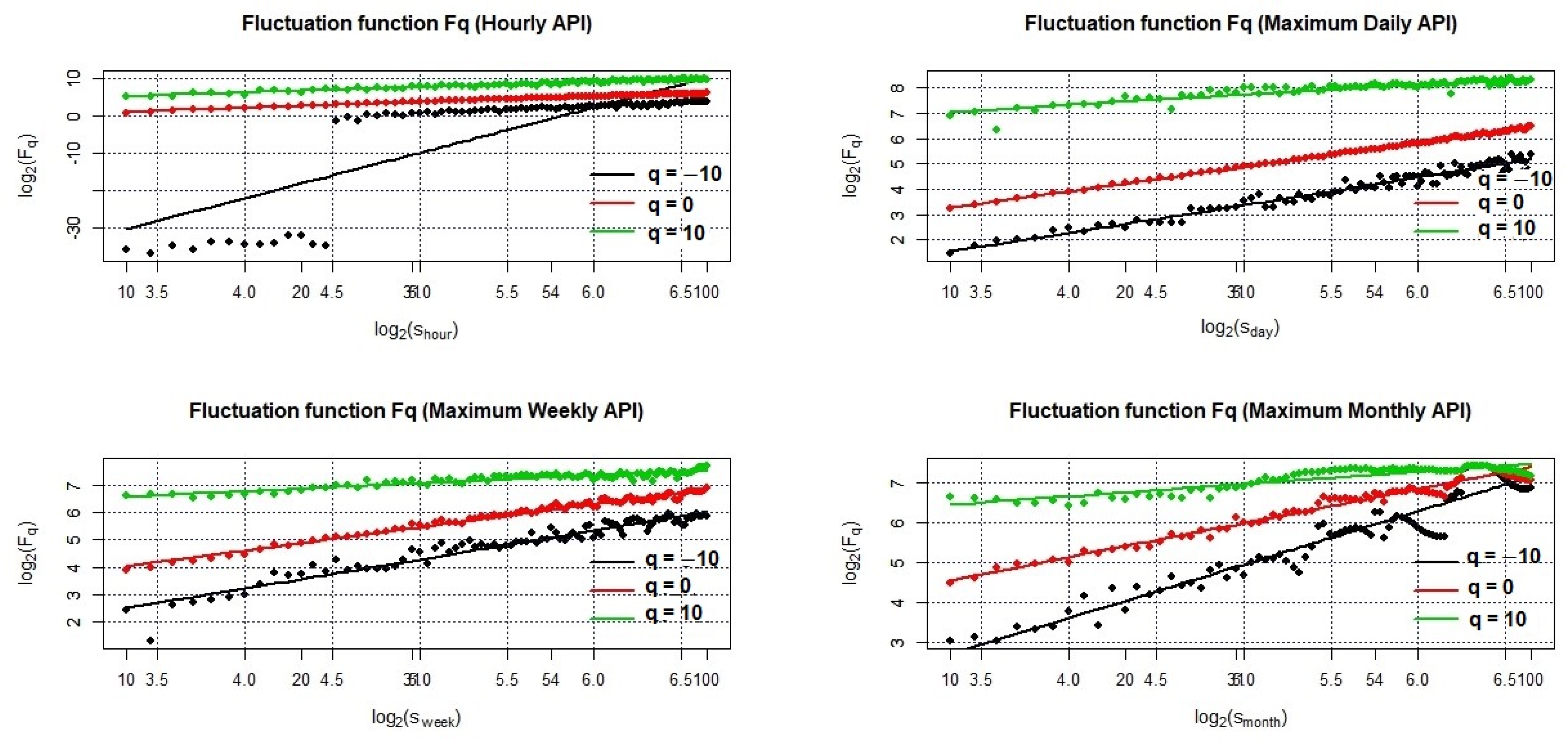
Figure 4 shows the properties of linear relationships in the plots of ln(s) versus ln(Fq(s)) for all q moments of different durations of maximum air pollution series, except for hourly API with moment q = −10. The results imply the existence of power-law relationships. In fact, as described above, the linear behavior on the logarithmic scale for moments q = −10, 0, and 10 indicate the multifractal behaviors of the air pollution series. In addition, as reported by Dong et al. [63], converging regression lines for different orders of q indicate the multifractal nature of the original series. Similarly, Weerasinghe et al. [64] reported that parallel regression lines indicate a monofractal series and that, by contrast, non-parallel regression lines indicate a multifractal series. In Figure 4, a series of maximum daily, weekly, and monthly APIs clearly show a significant convergence of fluctuation functions for different orders of q. These results provide a preliminary assumption about multifractal behavior. However, the series of hourly API indicates parallel properties between moments of q = 0 and q = 10, while the linear relationship fails to represent the plots of ln(s) versus ln(Fq(s)) at the moment of q = −10. This scenario is difficult to interpret as it shows no clear pattern for multifractality.
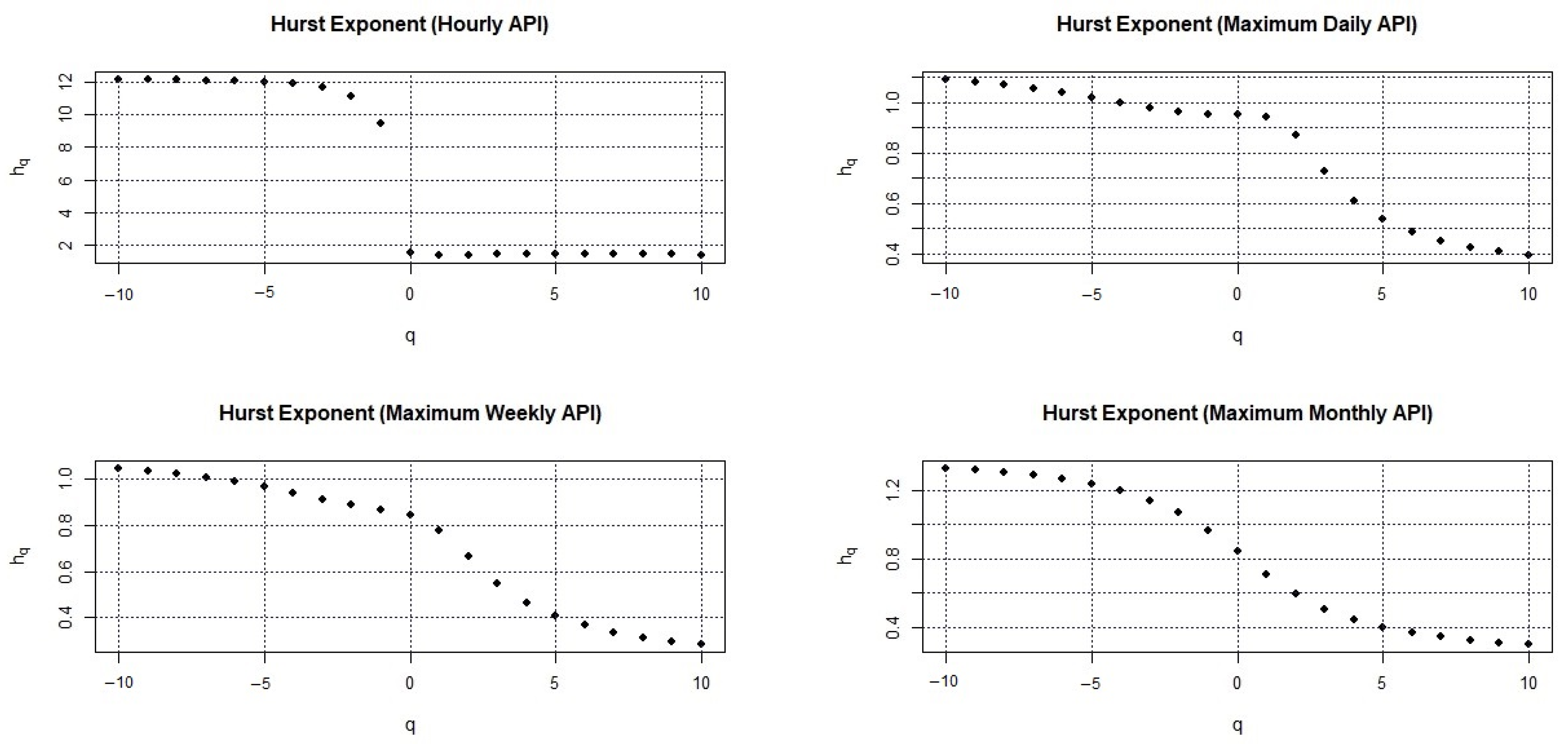
Further investigation is carried out by analyzing the plots of Rényi/Mass exponents. Figure 5 shows the nonlinear relationships for the hourly air pollution indices series in Klang. As reported by da Silva et al. [56], the Rényi exponent provides information about the relationships among τ(q) functions for different orders of q. Nonlinear relationships imply characteristics of multifractal processes. In Figure 5, the maximum API series for all durations indicates nonlinear relationships between the τ(q) function and their q-moment values. Thus, multifractal properties may exist on maximum API series regardless of their different durations. The same argument can be applied on the plots of Hurst exponents in this study. Figure 6 clearly shows the generalized Hurst exponent plots where the h(q) functions are nonlinearly dependent on q; their functions decrease when the value of q increases for all series of maximum APIs. As described by Miloş et al. [65], the decreasing function presented by generalized the Hurst exponent reveals the presence of multifractal behaviors. The results of Figure 5 and Figure 6 are thus in an agreement.
In addition, h(q) values that are larger than 0.5 indicate that the series may have properties of long memory, with persistent large and small fluctuations. In parallel, as previously described by Shi [66], the series also indicates nonstationary signals with a long-range power-law correlation. By comparison, h(q) values less than 0.5 indicate that the air pollution series may have short-term memory, with intermittent or non-persistent behaviors in both large and small fluctuations. Furthermore, h(q) values equal to 0.5 indicate complete random behaviors of the air pollution series. Figure 7a shows the values of Δ h ( q ) for API series with different durations in Klang. Clearly, the Δ h ( q ) value for the hourly API series is greater than those of any other duration, indicating that the variation in the distribution of fluctuations for hourly air pollution indices is greater than those determined by daily, weekly, or monthly series. In terms of air pollution behaviors, the results also imply that the information provided by the hourly API series indicate the heterogeneity and complexity of the temporal distribution while the other duration series represent homogeneous and regular temporal distributions.
Apart from that, the generalized Hurst exponent plots in Figure 6 clearly show that the h(q) function is nonlinearly dependent on q; these functions decrease when the values of q increase for all durations of the maximum API series. In addition, the changes of h(q) also provide information regarding the dependency of the variation of small fluctuations if q < 0 and depend mainly on the variation of large fluctuations if q > 0. Figure 7b shows that the Δ h q < 0 value is larger than Δ h q > 0 for the hourly API series. Thus, the information provided by the hourly pollution series is highly influenced by the variations from small fluctuations. This implies that the hourly API series are densely clustered in time domains almost the same as the sparsely populated domains. By contrast, for the daily, weekly, or monthly API series, the reverse scenario occurs. Their Δ h q < 0 values are slightly smaller or almost have the same magnitude with Δ h q > 0 . This result indicates that their variation can be influenced by large fluctuations of air pollution. Thus, the hourly pollution series presents densely clustered time domains that are more heterogeneous and complex than the information based on daily, weekly, or monthly series.
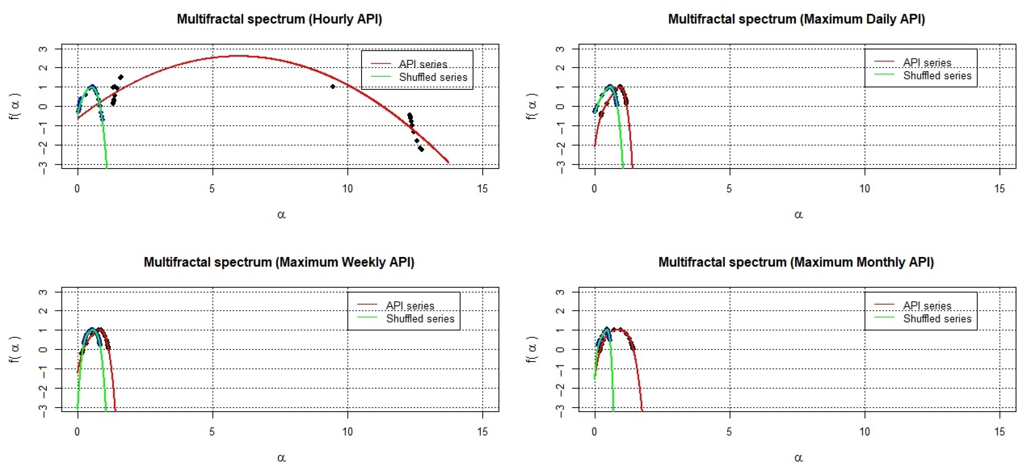
Another perfective that can be explored is the multifractal features of air pollution series that can be determined using the concept of the singularity spectrum. Figure 8 shows the singularity spectrum f ( α ) plots on each maximum API series corresponding to their Hölder exponent α . The spectrum for all the plots is not constant over all α values and, thus, all series do not indicate monofractal characteristics. These results provide a similar conclusion with the plots of Rényi and the generalized Hurst exponents. In fact, the shape of f ( α ) confirms that the temporal dynamics of the air pollution series belong to multifractal processes with a fourth-degree polynomial to represent the singularity spectra that determine the complexity measures. These results provide an agreement with results presented by several researchers regarding the multifractal characteristics of air pollution behaviors [30,63,67]. Thus, the complexity parameters can determine a singularity spectrum on each different API series. Table 2 presents the multifractal parameters of the air pollution series in Klang. The parameter α 0 represents the position of maxima in the singularity spectrum. The API series with values of the exponent α 0 greater than 0.5 indicate fluctuations with persistent long-term correlations, as shown by the information provided by the hourly API series. This result means that the information on persistent long-term correlations on the air pollution series is lost if the data are represented daily, weekly, or monthly.
Moreover, the value of Δ α = α max α min represent the spectrum width that determines the strength of the multifractality present in the series. This value can be estimated by extrapolating the fitted polynomial to f ( α max ) = f ( α min ) = 0 . The hourly API series has the greatest strength of multifractality, followed by the monthly, weekly, and daily series. Meanwhile, the asymmetry parameter index R represents the degree of skewness of the spectrum, where the value R = 0 indicates symmetry. R > 0 indicates properties of a left-skewed spectrum that implies the dominance of high fluctuations, such as in the daily, weekly, and monthly API data. R < 0 indicates a right-skewed spectrum that implies the dominance of low fluctuations, as seen in the hourly API series.
The multifractality behaviors described above are possibly influenced by two types of sources, namely, different long-range temporal correlations for small and large fluctuations as well as a fat-tailed probability distribution of variations [68]. With the aim of investigating the main sources of multifractality in the API data in Klang, the original series are shuffled to remove any temporal correlations caused by long- or short-term memories in data. However, the shuffled data retain exactly the same fluctuation distributions, meaning they provide similar behaviors to random walk processes but present weak multifractal properties. In Figure 8, the range of change of f ( α ) for the hourly API series decreases significantly after the reshuffling of the original series. This result implies a reduction in terms of the degree of multifractality, where shuffling the series moves the spectrum to the left. This scenario concludes that the multifractality behaviors for the hourly API series are caused by long-term correlations. Thus, the implication is that a nonlinear temporal correlation is the major contributor in multifractality formation. In fact, the significantly narrowed widths of spectra conclude that the multifractality is also influenced by non-normal distribution. However, for other API series, the change of spectra for both the original and shuffled series show no significant difference. Thus, the multifractality behaviors in these series are already weak. Neither nonlinear temporal correlation nor fat-tail distribution highly influence the daily, weekly, or monthly API data.

6. Conclusions

This study investigates multifractality properties on the series of maximum API in Malaysia in different durations, namely hourly, daily, weekly, and monthly. The Multifractal Detrended Fluctuation Analysis (MFDFA) is adopted to evaluate the fluctuations of the maximum API series in terms of partition intervals as statistical points. On this basis, a generalized Hurst exponent is determined to represent the power-law property of the fluctuation function, evaluate the fluctuation singularity, and provide information on the complexity and persistence of the API series. The MFDFA technique is found to have advantages in examining a higher-dimensional fractal and multifractal characteristics hidden in an air pollution series. The results show that only the hourly API series exhibit persistent long-term correlations as determined by a Hurst exponent value greater than 0.5. In addition, this series also exhibits multifractality behaviors with a dominance of small fluctuations. The other durations of the maximum API series (daily, weekly, and monthly) show weak multifractality behaviors, indicating that the hourly API series contain the most informative data regarding the behaviors and characteristic of air pollution events.
To summarize, this study contributes to knowledge related to multifractal behavior changes in air pollution data series that undergo a data reduction process. In particular, a data reduction corresponds to a longer time length and implies several consequences, namely: (i) it changes the properties of the heterogeneity and complexity of the temporal distribution to be more homogeneous with regular temporal distributions; (ii) the variation of the series will be change from being densely clustered in time domains into variations that are influenced by large fluctuations; (iii) the strength of the multifractality in the series will be weakened; and (iv) the information about the persistent and long-term correlations on the original series will also be lost. However, the MFDFA method is bound by some limitations. The is MFDFA not able to reveal the asymmetric properties of multifractal scaling behaviors that might exist in the air pollution series data. Thus, for future research, this study recommends the adaption of asymmetric multifractal detrended fluctuation analysis to overcome this issue.
Overall, this study contributes to a better understanding of the stochastic processes that generate air quality variability in Malaysia. The findings can help in better understanding the mechanisms governing the dynamics of air pollution series and in performing better air quality assessments.

Funding

This research and the APC fees were funded by UNIVERSITI KEBANGSAAN MALAYSIA, grant number GP-2021-K020446 and PP-FST-2022.

Institutional Review Board Statement

Not applicable.

Informed Consent Statement

Not applicable.

Data Availability Statement

Due to confidentiality agreements, supporting data can only be made available to bona fide researchers subject to a non-disclosure agreement. Details of the data and how to request access are available from https://www.doe.gov.my/portalv1/en/at (accessed on 4 June 2022). Department of Environment Malaysia.

Acknowledgments

The authors are indebted Malaysian Department of Environment for providing air pollution data.

Conflicts of Interest

The authors declare no conflict of interest.

Abbreviations

The following abbreviations are used in this manuscript:
Nomenclature
R Asymmetry index
a ^ i Estimated polynomial coefficient
h ( q ) Generalized Hurst exponent
y ¯ Mean of the series
Y v ( i ) m-th polynomial order in segment v
N s Non-overlapping segments with a length s
y ( t ) Observed data
F q ( s ) q-order fluctuation function
τ ( q ) Rényi exponent
Y ( i ) Signal profile series
f ( α ) Singularity spectrum
F 2 ( s , v ) Variance for segment v
Greek symbols
α Lipschitz–Hölder exponent
α 0 Maxima position in the singularity spectrum
α max Maximum value of the Hölder exponent
α min Minimum value of the Hölder exponent
Δ α L Left-hand branch of the singularity spectrum curve
Δ α R Right-hand branch of the singularity spectrum curve
Δ α Spectrum width
Acronyms
APIAir pollution index
COCarbon monoxide
MFDFAMultifractal detrended fluctuation analysis
NO2Nitrogen dioxide
O3Ozone
SO2Sulfur dioxide
PM10Suspended particulate matter with size less than 10 microns
Subscripts
sLength of segment
qFluctuation order
Superscript
vSegment of the series
mPolynomial order

References

  1. Bhat, T.H.; Jiawen, G.; Farzaneh, H. Air Pollution Health Risk Assessment (AP-HRA), Principles and Applications. Int. J. Environ. Res. Public Health 2021, 18, 1935. [Google Scholar] [CrossRef] [PubMed]
  2. Chen, F.; Chen, Z. Cost of economic growth: Air pollution and health expenditure. Sci. Total Environ. 2021, 755, 142543. [Google Scholar] [CrossRef] [PubMed]
  3. Chen, Y.; Xu, Y.; Wang, F. Air pollution effects of industrial transformation in the Yangtze River Delta from the perspective of spatial spillover. J. Geogr. Sci. 2022, 32, 156–176. [Google Scholar] [CrossRef]
  4. Zeng, J.; Wen, Y.; Bi, C.; Feiock, R. Effect of tourism development on urban air pollution in China: The moderating role of tourism infrastructure. J. Clean. Prod. 2021, 280, 124397. [Google Scholar] [CrossRef]
  5. Lin, Y.; Huang, R.; Yao, X. Air pollution and environmental information disclosure: An empirical study based on heavy polluting industries. J. Clean. Prod. 2021, 278, 124313. [Google Scholar] [CrossRef]
  6. Cariolet, J.-M.; Colombert, M.; Vuillet, M.; Diab, Y. Assessing the resilience of urban areas to traffic-related air pollution: Application in Greater Paris. Sci. Total Environ. 2018, 615, 588–596. [Google Scholar] [CrossRef]
  7. Yang, J.; Shi, B.; Shi, Y.; Marvin, S.; Zheng, Y.; Xia, G. Air pollution dispersal in high density urban areas: Research on the triadic relation of wind, air pollution, and urban form. Sustain. Cities Soc. 2020, 54, 101941. [Google Scholar] [CrossRef]
  8. Afroz, R.; Hassan, M.N.; Ibrahim, N.A. Review of air pollution and health impacts in Malaysia. Environ. Res. 2003, 92, 71–77. [Google Scholar] [CrossRef]
  9. Gocheva-Ilieva, S.G.; Ivanov, A.V.; Voynikova, D.S.; Boyadzhiev, D.T. Time series analysis and forecasting for air pollution in small urban area: An SARIMA and factor analysis approach. Stoch. Environ. Res. Risk Assess. 2014, 28, 1045–1060. [Google Scholar] [CrossRef]
  10. Masseran, N. Modeling fluctuation of PM10 data with existence of volatility effect. Environ. Eng. Sci. 2017, 34, 816–827. [Google Scholar] [CrossRef]
  11. Masseran, N.; Hussain, S.I. Copula modelling on the dynamic dependence structure of multiple air pollutant variables. Mathematics 2020, 8, 1910. [Google Scholar] [CrossRef]
  12. Liu, H.; Yan, G.; Duan, Z.; Chen, C. Intelligent modeling strategies for forecasting air quality time series: A review. Appl. Soft Comput. 2021, 102, 106957. [Google Scholar] [CrossRef]
  13. Ravindra, K.; Rattan, P.; Mor, S.; Aggarwal, A.N. Generalized additive models: Building evidence of air pollution, climate change and human health. Environ. Int. 2019, 132, 104987. [Google Scholar] [CrossRef] [PubMed]
  14. Roca-Pardiñas, J.; Ordóñez, C. Predicting pollution incidents through semiparametric quantile regression models. Stoch. Environ. Res. Risk Assess. 2019, 33, 673–685. [Google Scholar] [CrossRef]
  15. Masseran, N. Modeling the characteristics of unhealthy air pollution events: A copula approach. Int. J. Environ. Res. Public Health 2021, 18, 8751. [Google Scholar] [CrossRef] [PubMed]
  16. Álvarez-Liébana, J.; Ruiz-Medina, M.D. Prediction of air pollutants PM10 by ARBX(1) processes. Stoch. Environ. Res. Risk Assess. 2019, 33, 1721–1736. [Google Scholar] [CrossRef]
  17. Huang, C.; Zhao, X.; Cheng, W.; Ji, Q.; Duan, Q.; Han, Y. Statistical Inference of dynamic conditional Generalized Pareto Distribution with weather and air quality factors. Mathematics 2022, 10, 1433. [Google Scholar] [CrossRef]
  18. Jiang, P.; Li, C.; Li, R.; Yang, H. An innovative hybrid air pollution early-warning system based on pollutants forecasting and Extenics evaluation. Knowl. Based. Syst. 2019, 164, 174–192. [Google Scholar] [CrossRef]
  19. Masseran, N. Power-law behaviors of the duration size of unhealthy air pollution events. Stoch. Environ. Res. Risk Assess. 2021, 35, 1499–1508. [Google Scholar] [CrossRef]
  20. Zhou, Y.; Chang, F.-J.; Chang, L.-C.; Kao, I.-F.; Wang, Y.-S. Explore a deep learning multi-output neural network for regional multi-step-ahead air quality forecasts. J. Clean. Prod. 2019, 209, 134–145. [Google Scholar] [CrossRef]
  21. Al-Janabi, S.; Mohammad, M.; Al-Sultan, A. A new method for prediction of air pollution based on intelligent computation. Soft Comput. 2020, 24, 661–680. [Google Scholar] [CrossRef]
  22. Sayeed, A.; Choi, Y.; Eslami, E.; Lops, Y.; Roy, A.; Jung, J. Using a deep convolutional neural network to predict 2017 ozone concentrations, 24 hours in advance. Neural Netw. 2020, 121, 396–408. [Google Scholar] [CrossRef]
  23. Saez, M.; Barceló, M.A. Spatial prediction of air pollution levels using a hierarchical Bayesian spatiotemporal model in Catalonia, Spain. Environ. Model. Softw. 2002, 151, 105369. [Google Scholar] [CrossRef]
  24. Ding, W.; Leung, Y.; Zhang, J.; Fung, T. A hierarchical Bayesian model for the analysis of space-time air pollutant concentrations and an application to air pollution analysis in Northern China. Stoch. Environ. Res. Risk Assess. 2021, 35, 2237–2271. [Google Scholar] [CrossRef]
  25. Liu, C.-C.; Lin, T.-C.; Yuan, K.-Y.; Chiueh, P.-T. Spatio-temporal prediction and factor identification of urban air quality using support vector machine. Urban Clim. 2022, 41, 101055. [Google Scholar] [CrossRef]
  26. Gyarmati-Szabó, J.; Bogachev, L.V.; Chen, H. Nonstationary POT modelling of air pollution concentrations: Statistical analysis of the traffic and meteorological impact. Environmetrics 2017, 28, e2449. [Google Scholar] [CrossRef] [Green Version]
  27. Masseran, N.; Mohd Safari, M.A. Intensity–duration–frequency approach for risk assessment of air pollution events. J. Environ. Manag. 2020, 264, 110429. [Google Scholar] [CrossRef]
  28. Vettori, S.; Huser, R.; Genton, M.G. Bayesian modeling of air pollution extremes using nested multivariate max-stable processes. Biometrics 2019, 75, 831–841. [Google Scholar] [CrossRef]
  29. Yadav, M.; Singh, N.K.; Sahu, S.P.; Padhiyar, H. Investigations on air quality of a critically polluted industrial city using multivariate statistical methods: Way forward for future sustainability. Chemosphere 2022, 291, 133024. [Google Scholar] [CrossRef]
  30. Wang, Q. Multifractal characterization of air polluted time series in China. Phys. A Stat. Mech. Appl. 2019, 514, 167–180. [Google Scholar] [CrossRef]
  31. Li, X. On the multifractal analysis of air quality index time series before and during COVID-19 partial lockdown: A case study of Shanghai, China. Phys. A Stat. Mech. Appl. 2021, 565, 125551. [Google Scholar] [CrossRef] [PubMed]
  32. Frenzel, S.; Pompe, B. Partial mutual information for coupling analysis of multivariate time series. Phys. Rev. Lett. 2007, 99, 204101. [Google Scholar] [CrossRef] [PubMed]
  33. Jauregui, M.; Zunino, L.; Lenzi, E.K.; Mendes, R.S.; Ribeiro, H.V. Characterization of time series via Rényi complexity–entropy curves. Phys. A Stat. Mech. Appl. 2018, 498, 74–85. [Google Scholar] [CrossRef] [Green Version]
  34. Kantelhardt, J.W.; Zschiegner, S.A.; Koscielny-Bunde, E.; Havlin, S.; Bunde, A.; Stanley, H.E. Multifractal detrended fluctuation analysis of nonstationary time series. Phys. A Stat. Mech. Appl. 2002, 316, 87–114. [Google Scholar] [CrossRef] [Green Version]
  35. Carrizales-Velazquez, C.; Donner, R.V.; Guzmán-Vargas, L. Generalization of Higuchi’s fractal dimension for multifractal analysis of time series with limited length. Nonlinear Dyn. 2022, 108, 417–431. [Google Scholar] [CrossRef]
  36. Jiang, P.; Wang, B.; Li, H.; Lu, H. Modeling for chaotic time series based on linear and nonlinear framework: Application to wind speed forecasting. Energy 2019, 173, 468–482. [Google Scholar] [CrossRef]
  37. Zou, Y.; Donner, R.V.; Marwan, N.; Donges, J.F.; Kurths, J. Complex network approaches to nonlinear time series analysis. Phys. Rep. 2019, 787, 1–97. [Google Scholar] [CrossRef]
  38. Chen-hua, S.; Yi, H.; Ya-ni, Y. An analysis of multifractal characteristics of API time series in Nanjing, China. Phys. A Stat. Mech. Appl. 2016, 451, 171–179. [Google Scholar]
  39. Liu, Z.; Wang, L.; Zhu, H. A time–scaling property of air pollution indices: A case study of Shanghai, China. Atmos. Pollut. Res. 2015, 6, 886–892. [Google Scholar] [CrossRef]
  40. Xu, W.; Liu, C.; Shi, K.; Liu, Y. Multifractal detrended cross-correlation analysis on NO, NO2 and O3 concentrations at traffic sites. Phys. A Stat. Mech. Appl. 2018, 502, 605–612. [Google Scholar] [CrossRef]
  41. Manimaran, P.; Narayana, A.C. Multifractal detrended cross-correlation analysis on air pollutants of University of Hyderabad Campus, India. Phys. A Stat. Mech. Appl. 2018, 502, 228–235. [Google Scholar] [CrossRef]
  42. Cárdenas-Moreno, P.R.; Moreno-Torres, L.R.; Lovallo, M.; Telesca, L.; Ramírez-Rojas, A. Spectral, multifractal and informational analysis of PM10 time series measured in Mexico City Metropolitan Area. Phys. A Stat. Mech. Appl. 2021, 565, 125545. [Google Scholar] [CrossRef]
  43. Masseran, N. Multifractal characteristics on multiple pollution variables in Malaysia. Bull. Malays. Math. Sci. Soc. 2022, 45, 325–344. [Google Scholar] [CrossRef]
  44. Plocoste, T.; Pavón-Domínguez, P. Temporal scaling study of particulate matter (PM10) and solar radiation influences on air temperature in the Caribbean basin using a 3D joint multifractal analysis. Atmos. Environ. 2020, 222, 117115. [Google Scholar] [CrossRef]
  45. Wang, J.; Shao, W.; Kim, J. Multifractal detrended cross-correlation analysis between respiratory diseases and haze in South Korea. Chaos Solitons Fractals 2020, 135, 109781. [Google Scholar] [CrossRef]
  46. Wang, J.; Kim, J.; Shao, W. Investigation of the implications of “Haze Special Law” on air quality in South Korea. Complexity 2020, 2022, 6193016. [Google Scholar] [CrossRef] [Green Version]
  47. Zhang, C.; Ni, Z.; Ni, L. Multifractal detrended cross-correlation analysis between PM2.5 and meteorological factors. Phys. A Stat. Mech. Appl. 2015, 438, 114–123. [Google Scholar] [CrossRef]
  48. Gin, O.K. Historical Dictionary of Malaysia; Scarecrow Press: Lanham, MD, USA, 2009; pp. 157–158. [Google Scholar]
  49. Masseran, N.; Safari, M.A.M. Risk assessment of extreme air pollution based on partial duration series: IDF approach. Stoch. Environ. Res. Risk Assess. 2020, 34, 545–559. [Google Scholar] [CrossRef]
  50. Google. 2019. Available online: https://maps.googleapis.com/maps/api/geocode/json?address=Klang%2CSelangor&key=xxx (accessed on 13 April 2022).
  51. Department of Environment. A Guide to Air Pollutant Index in Malaysia (API); Ministry of Science, Technology and the Environment: Kuala Lumpur, Malaysia, 1997. Available online: https://aqicn.org/images/aqi-scales/malaysia-api-guide.pdf (accessed on 13 February 2022).
  52. Masseran, N.; Safari, M.A.M. Mixed POT-BM approach for modeling unhealthy air pollution events. Int. J. Environ. Res. Public Health 2021, 18, 6754. [Google Scholar] [CrossRef]
  53. Masseran, N. Power-law behaviors of the severity levels of unhealthy air pollution events. Nat. Hazards 2022, 112, 1749–1766. [Google Scholar] [CrossRef]
  54. Cao, G.; He, L.-Y.; Cao, J. Multifractal Detrended Analysis Method and Its Application in Financial Markets; Springer: Singapore, 2018. [Google Scholar]
  55. Hou, W.; Feng, G.; Yan, P.; Li, S. Multifractal analysis of the drought area in seven large regions of China from 1961 to 2012. Meteorol. Atmos. Phys. 2018, 130, 459–471. [Google Scholar] [CrossRef]
  56. da Silva, H.S.; Silva, J.R.S.; Stosic, T. Multifractal analysis of air temperature in Brazil. Phys. A Stat. Mech. Appl. 2020, 549, 124333. [Google Scholar] [CrossRef]
  57. Chattopadhyay, A.; Khondekar, M.H.; Bhattacharjee, A.R. Fractality and singularity in CME linear speed signal: Cycle 23. Chaos Solit. Fractals 2018, 114, 542–550. [Google Scholar] [CrossRef]
  58. Mali, P.; Manna, S.K.; Mukhopadhyay, A.; Haldar, P.K.; Singh, G. Multifractal analysis of multiparticle emission data in the framework of visibility graph and sandbox algorithm. Phys. A Stat. Mech. Appl. 2018, 493, 253–266. [Google Scholar] [CrossRef]
  59. Sun, Y.; Yuan, X. Nonlinear relationship between money market rate and stock market liquidity in China: A multifractal analysis. PLoS ONE 2021, 16, e0249852. [Google Scholar] [CrossRef] [PubMed]
  60. Wu, W.; Yuan, N.; Xie, F.; Qi, Y. Understanding long-term persistence and multifractal behaviors in river runoff: A detailed study over eastern China. Phys. A Stat. Mech. Appl. 2019, 533, 122042. [Google Scholar] [CrossRef]
  61. Adarsh, S.; Nourani, V.; Archana, D.S.; Dharan, D.S. Multifractal description of daily rainfall fields over India. J. Hydrol. 2020, 586, 124913. [Google Scholar] [CrossRef]
  62. Xie, S.; Bao, Z. Fractal and multifractal properties of geochemical fields. Math. Geol. 2004, 36, 847–864. [Google Scholar] [CrossRef]
  63. Dong, Q.; Wang, Y.; Li, P. Multifractal behavior of an air pollutant time series and the relevance to the predictability. Environ. Pollut. 2017, 222, 444–457. [Google Scholar] [CrossRef]
  64. Weerasinghe, R.M.; Pannila, A.S.; Jayananda, M.K.; Sonnadara, D.U.J. Multifractal behavior of wind speed and wind direction. Fractals 2016, 24, 1650003. [Google Scholar] [CrossRef]
  65. Miloş, L.R.; Haţiegan, C.; Miloş, M.C.; Barna, F.M.; Boțoc, C. Multifractal detrended fluctuation analysis (MF-DFA) of stock market indexes. Empirical evidence from seven central and Eastern European markets. Sustainability 2020, 12, 535. [Google Scholar] [CrossRef]
  66. Shi, K. Multifractal processes and self-organized criticality of PM2.5 during a typical haze period in chengdu, China. Aerosol Air Qual. Res. 2015, 15, 926–934. [Google Scholar] [CrossRef] [Green Version]
  67. Xue, Y.; Pan, W.; Lu, W.-Z.; He, H.-D. Multifractal nature of particulate matters (PMs) in Hong Kong urban air. Sci. Total Environ. 2015, 532, 744–751. [Google Scholar] [CrossRef] [PubMed]
  68. Kwapien, J.; Oswiecimka, P.; Drozdz, S. Components of multifractality in high-frequency stock returns. Phys. A Stat. Mech. Appl. 2005, 350, 466–474. [Google Scholar] [CrossRef]
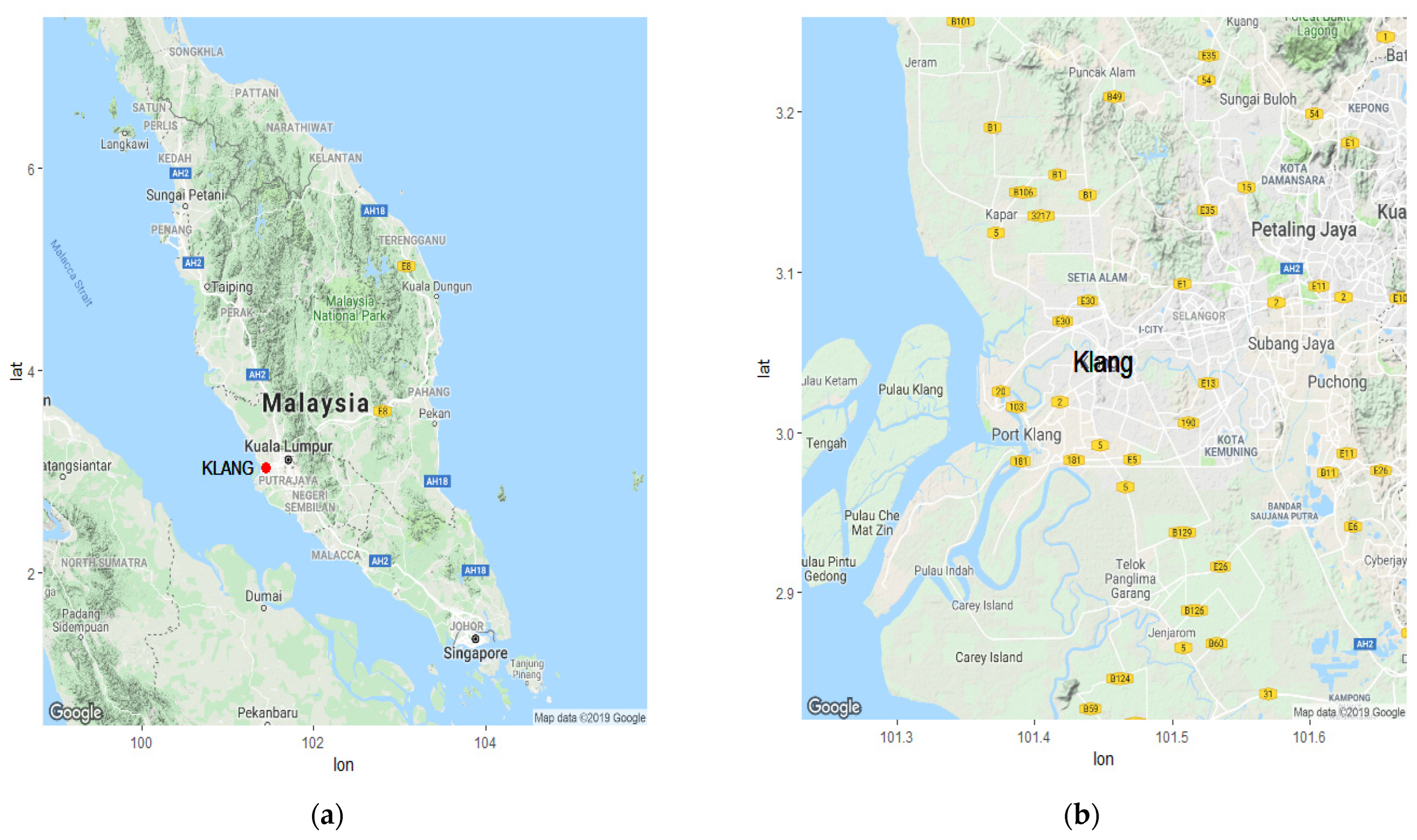
Figure 1. (a) Map of Peninsular Malaysia with Klang identified by a red dot, (b) Map of Klang [50].
Mathematics 10 03910 g001
Figure 2. Process of determining the API value [53].
Mathematics 10 03910 g002
Figure 3. Time series plots of maximum API for different time lengths.
Mathematics 10 03910 g003
Figure 4. Plots of ln(s) versus ln(Fq(s)) on maximum air pollution indices series in Klang.
Mathematics 10 03910 g004
Figure 5. Nonlinear relationships between τ(q) and q for hourly API series in Klang.
Mathematics 10 03910 g005
Figure 6. Plots of h(q) versus q for hourly API series in Klang.
Mathematics 10 03910 g006
Figure 7. (a) Δ h ( q ) values for API series with different durations in Klang, (b) sectional Δ h ( q ) .
Mathematics 10 03910 g007
Figure 8. Multifractal spectrum plots.
Mathematics 10 03910 g008
Table 1. Statistical characteristics of API data for different time lengths.
VariableMeanVarianceMin.Max.MedianSkewnessKurtosis
Hourly API55.735434.4480543544.73868.370
Max. Daily API65.530548.75821543615.56174.658
Max. Weekly API83.3821129.1240543765.60855.403
Max. Monthly API105.8612444.43160543934.77933.222
Table 2. Multifractal parameters air pollution series in Klang.
Duration α min α max α 0 Δ α L Δ α R Δ α R Δ f ( α )
Hourly1.32212.7461.5110.18911.23511.424−0.967−3.779
Daily0.2371.1800.9520.7150.2280.9430.516−1.490
Weekly0.1571.1440.8430.6860.3010.9880.390−1.254
Monthly0.1900.2590.8440.6540.5851.2390.056−1.107
Publisher’s Note: MDPI stays neutral with regard to jurisdictional claims in published maps and institutional affiliations.