Some Technical Remarks on Negations of Discrete Probability Distributions and Their Information Loss

Abstract

Negation of a discrete probability distribution was introduced by Yager. To date, several papers have been published discussing generalizations, properties, and applications of negation. The recent work by Wu et al. gives an excellent overview of the literature and the motivation to deal with negation. Our paper focuses on some technical aspects of negation transformations. First, we prove that independent negations must be affine-linear. This fact was established by Batyrshin et al. as an open problem. Secondly, we show that repeated application of independent negations leads to a progressive loss of information (called monotonicity). In contrast to the literature, we try to obtain results not only for special but also for the general class of $\varphi$-entropies. In this general framework, we can show that results need to be proven only for Yager negation and can be transferred to the entire class of independent (=affine-linear) negations. For general $\varphi$-entropies with strictly concave generator function $\varphi$, we can show that the information loss increases separately for sequences of odd and even numbers of repetitions. By using a Lagrangian approach, this result can be extended, in the neighbourhood of the uniform distribution, to all numbers of repetition. For Gini, Shannon, Havrda–Charvát (Tsallis), Rényi and Sharma–Mittal entropy, we prove that the information loss has a global minimum of 0. For dependent negations, it is not easy to obtain analytical results. Therefore, we simulate the entropy distribution and show how different repeated negations affect Gini and Shannon entropy. The simulation approach has the advantage that the entire simplex of discrete probability vectors can be considered at once, rather than just arbitrarily selected probability vectors.

1. Introduction

In knowledge-based systems, terms with n categories can be characterized by probability distributions. Let us consider the term ”conservative” and assume that we know how the conservative population is distributed among the three categories ”right-wing conservative”, ”conservative” and ”liberal-conservative”. Can we learn anything about the non-conservative population from this distribution by looking at the negation of the original distribution? If so, does this not necessarily involve a loss of information, because the original distribution makes no explicit statement about non-conservatism? Can the loss of information be measured by any information measure? These are questions that are still the subject of intense debate that starts with the seminal work of Yager [1]. He proposed to define negation of a probability distribution by subtracting the probability distribution from 1 and distributing the sum of negated probabilities equally among the n categories. The equal distribution can be motivated by Dempster–Shafer theory and a maximal entropy argument. Technically, the equal distribution means that the negation of one category’s probability must not depend on the probabilities of the other categories. Batyrshin et al. [2] call a negation with this property ”independent”. Yager negation and all other affine-linear negations are independent. Batyrshin [3] stated this as an open problem to show that independent negations must be affine-linear. One of our technical remarks concerns the solution of this open problem.

In particular, for Yager negation, information content and information loss have been measured by different entropies. Yager [1] discussed Gini entropy. This entropy is very popular because no complicated calculations are required. However, the question arises whether the results obtained for Gini entropy can be transferred to other entropies. Therefore, Gao and Deng [4,5] have considered Shannon and Havrda–Charvát entropy. Zhang et al. [6] also studied Havrda–Charvát entropy and Wu et al. [7] Shannon entropy for exponential negations. Srivastava and Maheswari [8] introduced a new kind of entropy tailored for Yager negation. Their proposal is also based on Shannon entropy. All authors concluded that negation leads to an information loss. They use a Lagrangian approach to reach this conclusion. Because the articles mentioned mostly deal with the application of negations in various scientific fields, the more technical aspects seem to be of less interest. In particular, the sufficient conditions for optimization have not been investigated. Therefore, our technical remarks are intended to complete the proofs and generalise the results to the class of $\varphi$-entropies with strictly concave generating function $\varphi$.

Negations can be applied not only to the original probability vector, but also to the negation of a probability vector because negation again gives a probability distribution. For example, consider a sequence of recursive application of negation of length $k+1$. Then, Yager [1] showed for Yager negation and Batyrshin et al. [3] proved for general affine-linear negations that the $k+1$-times recursively applied negation is given by a recursion relation that updates the k-times recursively repeated negation by the uniform distribution. Convergence against the uniform distribution with $k\to \infty$ is easy to show. We ask whether this updating rule also applies to entropy of negation. In the tradition of Yager’s work, we focus on Gini entropy as the preferred information measure. We show that Gini entropy of $k+1$-times repeated independent negations is a convex combination of the Gini entropy of the uniform distribution and the Gini entropy of the k-times recursively repeated negations. It is well known that the uniform distribution maximises the Gini entropy and represents the point of minimum information, maximum dispersion, or maximum uncertainty. Therefore, this updating formula ensures that negation leads to an information loss as suspected in the introductory discussion of “conservatism”.

The work of Gao and Deng [4,5], Zhang et al. [6] and Wu et al. [7] illustrates the entropy behaviour in terms of negation by numerical examples. Typical probability vectors were selected and Yager or exponential negation were applied to this vector. As an alternative, we propose a numerical procedure to compare $\varphi$-entropies for all possible probability vectors. The numerical way is to draw probability vectors of size n from the Dirichlet distribution and to simulate the entropy distribution. This procedure is particularly recommended for dependent negations. In our opinion, there seems to be no analytical way to discuss the behaviour of dependent negations and the corresponding $\varphi$-entropies. For all negations considered, the entropy distribution is more or less concentrated below the entropy’s maximum value. What we can learn is that negations that lie above Yager negation (like exponential negation discussed in [7]) give more concentrated and peaked entropy distributions and negations that lie below the Yager negation (like the Tsallis negation with parameter $1/2$ [6]) give more spread and less peaked distributions. This confirms the statement of Wu et al. [7] that recursively repeated exponential negations converge faster to the uniform distribution than recursively repeated Yager negations.

The specific aims of our paper are as follows.

• It will be proven that independent negations have to be affine-linear.
• It will be proven that the uniform distribution maximizes all $\varphi$-entropies with strictly concave generating function $\varphi$.
• It will be proven that the Yager negation minimizes any $\varphi$-entropy in the class of affine-linear negations, with the consequence that the information loss has to be discussed only for Yager negation.
• It will be proven that the information loss, measured by the difference of $\varphi$-entropies, increases separately for odd and even sequences of repetition numbers of Yager negation.
• It will be proven that the uniform distribution yields a local minimum of the information loss produced by the Yager negation for each $\varphi$-entropy.
• It will be proven that the uniform distribution yields the global minimum of the information loss produced by the Yager negation for Gini, paired Shannon, Shannon and Havrda–Charvát entropy.
• An explicit formula for Yager negation’s information loss in the case of the Gini entropy will be given.
• It will be shown that results concerning the information loss of Havrda–Charvát entropy can be transferred to Rényi and Sharma–Mittal entropies by using the concept of $(h,\varphi )$-entropies with h strictly increasing.
• An impression of how the information loss behaves for dependent negations when analytical results do not seem to be available will be given.

The paper is organised along the lines of the abovementioned objectives. After some definitions in the first section, we show in the second section that independent negations must be affine-linear. The third section introduces $\varphi$-entropies and shows that they are maximized for the uniform distribution. Moreover, the Yager negation will be identified as a minimum $\varphi$ entropy representation of the class of affine-linear negations. The remainder of the section discusses the information loss of Yager negation for general $\varphi$-entropies. Approaches based on the strict concavity of $\varphi$ as well as the Lagrangian approach will be considered. In the fourth section, we elaborate on the results concerning the information loss for some prominent $\varphi$-entropies. The impression could be given that all $\varphi$-entropies behave similarly with respect to a negation. Therefore, we present some examples of entropies wherein negations behave differently. In the fifth section, we discuss the information loss for $(h,\varphi )$-entropies with strictly increasing function h. In the sixth section, we present the results of a simulation study for the information loss of dependent negations. The seventh section summarizes the main results. Three proofs refer to the same bordered Hessian matrix. For this reason, this matrix is dealt with in Appendix A. Three proofs are moved out to Appendix B to improve the readability.

2. Definitions

Let

$${\mathbf{I}}_n=\left\{(p_1,\dots ,p_n)\in {[0,1]}^n\mid \sum _{i=1}^n{p}_i=1\right\}$$

(1)

be the probability simplex of size $n\ge 1$. It contains all discrete probability distributions with support of size n. A probability transformation maps a discrete probability distribution to a new discrete probability distribution with support of the same size.

Definition 1.

• A probability transformation $\mathbf{T}$ maps ${\mathbf{I}}_n$ into ${\mathbf{I}}_n$ such that

  $$\mathbf{T}(p_1,\dots ,p_n)=\left(T_1(p_1,\dots ,p_n),\dots ,T_n(p_1,\dots ,p_n)\right)$$

  (2)
  with $T_i(p_1,\dots ,p_n)\ge 0$, $i=1,2,\dots ,n$ and ${\sum }_{i=1}^n{T}_i(p_1,\dots ,p_n)=1$ for all $(p_1,\dots ,p_n)$$\in {\mathbf{I}}_n$.
• The probability transformation $\mathbf{T}$ is independent, if there exists a function $T:[0,1]\to [0,1]$ such that

  $$\mathbf{T}(p_1,\dots ,p_n)=\left(T\left(p_1\right),\dots ,T\left(p_n\right)\right)$$

  (3)
  for all $(p_1,\dots ,p_n)\in {\mathbf{I}}_n$.

For an independent transformation, the function $T_i$ depends exactly on the i-th component $p_i$ and not on the other probabilities $p_j$, $j\ne i$ for $j=1,2,\dots ,n$.

Three examples, to be discussed in detail later, are the exponential, the cosine, and the affine-linear transformation. The first two are not and the last is independent.

Example 1.

• In Wu et al. [7] an exponential probability transformation with

  $$T_i(p_1,\dots ,p_n)=\frac{e^{-p_i}}{{\sum }_{l=1}^n{e}^{-p_l}},i=1,2,\dots ,n$$

  (4)
  was considered.
• Another example could be the cosinus transformation

  $$T_i(p_1,\dots ,p_n)=\frac{1+cos\left(\pi p_i\right)}{n+{\sum }_{l=1}^{n}cos\left(\pi p_l\right)},i=1,2,\dots ,n.$$

  (5)
• Affine-linear probability transformations are given by

  $$T_i(p_1,\dots ,n)=\frac{a+b{p}_i}{na+b}=:T\left(p_i\right)$$

  (6)
  for a and b such that $0\le T\left(p_i\right)\le 1$, $i=1,2,\dots ,n$.

The transformations (4), (5) and the affine-linear transformation (6) with $b<0$ are negative transformations (called negations) in the following sense.

Definition 2.

• The probability transformation $\mathbf{N}:{\mathbf{I}}_n\to {\mathbf{I}}_n$ with

  $$\mathbf{N}(p_1,\dots ,p_n)=\left(N_1(p_1,\dots ,p_n),\dots ,N_n(p_1,\dots ,p_n)\right)$$
  is called a negation, if

  $$p_i\le p_j⟹N_i(p_1,\dots ,p_n)\ge N_j(p_1,\dots ,p_n)$$

  (7)
  for all $i,j=1,2,\dots ,n$ and $(p_1,\dots ,p_n)\in {\mathbf{I}}_n$.
• For independent negations $\mathbf{N}$ there exists a function $N:[0,1]\to [0,1]$ with

  $$\mathbf{N}(p_1,\dots ,p_n)=(N\left(p_1\right),\dots ,N\left(p_n\right)),(p_1,\dots ,p_n)\in {\mathbf{I}}_n.$$

  (8)
  N will be called a negator [3].

We will highlight two affine-linear negations that play a central role in what follows.

Example 2.

An affine-linear negator is given by

$$N\left(p\right)=\frac{a+bp}{na+b},0\le p\le 1$$

with $b\le 0$. Yager [1] discussed the special case $b=-1$ which is now called Yager negator. For $b=0$, we obtain the uniform negator characterizing the uniform distribution $(1/n,\dots ,1/n)$.

The transformations (4), (5) and (6) are of the form

$$T_i(p_1,\dots ,p_n)=\frac{f\left(p_i\right)}{{\sum }_{l=1}^{n}f\left(p_l\right)},(p_1,\dots ,p_n)\in {\mathbf{I}}_n$$

(9)

generated by a function $f:[0,1]\to (0,\infty )$. The division by ${\sum }_{l=1}^{n}f\left(p_l\right)$ ensures that the image of the transformation again results in a discrete probability distribution.

If f has a negative slope, f generates a negation

$$\mathbf{N}\left(\mathbf{p}\right)=\left(\frac{f\left(p_1\right)}{{\sum }_{l=1}^{n}f\left(p_l\right)},\dots ,\frac{f\left(p_n\right)}{{\sum }_{l=1}^{n}f\left(p_l\right)}\right),\mathbf{p}=(p_1,\dots ,p_n)\in {\mathbf{I}}_n.$$

(10)

Even though (9) is a function of the whole vector of probabilities, Batyrshin [3] defines

$$N\left(p_i\right):=\frac{f\left(p_i\right)}{{\sum }_{l=1}^{n}f\left(p_l\right)},(p_1,\dots ,p_n)\in {\mathbf{I}}_n$$

(11)

and calls the N negator as well. This small formal incorrectness simplifies the notation and will be used in the following. Furthermore, we speak of an independent negator if the corresponding negation is independent. This formulation also follows Batyrshin [3].

3. Independence and Linearity

The negator (11) can only be independent, if

$$\sum _{j=1}^{n}f\left(p_j\right)=\sum _{j=1}^{n}f\left(q_j\right)$$

holds for $(p_1,\dots ,p_n),(q_1,\dots ,q_n)\in {\mathbf{I}}_n$. This means that there is constant $c\ne 0$ with

$$\sum _{l=1}^{n}f\left(p_l\right)=c,(p_1,\dots ,p_n)\in {\mathbf{I}}_n.$$

(12)

The constant c can be characterized more precisely if the special discrete probability distribution $(1,0,\dots ,0)$ is inserted into (12):

$$c=f\left(1\right)+(n-1)f\left(0\right),\mathrm{resp}.1=N\left(1\right)+(n-1)N\left(0\right).$$

(13)

Batyrshin et al. [2] and Batyrshin [3] showed many properties of independent negators and of affine-linear negators with generating function $f\left(p\right)=a+bp$ with $a=f\left(0\right)$ and $b=f\left(1\right)-f\left(0\right)$. It is easy to verify that affine-linear negators are independent. Batyrshin et al. [2] identified this as an open problem to show that the converse is also true. The following theorem gives a proof that independent negators must be affine-linear. For simplicity, we assume that f is continuous. The proof can be based on weaker assumptions.

Theorem 1.

Let $f:[0,1]\to [0,\infty )$ be a continuous function. Then the unique independent negator is generated by

$$f\left(p\right)=f\left(0\right)+\left(f\right(1)-f(0\left)\right)p,0\le p\le 1$$

(14)

with $f\left(1\right)<f\left(0\right)$.

Proof. 

From (12) and (13) it follows that

$$\sum _{l=1}^{n}f\left(p_l\right)=f\left(1\right)+(n-1)f\left(0\right)$$

resp.

$$\sum _{l=1}^{n-1}f\left(p_l\right)=f\left(1\right)+(n-1)f\left(0\right)-f\left(p_n\right).$$

Consider $n=2$ with $p_1=p$ and $p_2=1-p$, this results in

$$f(1-p)=f\left(1\right)+f\left(0\right)-f\left(p\right).$$

(15)

For general n, it is ${\sum }_{l=1}^{n-1}{p}_l=1-p_n$ and by inserting (15) for $p={\sum }_{l=1}^{n-1}{p}_l$ we get

$$\begin{array}{ccc}\hfill \sum _{l=1}^{n-1}f\left(p_l\right)& =& f\left(1\right)-(n-1)f\left(0\right)-f\left(1-\sum _{l=1}^{n-1}{p}_l\right)\hfill \\ & =& f\left(1\right)-(n-1)f\left(0\right)+f\left(\sum _{l=1}^{n-1}{p}_l\right)-f\left(1\right)-f\left(0\right),\hfill \end{array}$$

such that

$$\sum _{l=1}^{n-1}(f\left(p_l\right)-f\left(0\right))=f\left(\sum _{l=1}^{n-1}{p}_l\right)-f\left(0\right).$$

Define $g\left(p\right):=f\left(p\right)-f\left(0\right)$, and then we get the Cauchy functional equation

$$g\left(\sum _{l=1}^{n-1}{p}_l\right)=\sum _{l=1}^{n-1}g\left(p_l\right)$$

for $n=2,3,\dots$. If f and therefore g are continuous, it is well-known that the Cauchy functional equation has the unique solution ([9], p. 51) $g\left(p\right)=kp$. This gives $f\left(p\right)=f\left(0\right)+kp$ for $0\le p\le 1$ with k determined by

$$\sum _{l=1}^{n}f\left(p_l\right)=nf\left(0\right)+k=(n-1)f\left(0\right)+f\left(1\right)$$

as $k=f\left(1\right)-f\left(0\right)$. The unique independent negator is generated by

$$f\left(p\right)=f\left(0\right)+\left(f\right(1)-f(0\left)\right)p,0\le p\le 1.$$

□

The corresponding affine-linear negator generated by (14) is

$$N\left(p\right)=\frac{f\left(0\right)+\left(f\right(1)-f(0\left)\right)p}{(n-1)f\left(0\right)+f\left(1\right)},0\le p\le 1.$$

(16)

The following collection of properties for affine-linear negators has already been proven by Batyrshin et al. [2]. These properties are needed to show some results concerning the entropy of negations. Set

$$A:=N\left(0\right)=\frac{f\left(0\right)}{(n-1)f\left(0\right)+f\left(1\right)}andB=N\left(1\right)-N\left(0\right)=\frac{f\left(1\right)-f\left(0\right)}{(n-1)f\left(0\right)+f\left(1\right)}$$

and then $N\left(p\right)=A+Bp$ for $0\le p\le 1$.

Remark 1.

• $-1/(n-1)\le B\le 0$.
• $N\left(p\right)\in [0,1/n]$ for $p\ge 1/n$, $N\left(p\right)\in [1/n,1/(n-1\left)\right]$ for $p\le 1/n$. This means that, depending on n, an independent negator takes on values in a very small interval.
• $N\left(p\right)$ can be equivalently represented as the convex combination of the constant (or uniform) negator $N_U\left(p\right)=1/n$ and the Yager negator $N_Y\left(p\right)=(1-p)/(n-1)$ for $0\le p\le 1$. This means, there exists an $\alpha \in [0,1]$ such that

  $$N\left(p\right)=\alpha N_U\left(p\right)+(1-\alpha )N_Y\left(p\right),0\le p\le 1.$$

  (17)

For an affine-linear negator N, there is an alternative representation as difference between the negator and the uniform distribution:

$$N\left(p\right)-\frac{1}{n}=B\left(p-\frac{1}{n}\right),0\le p\le 1.$$

(18)

Yager [1] already considered the repeated use of negation. According to Batyrshin [3], $N^{(k+1)}\left(p\right)$ denotes the negator after $k+1$-times repeated use of N. By using (18) and by induction it is easy to show

$$N^{(k+1)}\left(p\right)-\frac{1}{n}=B^{k+1}\left(p-\frac{1}{n}\right)=B\left(N^{\left(k\right)}\left(p\right)-\frac{1}{n}\right),0\le p\le 1,$$

(19)

or, equivalently,

$$N^{(k+1)}\left(p\right)=(1-B^{k+1})\frac{1}{n}+B^{k+1}p=(1-B)\frac{1}{n}+B{N}^{\left(k\right)}\left(p\right),0\le p\le 1$$

(20)

for $k=0,1,2,3,\dots$ [2]. The recursion relation (20) starts with $B^{\left(0\right)}\left(p\right)=p$. From Remark 1, we know that $\left|B\right|<1$, such that $B^k\to 0$ for $k\to \infty$. This means that ${(N^k\left(p\right)-1/n)}_{k=1,2,\dots }$ is an alternating sequence converging to 0.

4. Information Loss for Independent Negations and General $\varphi$-Entropies

4.1. $\varphi$-Entropies

Yager [1] decided to discuss the Gini entropy based on its simple formula. This leads to the question whether the results proven for the Gini entropy also apply to other entropies. In the literature, the Shannon and the so-called Havrda–Charvát (or Tsallis) entropy have been the focus of discussion. These entropies are special cases of a broader class of entropies. In a recent paper, Ilić et al. [10]) gave an excellent overview of what they call ”generalized entropic forms”. For our purposes, it is sufficient to consider $\varphi$-entropies introduced by Burbea and Rao [11] and $(h,\varphi )$-entropies introduced by Salicrú et al. [12].

Definition 3.

Let $\varphi :[0,1]\to [0,\infty )$ be strictly concave on $[0,1]$ with ${\varphi }^{″}\left(p\right)<0$ for $0\le p\le 1$. Then,

$$H_{\varphi }\left(\mathbf{p}\right)=\sum _{i=1}^n\varphi \left(p_i\right),\mathbf{p}=(p_1,\dots ,p_n)\in {\mathbf{I}}_n$$

(21)

is called ϕ-entropy with generating function ϕ.

Examples for $\varphi$-entropies are

Example 3.

• Gini (or quadratic) entropy: $\varphi \left(u\right)=u(1-u)$ [13,14,15,16].
• Shannon entropy: $\varphi \left(u\right)=-ulnu$ [17].
• Havrda–Charvát (or Daróczy or Tsallis) entropy: $\varphi \left(u\right)=-u(u^{q-1}-1)/(q-1)$ [18,19,20].
• Paired Shannon entropy: $\varphi \left(u\right)=-ulnu-(1-u)ln(1-u)$ [11].
• Paired Havrda–Charvát (or Tsallis) entropy: $\varphi \left(u\right)=-u(u^{q-1}-1)/(q-1)-(1-u)({(1-u)}^{q-1}-1)/(q-1)$ [11].
• Modified paired Shannon entropy: $\varphi \left(u\right)=-ulnu-(1/(n-1)-u)ln(1/(n-1)-u)$ [8].
• Leik entropy: $\varphi \left(u\right)=min\{u,1-u\}$ [21,22].
• Entropy introduced by Shafee: $\varphi \left(u\right)=-u^{\alpha }lnu$ [23].

Notice that the entropy-generating functions of the Leik entropy is only concave and not strictly concave, and the entropy-generating function of the entropy introduced by Shafee is strictly concave only for $1/2\le \alpha \le 1$. We will discuss both entropies in detail in the Examples 4 and 5.

A basic axiom that all entropies should satisfy is that they must be maximal for the uniform distribution $p_i=1/n$, $i=1,2,\dots ,n$. This axiom is part of the Shannon–Khinchin axioms that justify Shannon entropy. However, we do not choose an axiomatic approach. To show that the definition of an entropy is useful, we have at least to prove that the uniform distribution maximizes this entropy. This will be done for $\varphi$-entropies. It seems useful to unify the partially incomplete proofs given separately in the literature for individual entropies [7,8].

Theorem 2.

Let $\varphi :[0,1]\to [0,\infty )$ be strictly concave on $[0,1]$ with ${\varphi }^{″}\left(p\right)<0$ for $0\le p\le 1$ and $H_{\varphi }$ the corresponding ϕ entropy. Then,

$$H_{\varphi }\left(\mathbf{p}\right)\le H_{\varphi }(1/n,\dots ,1/n),\mathbf{p}\in {\mathbf{I}}_{\mathbf{n}}$$

and $n=2,3,\dots$.

Proof. 

Consider the Lagrangian function

$$L(\mathbf{p},\lambda )=\sum _{i=1}^n\varphi \left(p_i\right)+\lambda \left(\sum _{i=1}^n{p}_i-1\right),\mathbf{p}=(p_1,\dots ,p_n)\in {\mathbf{I}}_n$$

(22)

and the derivatives

$$\frac{\partial L(\mathbf{p},\lambda )}{\partial p_i}={\varphi }^{\prime }\left(p_i\right)+\lambda$$

resp.

$$\frac{\partial L^2(\mathbf{p},\lambda )}{\partial p_i\partial p_j}=\left\{\begin{array}{cc}{\varphi }^{″}\left(p_i\right)& \mathrm{for} i=j\hfill \\ 0& \mathrm{for} i\ne j\hfill \end{array}\right.$$

for $i,j=1,2,\dots ,n$ and $\mathbf{p}=(p_1,\dots ,p_n)\in {\mathbf{I}}_n$. The necessary condition for an optimum (for a stationary point) is ${\varphi }^{\prime }\left(p_i\right)=-\lambda$, $i=1,2,\dots ,n$. ${\varphi }^{\prime }$ has to be strictly decreasing because ${\varphi }^{″}\left(p\right)<0$, $0\le p\le 1$. This means that the inverse function ${\left({\varphi }^{\prime }\right)}^{-1}$ exists. It is

$$p_i=p_j={\left({\varphi }^{\prime }\right)}^{-1}\left(\lambda \right),i=1,2,\dots ,n.$$

All probabilities are identical and add up to 1 such that $p_i=1/n$, $i=1,2,\dots ,n$. The uniform distribution is the only stationary point of the Lagrangian function (22). To show that this stationary point belongs to a global maximum of (22) we consider the bordered Hessian matrix (see Lemma A1) with $x_i:={\varphi }^{″}\left(p_i\right)<0$, $i=1,2,\dots ,n$. Let ${\Lambda }_m$ denote the determinant of the upper left $m\times m$-matrix for $m=3,4,\dots ,n+1$. For a local maximum, we have to show that ${(-1)}^{m-1}{\Lambda }_m>0$ for $m=3,4,\dots ,n+1$ [24] (p. 203). In the appendix (see Lemma A1), we prove that

$${\Lambda }_m=-\sum _{I_{m-2}}\prod _{j=1}^{m-2}{\varphi }^{″}\left(p_i\right)$$

with

$$I_{m-2}=\{(i_1,\dots ,i_{m-2})\in {\{1,2,\dots ,m\}}^{m-1}|i_1<i_2<\dots <i_{m-2}\}$$

for $m=3,4,\dots ,n+1$. For m odd, it is ${\prod }_{j=1}^{m-2}{\varphi }^{″}\left(p_i\right)<0$ and ${(-1)}^{m-1}(-{\prod }_{j=1}^{m-2}{\varphi }^{″}\left(p_i\right))>0$. For m even, we get ${\prod }_{j=1}^{m-2}{\varphi }^{″}\left(p_i\right)>0$ and ${(-1)}^{m-1}(-{\prod }_{j=1}^{m-2}{\varphi }^{″}\left(p_i\right))>0$ such that ${(-1)}^{m-1}{\Lambda }_m>0$ for $m=3,4,\dots ,n+1$. Therefore, the uniform distribution is not only a stationary point, but also the point where (22) has a global maximum. □

The importance of the fact that the entropy-generating function is strictly concave shall be illustrated by two examples.

Example 4.

We consider the Leik entropy [21,22]

$$H_L\left(\mathbf{p}\right)=\sum _{i=1}^{n}min\{p_i,1-p_i\}=\sum _{i=1}^n\frac{1}{2}-\left|p_i-\frac{1}{2}\right|,\mathbf{p}=(p_1,\dots ,p_n)\in {\mathbf{I}}_n.$$

(23)

The generating function corresponding to (23) is $\varphi \left(u\right)=min\{u,1-u\}$, $0\le u\le 1$. ϕ is concave but not strictly concave. If $p_i<1/2$ for $i=1,2,\dots ,n$, then it is $H_L(p_1,\dots ,p_n)=1$. For independent negators N we know from Remark 1 that $N\left(p\right)\le 1/(n-1)\le 1/2$, $0\le p\le 1$ and $n>2$. This means that the Leik entropy cannot distinguish between the information content of different independent negations and different numbers of repetitions of independent negations.

Example 5.

Let us consider an entropy introduced by Shafee [23] as

$$-\sum _{i=1}^n{p}_i^{\alpha }ln{p}_i,(p_1,\dots ,p_n)\in {\mathbf{I}}_n.$$

(24)

This entropy is part of the family of Sharma–Taneja–Mittal entropies [10] and a simple generalization of Shannon entropy ($\alpha =1)$. The entropy generating function is

$$\varphi \left(u\right)=-u^{\alpha }lnu0\le u\le 1$$

with derivatives

$${\varphi }^{\prime }\left(u\right)=-u^{\alpha -1}\left(\alpha lnu+1\right),0\le u\le 1$$

and

$${\varphi }^{″}\left(u\right)=-u^{\alpha -2}\left(\alpha (\alpha -1)lnu+2\alpha -1\right),0\le u\le 1.$$

ϕ is strictly concave for $1/2\le \alpha \le 1$.

Now, we want to show that (24), depending on n, has a local maximum or a local minimum for $(1/n,\dots ,1/n)$. If we solve ${\varphi }^{″}\left(p^{*}\right)=0$ then

$$p^{*}=e^{-1/\alpha -1/(\alpha -1)}.$$

Consider $\alpha <1/2$. Then it is $p^{*}<1$ with ${\varphi }^{″}\left(p\right)<0$ for $p<p^{*}$ and ${\varphi }^{″}\left(p\right)>0$ for $p>p^{*}$.

If n is large enough such that $1/n<p^{*}$, then ${\varphi }^{″}(1/n)<0$ and, following the proof of Theorem 2, $(1/n,\dots ,1/n)$ gives a local maximum of (24). For $\alpha =0.2$, we get $p^{*}=0.0235$ such that $1/n<0.0235$ for $n>42$.

For smaller n with $1/n>p^{*}$, it is ${\varphi }^{″}(1/n)>0$. We again consider the bordered Hessian matrix (see Lemma A1). ${\Lambda }_m$ denotes the determinant of the upper left $m\times m$-matrix for $m=3,4,\dots ,n+1$. For a local minimum, we have to show that $(-1){\Lambda }_m>0$ for $m=3,4,\dots ,n+1$ [24] (p. 203) with

$${\Lambda }_m=-\sum _{I_{m-2}}\prod _{j=1}^{m-2}{\varphi }^{″}(1/n)$$

and

$$I_{m-2}=\{(i_1,\dots ,i_{m-2})\in {\{1,2,\dots ,m\}}^{m-1}|i_1<i_2<\dots <i_{m-2}\}$$

for $m=3,4,\dots ,n+1$. With ${\varphi }^{″}(1/n)>0$, we immediately see that $-1{\Lambda }_m>0$ for $m=3,4,\dots n+1$.

For $\alpha <1$, ${\varphi }^{″}\left(p\right)<0$ for $p>p^{*}$ and ${\varphi }^{″}\left(p\right)>0$ for $p<p^{*}$. By using this property, a similar argument can be applied to show that the uniform distribution can be a point at which (24) has either a local maximum or a local minimum.

The important overall result is that the uniform distribution does not maximize (24) for all n.

Let $\mathbf{N}$ be a negation, and then we want to check the property of monotonicity

$$H_{\varphi }\left(\mathbf{N}\left(\mathbf{p}\right)\right)\ge H_{\varphi }\left(\mathbf{p}\right)$$

(25)

in a most general setting. In other words, this means that the information loss caused by the negation

$$H_{\varphi }\left(\mathbf{N}\left(\mathbf{p}\right)\right)-H_{\varphi }\left(\mathbf{p}\right)$$

(26)

is non-negative.

From (25) we can conclude

$$H_{\varphi }\left(\mathbf{N}\left(\mathbf{p}\right)\right)\ge H_{\varphi }\left(\mathbf{p}\right)⟹H_{\varphi }\left({\mathbf{N}}^{(k+1)}\left(\mathbf{p}\right)\right)\ge H_{\varphi }\left(N^{\left(k\right)}\left(\mathbf{p}\right)\right),k=1,2,\dots .$$

$N\left(\mathbf{p}\right)$ can be considered as a new vector of probabilities for which (25) holds and so on.

Table 1. Property of monotonicity for several entropies H.

Entropy	Source	Result	Method
$\varphi$	Theorem 4	$H\left({\mathbf{N}}_Y^{\left(2\right)}\left(\mathbf{p}\right)\right)\ge H\left(\mathbf{p}\right)$	strict concavity
$\varphi$	Theorem 5	$H\left({\mathbf{N}}_Y\left(\mathbf{p}\right)\right)\ge H\left(\mathbf{p}\right)$	Lagrange
		for $\mathbf{p}=(1/n,\dots ,1/n)$
paired Shannon	Theorem 6	$H\left({\mathbf{N}}_Y\left(\mathbf{p}\right)\right)\ge H\left(\mathbf{p}\right)$	Lagrange
Shannon	Theorem 7	$H\left({\mathbf{N}}_Y\left(\mathbf{p}\right)\right)\ge H\left(\mathbf{p}\right)$	Lagrange
Havrda-Charvát	Theorem 8	$H\left({\mathbf{N}}_Y\left(\mathbf{p}\right)\right)\ge H\left(\mathbf{p}\right)$	Lagrange
Gini	Theorem 10	$H\left({\mathbf{N}}_Y\left(\mathbf{p}\right)\right)\ge H\left(\mathbf{p}\right)$	updating formula
Leik	Example 6	$H\left({\mathbf{N}}_Y\left(\mathbf{p}\right)\right)\ge H\left(\mathbf{p}\right)$	$H\left({\mathbf{N}}_Y\left(\mathbf{p}\right)\right)=1$
Rényi	Theorem 11	$H\left({\mathbf{N}}_Y\left(\mathbf{p}\right)\right)\ge H\left(\mathbf{p}\right)$	transformation
Sharma-Mittal	Theorem 12	$H\left({\mathbf{N}}_Y\left(\mathbf{p}\right)\right)\ge H\left(\mathbf{p}\right)$	transformation
Uffink	Remark 2	$H\left({\mathbf{N}}_Y\left(\mathbf{p}\right)\right)\ge H\left(\mathbf{p}\right)$	transformation

gives an overview about the results concerning (25) that will be proven in the following. Without loss of generality, we can restrict the discussion to Yager negations as will be shown in the next section.

4.2. Yager Negation Minimizes $\varphi$-Entropies

In Remark 1 we quote a result proven by [2]. Any affine-linear negator can be represented as a convex combination of the uniform and the Yager negator. This means that uniform and Yager negators are the vertices for each independent negator. The uniform negator is known to maximize any $\varphi$ entropy. Therefore, it is not surprising that the convex combination can be used to show that the Yager negator $N_Y\left(p\right)=(1-p)/(n-1)$ minimizes any $\varphi$-entropy with strictly concave generating function $\varphi$ in the class of all affine-linear negators.

Theorem 3.

Let $\varphi :[0,1]\to (0,\infty )$ be strictly concave, $\mathbf{N}\left(\mathbf{p}\right)=(N\left(p_1\right),\dots ,N\left(p_n\right))$ an independent (= affine-linear) negation with negator N and

$${\mathbf{N}}_Y\left(\mathbf{p}\right)=\left(\frac{1-p_1}{n-1},\dots ,\frac{1-p_n}{n-1}\right)$$

(27)

the Yager negation for $\mathbf{p}=(p_1,\dots ,p_n)\in {\mathbf{I}}_n$. Then, the following applies:

$$H_{\varphi }\left(\mathbf{N}\left(\mathbf{p}\right)\right)\ge H_{\varphi }\left({\mathbf{N}}_Y\left(\mathbf{p}\right)\right),\mathbf{p}\in {\mathbf{I}}_n.$$

(28)

Proof. 

From the strict concavity of $\varphi$ follows for $0\le p\le 1$:

$$\varphi \left(N\left(p\right)\right)=\varphi \left(\alpha \frac{1}{n}+(1-\alpha )\frac{1-p}{n-1}\right)\ge \alpha \varphi \left(\frac{1}{n}\right)+(1-\alpha )\varphi \left(\frac{1-p}{n-1}\right).$$

This implies that the $\varphi$-entropy of $\mathbf{N}$ is greater than the convex combination of the $\varphi$-entropies of the uniform and the Yager negator:

$$H_{\varphi }\left(\mathbf{N}\left(\mathbf{p}\right)\right)\ge \alpha H_{\varphi }\left(\frac{1}{n},\dots ,\frac{1}{n}\right)+(1-\alpha )H_{\varphi }\left({\mathbf{N}}_Y\left(\mathbf{p}\right)\right).$$

The maximum property of the uniform negator leads to

$$H_{\varphi }\left(\frac{1}{n},\dots ,\frac{1}{n}\right)\ge H_{\varphi }\left({\mathbf{N}}_Y\left(\mathbf{p}\right)\right)$$

such that

$$H_{\varphi }\left(\mathbf{N}\left(\mathbf{p}\right)\right)\ge H_{\varphi }\left({\mathbf{N}}_Y\left(\mathbf{p}\right)\right),\mathbf{p}\in {\mathbf{I}}_n$$

follows. □

From Theorem 3, we can conclude that the property of monotonicity (25) must only be investigated for the Yager negation. Monotonicity for the Yager negation implies monotonicity for any independent (=affine-linear) negation:

Corollary 1.

Let $\varphi :[0,1]\to (0,\infty )$ be strictly concave, $\mathbf{N}$ an independent (=affine-linear) negation. Then, it is

$$H_{\varphi }\left({\mathbf{N}}_Y\left(\mathbf{p}\right)\right)\ge H_{\varphi }\left(\mathbf{p}\right)⟹H_{\varphi }\left(\mathbf{N}\left(\mathbf{p}\right)\right)\ge H_{\varphi }\left(\mathbf{p}\right),\mathbf{p}\in {\mathbf{I}}_n.$$

(29)

Proof. 

Let $H_{\varphi }\left({\mathbf{N}}_Y\left(\mathbf{p}\right)\right)\ge H_{\varphi }\left(\mathbf{p}\right)$, $\mathbf{p}\in {\mathbf{I}}_n$. From (28) follows

$$H_{\varphi }\left(\mathbf{N}\left(\mathbf{p}\right)\right)\ge H_{\varphi }\left({\mathbf{N}}_Y\left(\mathbf{p}\right)\right)\ge H_{\varphi }\left(\mathbf{p}\right),\mathbf{p}\in {\mathbf{I}}_n.$$

□

4.3. $\varphi$-Entropy and Yager Negation

In the literature, in addition to Gini entropy, Havrda–Charvát (or Tsallis) entropy was considered for Yager negation [4,5,6]. Srivastava and and Maheshwari [8] discussed a modified version of the Shannon entropy and Gao and Deng [4] Shannon entropy for Yager negation. We want to investigate whether the property of monotonicity (25) applies to all $\varphi$-entropies. Without further assumptions on the entropy-generating function $\varphi$, we can only prove a weaker version of (25), as Theorem 4 shows.

Theorem 4.

Let $\varphi :[0,1]\to (0,\infty )$ be strictly concave. Then, it holds

$$H_{\varphi }\left({\mathbf{N}}_Y\left({\mathbf{N}}_Y\left(\mathbf{p}\right)\right)\right)\ge H_{\varphi }\left(\mathbf{p}\right),\mathbf{p}\in {\mathbf{I}}_n.$$

Proof. 

The Yager negation is affine-linear with $B=-1/(n-1)$. From (20), we get for $0\le p\le 1$

$$\begin{array}{ccc}\hfill N_Y^{\left(2\right)}\left(p\right)& =& \frac{1}{n}(1-B)+B{N}_Y\left(p\right)\hfill \\ & =& \frac{1}{n}(1-B)+B\left(\frac{1}{n}(1-B)+Bp\right)\hfill \\ & =& \frac{1}{n}(1-B)+\frac{1}{n}(B-B^2)+B^{2}p\hfill \\ & =& (1-B^2)\frac{1}{n}+B^{2}p.\hfill \end{array}$$

Due to strict concavity of $\varphi$ and $B^2\le 1$ (see Remark 1) it is

$$\varphi \left((1-B^2)\frac{1}{n}+B^{2}p\right)\ge (1-B^2)\varphi \left(\frac{1}{n}\right)+B^2\varphi \left(p\right),0\le p\le 1.$$

Inserting into the entropy formula (21) gives

$$\begin{array}{ccc}\hfill H_{\varphi }\left({\mathbf{N}}_Y^{\left(2\right)}\left(\mathbf{p}\right)\right)& =& \sum _{i=1}^n\varphi \left(N_Y^{\left(2\right)}\left(p_i\right)\right)\hfill \\ & =& \sum _{i=1}^n\varphi \left((1-B^2)\frac{1}{n}+B^2{p}_i\right)\hfill \\ & \ge & (1-B^2)\sum _{i=1}^n\varphi \left(\frac{1}{n}\right)+B^2\sum _{i=1}^n\varphi \left(p_i\right).\hfill \end{array}$$

Again, we have ${\sum }_{i=1}^n\varphi \left(\frac{1}{n}\right)\ge {\sum }_{i=1}^n\varphi \left(p_i\right)$ such that

$$H_{\varphi }\left({\mathbf{N}}_Y^{\left(2\right)}\left(\mathbf{p}\right)\right)\ge H_{\varphi }\left(\mathbf{p}\right),\mathbf{p}\in {\mathbf{I}}_n.$$

□

The difference to (25) is that $\varphi$-entropy increases separately for sequences of odd numbers and sequences of even numbers of repeated uses of negation. This means that $H_{\varphi }\left({\mathbf{N}}^{\left(1\right)}\left(\mathbf{p}\right)\right)\le H_{\varphi }\left({\mathbf{N}}^{\left(3\right)}\left(\mathbf{p}\right)\right)\le H_{\varphi }\left({\mathbf{N}}^{\left(5\right)}\left(\mathbf{p}\right)\right))$ and $H_{\varphi }\left({\mathbf{N}}^{\left(2\right)}\left(\mathbf{p}\right)\right)\le H_{\varphi }\left({\mathbf{N}}^{\left(4\right)}\left(\mathbf{p}\right)\right)\le H_{\varphi }\left({\mathbf{N}}^{\left(6\right)}\left(\mathbf{p}\right)\right)$ and so on. We have no general proof that, for example, $H_{\varphi }\left({\mathbf{N}}^{1)}\left(\mathbf{p}\right)\right)\le H_{\varphi }\left({\mathbf{N}}^{\left(2\right)}\left(\mathbf{p}\right)\right)$ holds. This result is not surprising considering that only an odd number of applications of a negation lead back to a negation. Both the original probability vector (= identical transformation) and all even numbers of repeated applications of a negation are non-negative transformations.

4.4. Lagrangian Approach

To see whether the property of monotonicity (25) does not hold only for sequences of odd and even k separately, we choose a Lagrangian approach with the aim to show that the uniform distribution is a stationary point where the information loss

$$H_{\varphi }\left({\mathbf{N}}_Y\left(\mathbf{p}\right)\right)-H_{\varphi }\left(\mathbf{p}\right),\mathbf{p}\in {\mathbf{I}}_n$$

(30)

is minimal. The minimum value is 0, because ${\mathbf{N}}_Y(1/n,\dots ,1/n)=(1/n,\dots ,1/n)$. Then (30) must be non-negative and the property of monotonicity (25) is satisfied in the neighbourhood of the uniform distribution.

Theorem 5.

Let $n>1$, ϕ be twice differentiable and ${\varphi }^{″}\left(p\right)<0$. Then

$$L(\mathbf{p};\lambda )=H_{\varphi }\left({\mathbf{N}}_Y\left(\mathbf{p}\right)\right)-H_{\varphi }\left(\mathbf{p}\right)+\lambda \left(\sum _{i=1}^n{p}_i-1\right).$$

(31)

has a local minimum for $\mathbf{p}=(1/n,\dots ,1/n)$.

Proof. 

The necessary condition of optimality is

$$\frac{\partial L(\mathbf{p},\lambda )}{\partial p_i}=-\frac{1}{n-1}{\varphi }^{\prime }\left(\frac{1-p_i}{n-1}\right)-{\varphi }^{\prime }\left(p_i\right)+\lambda =0,i=1,2,\dots ,n.$$

Set

$$g\left(p\right):=-\frac{1}{n-1}{\varphi }^{\prime }\left(\frac{1-p}{n-1}\right)-{\varphi }^{\prime }\left(p\right),0\le p\le 1,$$

(32)

and then the necessary condition of optimality means that

$$g\left(p_i\right)=g\left(p_j\right),i,j=1,2,\dots ,n.$$

(33)

One solution of (33), and therefore stationary point of (31), is $\mathbf{p}=(p_1,\dots ,p_n)$ with $p_i=p_j$, $i,j=1,2,\dots ,n$. With ${\sum }_{i=1}^n{p}_i=1$ it is $p_i=1/n$, $i=1,2,\dots ,n$. To show that the uniform distribution is the point where (31) has a local minimum, we need to investigate the second derivatives of (31):

$$\frac{{\partial }^{2}L(\mathbf{p},\lambda )}{\partial p_i^2}=g^{\prime }\left(p_i\right)={\left(\frac{1}{n-1}\right)}^2{\varphi }^{″}\left(\frac{1-p_i}{n-1}\right)-{\varphi }^{″}\left(p_i\right),i=1,2,\dots ,n$$

and

$$\frac{{\partial }^{2}L(\mathbf{p},\lambda )}{\partial p_i\partial p_j}=0,i\ne j,i,j=1,2,\dots ,n.$$

For $p_i=1/n$ we get

$$x_i:={\left.\frac{{\partial }^{2}L(\mathbf{p},\lambda )}{\partial p_i^2}\right|}_{p_i=1/n}=\left({\left(\frac{1}{n-1}\right)}^2-1\right){\varphi }^{″}\left(\frac{1}{n}\right)>0.$$

Again, consider the bordered Hessian matrix in the appendix (see Lemma A1). Let ${\Lambda }_m$ denote the determinant of the upper left $m\times m$-matrix of the bordered Hessian matrix for $m=3,4,\dots ,n+1$. For a local minimum we have to show that $-1{\Lambda }_m>0$ for $m=3,4,\dots ,n+1$ [24] (p. 203). From

$$-1{\Lambda }_m=-\left(-\sum _{I_{m-2}}\prod _{j=1}^{m-2}{x}_{i_j}\right)>0$$

with

$$I_{m-2}=\{(i_1,\dots ,i_{m-2})\in {\{1,2,\dots ,m\}}^{m-2}|i_1<i_2<\dots <i_{m-2}\}$$

for $m=3,4,\dots ,n+1$, we can conclude that (31) has a local minimum for $\mathbf{p}$ = $\left(1\right(n,\dots ,1/n)$. □

The question is whether there are more points where (31) has a local minimum. If not, the uniform distribution characterizes a global minimum of (31). Because the minimum is 0, the difference (30) is non-negative for all $\mathbf{p}\in {\mathbf{I}}_n$ and the $\varphi$-entropy has the property of monotonicity (25). Two criteria are taken into account. If one of these criteria is satisfied, there is no further local minimum.

• The first criterion is that the function (32) is strictly monotone on $[0,1]$. In this case, one can conclude from $g\left(p_i\right)=g\left(p_j\right)$ that $p_i=p_j=1/n$, $i=1,2,\dots ,n$. In Section 5.1, it will be shown that this criterion can be applied to paired Shannon entropy.
• The second criterion allows (32) to be non-monotone. In principle, there could be other candidates $(p_1^{*},\dots ,p_n^{*})$ satisfying (33). If we can show that these candidates violate the restriction that the probabilities add to 1, we are left with the uniform distribution as the only point where (31) has a local minimum. This criterion can be applied for Shannon and Havrda–Charvát entropy (see Section 5.2 and Section 5.3).

5. Information Loss for Special Entropies

5.1. Paired Shannon Entropy and Yager Negation

The paired Shannon entropy

$$H_{pS}\left(\mathbf{p}\right)=-\sum _{i=1}^n{p}_{i}ln{p}_i-\sum _{i=1}^n(1-p_i)ln(1-p_i)\mathbf{p}=(p_1,\dots ,p_n)$$

(34)

is given by a generating function $\varphi$ being twice differentiable such that

$$\begin{array}{ccc}& & \varphi \left(u\right)=-ulnu-(1-u)ln(1-u),{\varphi }^{\prime }\left(u\right)=-lnu+ln(1-u),\hfill \\ & & {\varphi }^{″}\left(u\right)=-1/\left(u(1-u)\right)<0,0<u<1.\hfill \end{array}$$

As announced, we investigate the monotonicity of the function (32). The proof is given in Appendix B.

Lemma 1.

For $\varphi \left(p\right)=-plnp$, $0<p<1$, the function (32) is given by

$$g\left(p\right)=-\frac{n-2}{n-1}ln(1-p)-\frac{1}{n-1}ln(n-2+p)+lnp,0<p<1$$

and strictly increasing on $(0,1)$.

Then it follows that for the paired Shannon entropy and the Yager negation, the condition of monotonicity holds.

Theorem 6.

Let $H_{pS}$ be the paired Shannon entropy and ${\mathbf{N}}_Y$ be the Yager negation. Then, it holds that

$$H_{pS}\left({\mathbf{N}}_Y\left(\mathbf{p}\right)\right)-H_{pS}\left(\mathbf{p}\right)\ge 0,\mathbf{p}=(p_1,\dots ,p_n)\in {\mathbf{I}}_n.$$

(35)

Proof. 

From Theorem 5, we know that the uniform distribution is the point where the difference $H_{sP}\left({\mathbf{N}}_Y\left(\mathbf{p}\right)\right)-H_{sP}(\mathbf{p}$ has a local minimum with value 0 under the restriction ${\sum }_{i=1}^n{p}_i=1$. By Lemma 1, g is strictly increasing, so $g\left(p_i\right)=g\left(p_j\right)$ can only hold for $p_i=p_j=1/n$, $i,j=1,2,\dots ,n$. This means that there are no other local minima and the difference has a global minimum for the uniform distribution. □

Srivastava and Maheshwari [8] discussed a modified version of paired Shannon entropy. They considered the generating function

$$\varphi \left(u\right)=-ulnu-\left(\frac{1}{n-1}-u\right)ln\left(\frac{1}{n-1}-u\right),0<u<1.$$

Let $N_Y$ be Yager negator, and then this modification is motivated by the fact that $N_Y\left(p\right)\le 1/(n-1)$, $0\le p\le 1$. The maximal upper bound 1 can only be assumed for $n=2$. However, there are at least two drawbacks to this choice for $\varphi$. The first is that this entropy depends on the length n of the probability vector. A variation of n means to define a new entropy. The second concerns the property of monotonicity (25). The entropy of the Yager negation has to be compared with the entropy of the original probability vector $\mathbf{p}=(p_1,\dots ,p_n)\in {\mathbf{I}}_n$:

$$-\sum _{i=1}^n{p}_{i}ln{p}_i-\sum _{i=1}^n\left(\frac{1}{n-1}-p_i\right)ln\left(\frac{1}{n-1}-p_i\right).$$

For $p_i>1/(n-1)$, this entropy difference is not well-defined.

5.2. Shannon Entropy and Yager Negation

The Shannon entropy is given by

$$H_S\left(\mathbf{p}\right)=-\sum _{i=1}^n{p}_{i}ln{p}_i\mathbf{p}=(p_1,\dots ,p_n)\in {\mathbf{I}}_n.$$

(36)

The corresponding generating function is twice differentiable with

$$\varphi \left(u\right)=-ulnu,{\varphi }^{\prime }\left(u\right)=-lnu,{\varphi }^{″}\left(u\right)=-1/u<0,0<u<1.$$

Again, we consider the function (32). Unlike Lemma 1, this function is no longer strictly increasing as the following lemma shows. Again, you can find the proof in Appendix B.

Lemma 2.

Let $n>2$ and $\varphi \left(p\right)=-plnp$, $0<p<1$.

The function (32) is given by

$$g\left(p\right)=\frac{1}{n-1}ln(1-p)+lnp-\frac{1}{n-1}ln\frac{1}{n-1}+\frac{n}{n-1},0<p<1.$$

g is strictly increasing on the interval $(0,(n-1)/n)$ and strictly decreasing on $\left(\right(n-1)/n,1)$. Let $p_i,p_j\in (0,1)$ with $g\left(p_i\right)=g\left(p_j\right)$, then $p_i=p_j$ for $i,j=1,2,\dots ,n$.

With this result, we can conclude that Shannon entropy satisfies the property of monotonicity (25).

Theorem 7.

Let $H_S$ denote Shannon entropy. Then, it holds that

$$H_S\left({\mathbf{N}}_Y\left(\mathbf{p}\right)\right)-H_S\left(\mathbf{p}\right)\ge 0,\mathbf{p}=(p_1,\dots ,p_n)\in {\mathbf{I}}_n.$$

(37)

Proof. 

Again, we learn from Theorem 5 that the uniform distribution is the point where the difference $H_P\left({\mathbf{N}}_Y\left(\mathbf{p}\right)\right)-H_P\left(\mathbf{p}\right)$ has a local minimum. From Lemma 2 we conclude that $g\left(p_i\right)=g\left(p_j\right)$ can only be if $p_i=p_j=1/n$, $i,j=1,2,\dots ,n$. This means that there are no other local minima, and the difference (37) has a global minimum for the uniform distribution. □

The Lagrangian approach has already been proposed by Gao and Deng [4,5] to show that the condition of monotonicity holds for the Shannon entropy. But their proof does not seem to be quite complete. The sufficient condition of local minimum was not considered. The discussion of the global minimum is also missing. This research gap is now filled by the Theorem 7.

5.3. Havrda–Charvát Entropy and Yager Negation

Havrda–Charvát (or Tsallis) entropy [18,20] is given by

$$H_{HC;q}\left(\mathbf{p}\right)=\frac{1}{q-1}{p}_i\left(1-p_i^{q-1}\right),\mathbf{p}=(p_1,\dots ,p_n)\in {\mathbf{I}}_n$$

(38)

for $q>0$ and $q\ne 1$. The generating function is

$$\varphi \left(u\right)=\frac{1}{q-1}u\left(1-u^{q-1}\right)$$

(39)

with

$${\varphi }^{\prime }\left(u\right)=\frac{1}{q-1}\left(1-q{u}^{q-1}\right)and{\varphi }^{″}\left(u\right)=-q{u}^{q-2}$$

for $0<u<1$ and $q\ne 1$. ${\varphi }^{″}\left(u\right)$ is negative on $(0,1)$ for $q>0$. We again consider the function (32). The function (32) is not strictly increasing. One can apply a similar reasoning as in Lemma 2 by distinguishing three different ranges for the parameter q. For the proof, see Appendix B.

Lemma 3.

Let $n>2$ and $q>0$, $q\ne 1$. The function (32) is

$$g\left(p\right)=\frac{q}{q-1}\left(\frac{1}{{(n-1)}^q}{(1-p)}^{q-1}+p^{q-1}\right),0<p<1.$$

and, if $g\left(p_i\right)=g\left(p_j\right)$, then $p_i=p_j$ for $i,j=1,2,\dots ,n$.

For Havrda–Charvát entropy and Yager negation the property of monotonicity (25) is satisfied.

Theorem 8.

Let $H_{HC;q}$ be Havrda–Charvát entropy with $q\ne 1$. Then, it holds

$$H_{HC:q}\left({\mathbf{N}}_Y\left(\mathbf{p}\right)\right)-H_{HC;q}\left(\mathbf{p}\right)\ge 0,\mathbf{p}=(p_1,\dots ,p_n)\in {\mathbf{I}}_n.$$

(40)

Proof. 

We can use the same arguments as in the proof of Theorem 7. □

There again are some results proven by Gao and Deng [4,5] concerning Havrda–Charvát entropy. With Theorem 8, we fill a gap in their reasoning.

5.4. Gini Entropy and Independent Negations

Yager [1] showed that Gini entropy $H_G$ of $\mathbf{p}$ cannot be larger than Gini entropy of ${\mathbf{N}}_Y\left(\mathbf{p}\right)$. Therefore, the property of monotonicity has already been proven for Gini entropy. We want to show that Gini entropy plays a special role because it is the only entropy such that the negation’s information loss can be calculated explicitly. To see this, we show that Gini entropy of ${\mathbf{N}}_Y$ is a convex combination of Gini entropy of the uniform distribution and Gini entropy of $\mathbf{p}$. This means that in every repetition Gini entropy will be updated by Gini entropy of the uniform distribution. To get the information loss (26) not only for Yager negation, we consider a general independent (= affine-linear) negation $\mathbf{N}$.

Theorem 9.

Let $\mathbf{N}$ be an independent (= affine-linear) negation with negator N, $B=N\left(1\right)-N\left(0\right)$ and $\mathbf{p}=(p_1,\dots ,p_n)\in {\mathbf{I}}_n$. For Gini entropy $H_G$ of ${\mathbf{N}}^{(k+1)}\left(\mathbf{p}\right)=(N^{(k+1)}\left(p_1\right),\dots ,N^{(k+1)}\left(p_n\right))$ applies

$$H_G\left({\mathbf{N}}^{(k+1)}\left(\mathbf{p}\right)\right)=(1-B^2)H_G\left(\frac{1}{n},\frac{1}{n},\dots ,\frac{1}{n}\right)+B^2{H}_G\left({\mathbf{N}}^{\left(k\right)}\left(\mathbf{p}\right)\right).$$

(41)

for $k=0,1,2,\dots$.

Proof. 

From (20) we get

$$N^{(k+1)}\left(p\right)=(1-B)\frac{1}{n}+B{N}^{\left(k\right)}\left(p\right),0\le p\le 1$$

and

$$1-N^{(k+1)}\left(p\right)=(1-B)\frac{n-1}{n}+B(1-N^{\left(k\right)}\left(p\right)),0\le p\le 1$$

such that for the Gini entropy of $N^{(k+1)}\left(\mathbf{p}\right)$ holds

$$\begin{array}{ccc}\hfill H_G\left({\mathbf{N}}^{(k+1)}\left(\mathbf{p}\right)\right)& =& \sum _{i=1}^n{N}^{(k+1)}\left(p_i\right)(1-N^{(k+1)}\left(p_i\right))\hfill \\ & =& \frac{n-1}{n}{(1-B)}^2+\frac{1}{n}(1-B)(n-1)B\hfill \\ & & +\frac{n-1}{n}(1-B)B+B^2\sum _{i=1}^n{N}^{\left(k\right)}\left(p_i\right)(1-N^{\left(k\right)}\left(p_i\right))\hfill \\ & =& \sum _{i=1}^n\frac{1}{n}\left(1-\frac{1}{n}\right)(1-2B+B^2+B-B^2+B-B^2)\hfill \\ & & +B^2\sum _{i=1}^n\sum _{i=1}^n{N}^{\left(k\right)}\left(p_i\right)(1-N^{\left(k\right)}\left(p_i\right))\hfill \\ & =& (1-B^2)H_G\left(\frac{1}{n},\frac{1}{n},\dots ,\frac{1}{n}\right)+B^2{H}_G\left({\mathbf{N}}^{\left(k\right)}\left(\mathbf{p}\right)\right).\hfill \end{array}$$

□

A simple consequence of this theorem is that the Gini entropy cannot increase from one repetition to the next. The information loss is given by

$$H_G\left({\mathbf{N}}^{(k+1)}\left(\mathbf{p}\right)\right)-H_G\left({\mathbf{N}}^{\left(k\right)}\left(\mathbf{p}\right)\right)=(1-B^2)\left(H_G\left(\frac{1}{n},\dots ,\frac{1}{n}\right)-H_G\left({\mathbf{N}}^{\left(k\right)}\left(\mathbf{p}\right)\right)\right)$$

(42)

for $\mathbf{p}\in {\mathbf{I}}_n$. It is really a loss because the uniform distribution maximizes Gini entropy such that the difference of Gini entropies is non-negative. This proves the following theorem without the help of the Lagrangian approach.

Theorem 10.

Consider an independent (= affine-linear) negation $\mathbf{N}$. Then, for Gini entropy $H_G$ of $\mathbf{N}$ applies

$$H_G\left(\mathbf{N}\left(\mathbf{p}\right)\right)\ge H_G\left(\mathbf{N}\left(\mathbf{p}\right)\right).$$

(43)

This means that Gini entropy also satisfies the property of monotonicity (25).

5.5. Information Loss If $\varphi$ Is Not Strictly Concave

The discussion so far seems to give the impression that negation leads to an information loss for all $\varphi$-entropies. To show that this impression is misleading, let us again consider Leik entropy (23) and the entropy (24).

Example 6.

The information loss of Yager negation measured by Leik entropy is given by

$$\sum _{i=1}^{n}min\left\{\frac{1-p_i}{n-1},1-\frac{1-p_i}{n-1}\right\}-\sum _{i=1}^{n}min\{p_i,1-p_i\},(p_1,\dots ,p_n)\in {\mathbf{I}}_n.$$

(44)

The information loss is

$$1-\sum _{i=1}^{n}min\{p_i,1-p_i\}\ge 0,(p_1,\dots ,p_n)\in {\mathbf{I}}_n.$$

This means that the property of monotonicity (25) is indeed satisfied. However, applying Yager negation twice or more often cannot increase the information loss. This property is not desirable.

Example 7.

Remember the entropy (24). By counterexamples we are able show to that the difference

$$-\sum _{i=1}^n{\left(\frac{1-p_i}{n-1}\right)}^{\alpha }ln\frac{1-p_i}{n-1}+\sum _{i=1}^n{p}_i^{\alpha }ln{p}_i$$

(45)

can be negative for suitable choices of α and $p_1,\dots ,p_n$. For example, consider $\alpha =2.1$, $n=3$ and the probability vector $(0.001,0.510,0.489)$. Then the difference (45) is $-0.01035$. To see that this can also happen for larger n, we choose $n=5$ and $\mathbf{p}=(0.1169,0.0638,0.3386,0.0034,04773)$. The corresponding difference (45) is $-0.02348$.

Example 7 shows that negations do not automatically lead to a loss of information for every entropy. It is the rule, but there are exceptions.

6. Strictly Increasing Relationship between Entropies

6.1. $(h,\varphi )$-Entropies

In the following lemma, we state the fact that the property of monotonicity (25) can be transferred from a entropy $H_1$ to an entropy $H_2$, if $H_1$ and $H_2$ are related by an strictly increasing transformation h.

Lemma 4.

Let $\mathbf{N}$ be a negation and $H_1$, $H_2$ two entropies such that $H_2\left(\mathbf{p}\right)=h\left(H_1\left(\mathbf{p}\right)\right)$ for $\mathbf{p}\in {\mathbf{I}}_n$ with $h:\mathbb{R}\to \mathbb{R}$ strictly increasing. Then, it holds

$$H_1\left(\mathbf{N}\left(\mathbf{p}\right)\right)\ge H_1\left(\mathbf{p}\right)⟹H_2\left(\mathbf{N}\left(\mathbf{p}\right)\right)\ge H_2\left(\mathbf{p}\right),\mathbf{p}\in {\mathbf{I}}_n.$$

Proof. 

The statement immediately follows from the fact that h is strictly increasing. □

In addition to $\varphi$-entropies, there are many other entropies. We have already mentioned the overview given by Ilić et al. [10]. By Lemma 4, the property of monotonicity (25) can be transferred from $\varphi$-entropies to entropies which are strictly increasing functions of $\varphi$-entropies. This leads us to $(h,\varphi )$-entropies.

Salicrú et al. [12] generalized $\varphi$-entropies to $(h,\varphi )$-entropies

$$H_{h;\varphi }\left(\mathbf{p}\right)=h\left(\sum _{i=1}^n\varphi \left(p_i\right)\right),\mathbf{p}=(p_1,\dots ,p_n)\in {\mathbf{I}}_n,$$

(46)

where either $\varphi$ is strictly concave and h is strictly increasing or $\varphi$ is strictly convex and h is strictly decreasing. For $h\left(x\right)=x$, $x\ge 0$ we get the class of $\varphi$-entropies.

In [10,12], it was shown that the famous Rényi entropy and the Sharma–Mittal entropy are $(h,\varphi )$-entropies with suitable chosen h and $\varphi$. Both do not belong to the class of $\varphi$-entropies, but are closely related to Havrda–Charvát entropy by a strictly increasing function h.

6.2. Rényi Entropy, Havrda–Charvát Entropy and Yager Negation

Rényi [25] introduced the entropy

$$H_{R;\alpha }\left(\mathbf{p}\right)=\frac{1}{1-\alpha }ln\sum _{i=1}^n{p}_i^{\alpha },\mathbf{p}=(p_1,\dots ,p_n)\in {\mathbf{I}}_n$$

(47)

with parameter $\alpha >0$. For $\alpha \to 1$ we get Shannon entropy. Rényi entropy (47) does not belong to the class of $\varphi$-entropies. Nevertheless, Rényi entropy satisfies the property of monotonicity (25) for Yager negation.

Theorem 11.

Let $H_{R;\alpha }$ denote Rényi entropy. Then, it holds

$$H_{R;\alpha }\left({\mathbf{N}}_Y\left(\mathbf{p}\right)\right)\ge H_{R;\alpha }\left(\mathbf{p}\right),\mathbf{p}\in {\mathbf{I}}_n$$

for $\alpha >0$.

Proof. 

There is a functional relationship h between Rényi and Havrda–Charvát entropy given by

$$H_{HC;\alpha }\left(\mathbf{p}\right)=h\left(H_{R;\alpha }\left(\mathbf{p}\right)\right),\mathbf{p}\in {\mathbf{I}}_n$$

with

$$h\left(x\right)=\frac{1}{1-q}\left(e^{(1-\alpha )x}-1\right),x\ge 0$$

where $\alpha >0$. According to

$$h^{\prime }\left(x\right)=e^{(1-\alpha )x}>0,;x>0$$

for $\alpha >0$, h is strictly increasing. In Theorem 8 we proved that Havrda–Charvát entropy has the property of monotonicity (25). By using Lemma 4 we see that Rényi entropy also satisfies the property of monotonicity (25). □

6.3. Sharma–Mittal Entropy, Harvda–Charvát Entropy and Yager Negation

We can go a step further and consider Sharma–Mittal entropy [10,26] with two parameters $\alpha$ and $\beta$:

$$H_{SM;\alpha ,\beta }\left(\mathbf{p}\right)=\frac{1}{1-\beta }\left({\left(\sum _{i=1}^n{p}_i^{\alpha }\right)}^{\frac{1-\beta }{1-\alpha }}-1\right),\mathbf{p}=(p_1,\dots ,p_n)\in {\mathbf{I}}_n.$$

(48)

Special cases are Shannon ($\alpha =\beta =1$), Rényi ($\beta =1$) and Havrda–Charvát ($\alpha =\beta$) entropy. Again, we can find a strictly increasing functional relation h between Sharma–Mittal entropy and Havrda–Charvát entropy to prove the following theorem.

Theorem 12.

Let $H_{SM;\alpha ,\beta }$ be Sharma–Mittal entropy. Then, it follows that

$$H_{SM;\alpha ,\beta }\left(\mathbf{N}\left(\mathbf{p}\right)\right)\ge H_{SM;\alpha ,\beta }\left(\mathbf{p}\right),\mathbf{p}\in {\mathbf{I}}_n$$

for $\alpha >0$ with $\alpha \ne 1$ and $\beta \ne 1$.

Proof. 

It is

$$\sum _{i=1}^n{p}_i^{\alpha }=(1-\alpha )H_{HC;\alpha }\left(\mathbf{p}\right)+1>0,\mathbf{p}\in {\mathbf{I}}_n.$$

(49)

Substituting ${\sum }_{i=1}^n{p}_i^{\alpha }$ in (48) gives

$$H_{SM;\alpha ,\beta }\left(\mathbf{p}\right)=\frac{1}{1-\beta }\left({\left((1-\alpha )H_{HC;\alpha }\left(\mathbf{p}\right)+1\right)}^{\frac{1-\beta }{1-\alpha }}-1\right),\mathbf{p}\in {\mathbf{I}}_n.$$

Differentiating Sharma–Mittal entropy with regard to Havrda–Charvát entropy and using (49) leads to

$$\frac{\partial H_{SM;\alpha ,\beta }\left(\mathbf{p}\right)}{\partial H_{HC;\alpha }\left(\mathbf{p}\right)}={\left((1-\alpha )H_{HC;\alpha }\left(\mathbf{p}\right)+1\right)}^{\alpha -\beta }={\left(\sum _{i=1}^n{p}_i^{\alpha }\right)}^{\alpha -\beta }>0,\mathbf{p}\in {\mathbf{I}}_n.$$

Therefore, h is strictly increasing and the property of monotonicity (25) is valid for Sharma–Mittal entropy and Yager negation. □

Remark 2.

This results can be generalized to entropies of the form

$$f\left({\left(\sum _{i=1}^n{p}_i^{\alpha }\right)}^{1/(1-\alpha )}\right),(p_1,\dots ,p_n)\in {\mathbf{I}}_n$$

(50)

with f strictly increasing on $[0,\infty )$ and $\alpha >0$. This class (50) was considered by Uffink [27] and intensively discussed in a recent paper of Jizba and Korbel [28]. Similar to Theorem 11 and Theorem 12, ${\sum }_{i=1}^n{p}_i^{\alpha }$ can be substituted by Havrda–Charvát entropy such that (50) is a strictly increasing function of Havrda–Charvát entropy. This means that (50) also satisfies the property of monotonicity (25).

7. $\varphi$-Entropy in the Dependent Case

Wu et al. [7] used the rudimentary arguments of Gao and Deng [4,5] to show that Gini entropy of the exponential negation cannot be smaller than Gini entropy of the original probability vector. For dependent negators, the bordered Hessian matrix is still more complex such that it is doubtful whether a proof that (30) is non-negative will be possible.

We consider negators of the form (9) with generating function f decreasing on $[0,1]$.

Some examples are given in the introduction and will be repeated here.

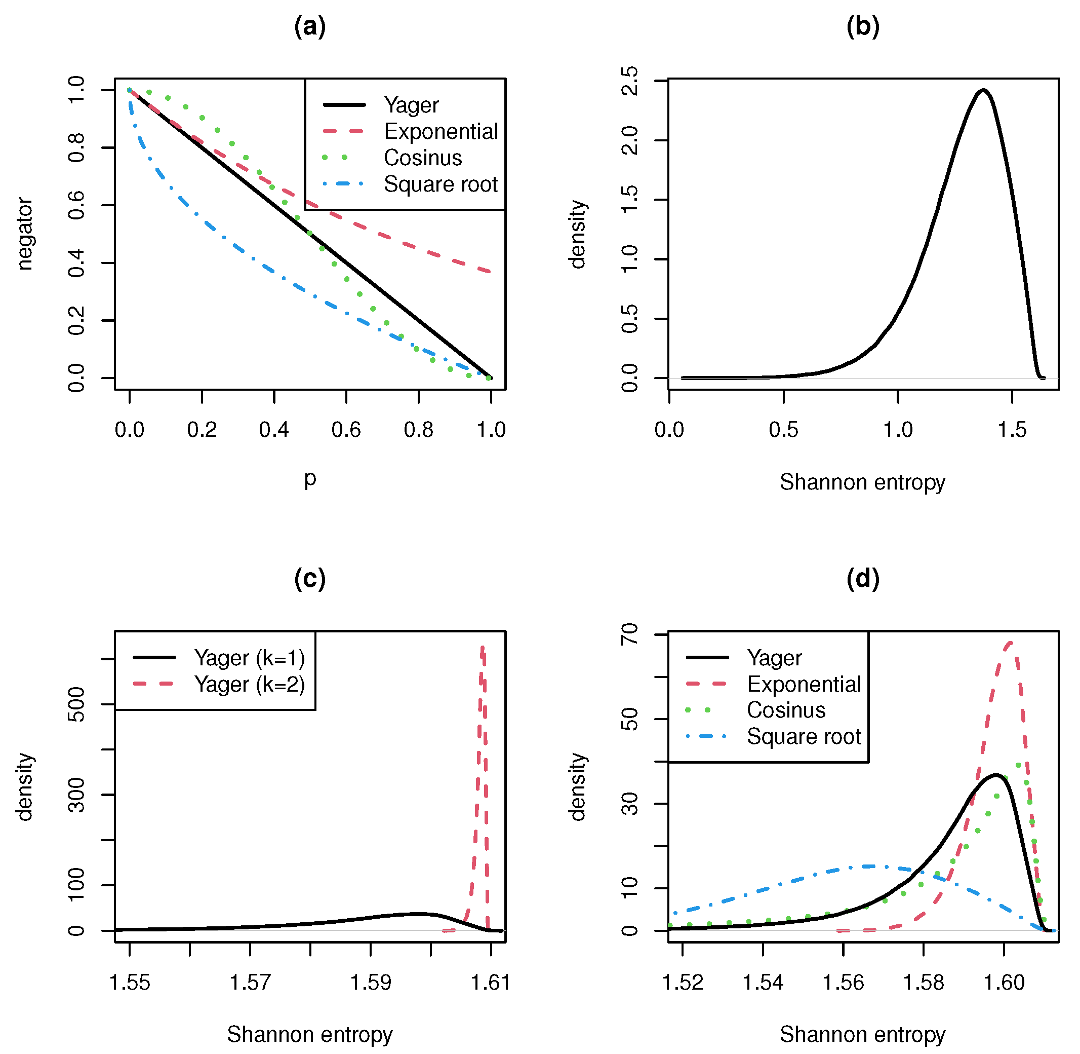
• Yager negator [1] $N_1$ with

  $$f_1\left(p\right)=1-p,0\le p\le 1,$$
• exponential negator [7] $N_2$ with

  $$f_2\left(p\right)=e^{-p},0\le p\le 1,$$
• cosinus negator $N_3$ with

  $$f_3\left(p\right)=0.5(cos\left(\pi p\right)),0\le p\le 1,$$
• and square root negator $N_4$ (special case of the Tsallis negator discussed by Zhang et al. [6]):

  $$f_4\left(p\right)=1-\sqrt{p},0\le p\le 1.$$

  $f_2$, $f_3$ and $f_4$ are generating functions for dependent negations. For dependent negations, it is not easy to prove properties of their entropies. Wu et al. [7] discussed the exponential negation. They considered the Shannon entropy for this negator. In their numerical examples, they compared Yager und exponential negators for different concrete probability vectors and a different number of categories n. Their general result is that exponential negator converges faster to the uniform distribution than Yager negator.

We choose another approach to get an idea how Gini and Shannon entropies behave for dependent negators and how fast the convergence is. We obtain 1,000,000 different probability vectors $p_1,\dots ,p_n$ by drawing random samples from a Dirichlet distribution. For each probability vector, the entropy (Gini or Shannon) is calculated. From the resulting 1,000,000 entropy values we estimate the entropy density. The same procedure is applied for the probability vectors transformed by the negators $N_i$, $i=1,2,3,4$. We use the random generator rdirichlet from the R-package ”MCMCpack” of [29] and density estimation by the standard R routine ”density”. Walley [30] discussed the Dirichlet distribution as a model for probabilities. The Dirichlet distribution has a vector of hyperparameters $({\alpha }_1,\dots ,{\alpha }_n)$ that has to be chosen before starting the simulation. Following [30], the decision falls on a noninformative prior setting with $\alpha =i=1$, $i=1,2,\dots ,n$. Note that other choices affect the graphical representation, but not the general results.

Figure 1 and Figure 2 show the results for the Gini resp. the Shannon entropy. The number of categories is in both cases $n=5$. For a higher number of categories, the results are even more pronounced. The top left panel presents the generating functions of the four negators. The top right panel shows the density estimation for the entropy of the original (non-transformed) probability vector. The bottom left panel compares the estimated entropy densities for the Yager negation applied once ($k=1$) and twice ($k=2$). The bottom right panel presents a comparison of the estimated entropy densities when the four negators are applied exactly once.

We can see that there is not much difference between the results for the Gini and the Shannon entropy. For $n=5$, the Gini entropy has the maximum value $0.8$ and the Shannon entropy the maximum value $ln5=1.609$. This explains the range of the abscissae.

The main results are:

• A single application of the negation already results in a very concentrated and strongly peaked entropy distribution. This confirms the fact stated in Remark 1 that the range of negations is very narrow.
• The double or multiple use of a negation leads to a distribution that resembles a singular distribution concentrated at the entropy’s maximum value. Therefore, the convergence rate to the uniform distribution is very high.
• The convergence rate is even higher when we consider negations with generating function f with $f\left(p\right)\ge f_1\left(p\right)$ for $0\le p\le 1$. The reverse is also true. Negations with generating function $f\left(p\right)\le f_1\left(p\right)$, $0\le p\le 1$ give lower convergence rates.
• In the interval $[0,1/2]$, the generating function of the cosinus negation is greater and in $[1/2,1]$ smaller than the generating function of the Yager negation. Nevertheless, the cosinus negation produces entropy distributions looking similar to the entropy distribution of the Yager negation. The entropy formula seems to eliminate the difference between the cosinus and the Yager negator.

8. Conclusions

First, we can prove that independent negations must be affine-linear. Due to Batyrshin [2] this was an open problem. The property of monotonicity means that the entropy cannot decrease by applying negation to a probability vector. This is equivalent to the fact that negations imply an information loss. We show that the property of monotonicity is satisfied for $\varphi$-entropies and Yager negation. It is sufficient to consider Yager negation because we can prove that the monotonicity of entropies of Yager negation can be transferred to all affine-linear (=independent) negations. We try to prove the monotonicity of $\varphi$-entropies by means of strict concavitiy of the entropy generating function. This procedure is only partially successful. The monotonicity holds for odd and even sequences for the number of negation repetitions k separately. Alternatively, following some examples from the literature, we try to prove monotonicity by a Lagrangian approach based on the difference of the $\varphi$-entropies for Yager negation and the original probability vector. For general $\varphi$-entropies, this approach is also only partially successful. We can prove monotonicity in the neighbourhood of the uniform distribution as the point where the difference of the $\varphi$-entropies has a local minimum. To show monotonicity for all probability vectors, we have to consider concrete $\varphi$-entropies like the Gini, the Shannon or the Havrda–Charvát (Tsallis) entropy. For the Gini entropy, it is not necessary to use the Lagrangian approach. The Gini entropy of an affine-linear negation can be represented as a convex combination of maximal Gini entropy and Gini entropy of the original probability vector. This updating formula can be applied to arbitrary k-times the negation is repeated. This leads to a sequence of non-decreasing values for Gini entropy converging towards the maximum value generated by the uniform distribution. Such an argument does not seem to apply for Shannon entropy. For this reason, we again take up the Lagrangian approach and show that the uniform distribution is the unique point at which the Lagrange function of Shannon entropy difference has a global minimum. The same can be shown for the difference of Havrda–Charvát (Tsallis) entropies. This means that the property of monotonicity is valid for Gini, Shannon and Havrda–Charvát (Tsallis) entropy. $(h,\varphi )$-entropies generalize $\varphi$-entropies. If h is a strictly increasing function and the condition of monotonicity holds for a $\varphi$-entropy, we show that the property of monotonicity is also satisfied for $(h,\varphi )$-entropy. With this argument, the property of monotonicity can easily be checked for Rényi and Sharma–Mittal entropy. For dependent negations, it is not easy to get analytical results. Therefore, we simulate the entropy distribution and show how different repeated negations affect Gini and Shannon entropy. The simulation approach has the advantage that the whole simplex of discrete probability vectors can be considered at once and not just arbitrarily selected probability vectors. When Yager negation is used as a point of reference, we see that negations with generating functions larger (smaller) than the generating function of Yager negation produce larger (smaller) information loss and a (lower) higher speed of convergence to the uniform distribution.

References

- Yager, R. On the maximum entropy negation of a probability distribution. IEEE Trans. Fuzzy Syst. 2014, 23, 1899–1902. [Google Scholar] [CrossRef]
- Batyrshin, I.; Villa-Vargas, L.A.; Ramirez-Salinas, M.A.; Salinas-Rosales, M.; Kubysheva, N. Generating negations of probability distributions. Soft Comput. 2021, 25, 7929–7935. [Google Scholar] [CrossRef]
- Batyrshin, I. Contracting and involutive negations of probability distributions. Mathematics 2021, 9, 2389. [Google Scholar] [CrossRef]
- Gao, X.; Deng, Y. The generalization negation of probability distribution and its application in target recognition based on sensor fusion. Int. J. Distrib. Sens. Netw. 2019, 15, 1–8. [Google Scholar] [CrossRef]
- Gao, X.; Deng, Y. The negation of basic probability assignment. IEEE Access 2019, 7, 107006–107014. [Google Scholar] [CrossRef]
- Zhang, J.; Liu, R.; Zhang, J.; Kang, B. Extension of Yager’s negation of a probability distribution based on Tsallis entropy. Int. J. Intell. Syst. 2020, 35, 72–84. [Google Scholar] [CrossRef]
- Wu, Q.; Deng, Y.; Xiong, N. Exponential negation of a probability distribution. Soft Comput. 2022, 26, 2147–2156. [Google Scholar] [CrossRef]
- Srivastava, A.; Maheshwari, S. Some new properties of negation of a probability distribution. Int. J. Intell. Syst. 2018, 33, 1133–1145. [Google Scholar] [CrossRef]
- Aczél, J. Vorlesungen über Funktionalgleichungen und ihre Anwendungen; Birkhauser: Basel, Switzerland, 1961. [Google Scholar]
- Ilić, V.; Korbel, J.; Gupta, S.; Scarfone, A. An overview of generalized entropic forms. Europhys. Lett. 2021, 133, 50005. [Google Scholar] [CrossRef]
- Burbea, J.; Rao, C. On the convexity of some divergence measures based on entropy functions. IEEE Trans. Inf. Theory 1982, 28, 489–495. [Google Scholar] [CrossRef]
- Salicrú, M.; Menéndez, M.; Morales, D.; Pardo, L. Asymptotic distribution of (h,Φ)-entropies. Commun. Stat. Theory Methods 1993, 22, 2015–2031. [Google Scholar] [CrossRef]
- Gini, C. Variabilità e Mutabilità: Contributo alla Distribuzioni e delle Relazioni Statistiche; Tipografia di Paolo Cuppin: Bologna, Italy, 1912. [Google Scholar]
- Onicescu, O. Théorie de l’information énergie informationelle. Comptes Rendus l’Academie Sci. Ser. AB 1966, 263, 841–842. [Google Scholar]
- Vajda, I. Bounds on the minimal error probability and checking a finite or countable number of hypotheses. Inf. Transm. Probl. 1968, 4, 9–17. [Google Scholar]
- Rao, C. Diversity and dissimilarity coefficients: A unified approach. Theor. Popul. Biol. 1982, 21, 24–43. [Google Scholar] [CrossRef]
- Shannon, C. A mathematical theory of communication. Bell Syst. Tech. J. 1948, 27, 379–423. [Google Scholar] [CrossRef]
- Havrda, J.; Charvát, F. Quantification method of classification processes. Concept of structural α-entropy. Kybernetika 1967, 3, 30–35. [Google Scholar]
- Daróczy, Z. Generalized information functions. Inf. Control. 1970, 16, 36–51. [Google Scholar] [CrossRef]
- Tsallis, C. Possible generalization of Boltzmann-Gibbs statistics. J. Stat. Phys. 1988, 52, 479–487. [Google Scholar] [CrossRef]
- Leik, R. A measure of ordinal consensus. Pac. Sociol. Rev. 1966, 9, 85–90. [Google Scholar] [CrossRef]
- Klein, I.; Mangold, B.; Doll, M. Cumulative paired ϕ-entropy. Entropy 2016, 18, 248. [Google Scholar] [CrossRef]
- Shafee, F. Lambert function and a new non-extensive form of entropy. IMA J. Appl. Math. 2007, 72, 785–800. [Google Scholar] [CrossRef]
- Mosler, K.; Dyckerhoff, R.; Scheicher, C. Mathematische Methoden für Ökonomen; Springer: Berlin, Germany, 2009. [Google Scholar]
- Rényi, A. On measures of entropy and information. In Proceedings 4th Berkeley Symposium on Mathematical Statistics and Probability; University of California Press: Berkeley, CA, USA, 1961; pp. 547–561. [Google Scholar]
- Sharma, B.; Mittal, D. New nonadditive measures of entropy for discrete probability distributions. J. Math. Sci. 1975, 10, 28–40. [Google Scholar]
- Uffink, J. Can the maximum entropy principle be explained as a consistency requirement? Stud. Hist. Philos. Sci. Part B Stud. Hist. Philos. Mod. Phys. 1995, 26, 223–261. [Google Scholar] [CrossRef]
- Jizba, P.; Korbel, J. When Shannon and Khinchin meet Shore and Johnson: Equivalence of information theory and statistical inference axiomatics. Phys. Rev. E 2020, 101, 042126. [Google Scholar] [CrossRef] [PubMed]
- Martin, A.; Quinn, K.; Park, J. MCMCpack: Markov Chain Monte Carlo in R. J. Stat. Softw. 2011, 42, 22. [Google Scholar] [CrossRef]
- Walley, P. Inferences From multinomal data: Learning sbout a bag of marbles (with discussion). J. R. Stat. Soc. Ser. B 1996, 58, 3–57. [Google Scholar]