Applications of the Delay Stochastic Simulation Algorithm (DSSA) in Mathematical Epidemiology

Abstract

The calculation of the probability of a minor outbreak is crucial in analyzing a stochastic epidemic model. For stochastic epidemic models with fixed delays, the linear chain trick is applied to transform the delayed models into a family of ODE models with increasing shape parameters. We then prove that the well-established results on the probability of a minor outbreak for continuous-time Markov chain (CTMC) epidemic models also hold for the stochastic epidemic models with fixed delays. All theoretical results are verified by numerical simulations implemented by the delay stochastic simulation algorithm (DSSA) in Python. It is shown that DSSA is able to generate exact realizations for underlying delayed models in the context of mathematical epidemiology, and therefore, provides insights into the effect of delays during the outbreak phases of epidemics.

1. Background and Motivation

Mathematical modeling of infectious disease transmissions and other population dynamics with delays is primarily based on the systems of delay differential Equations (DDEs). DDEs are also applied to study other biological and biochemical systems, e.g., viral infection ([1,2,3]), signal transduction ([4,5]) and gene expression in cellular systems ([6]). In mathematical epidemiology, time delays are considered to model mechanisms in the disease dynamics ([7]). Such mechanics of disease dynamics include latent period, infectious period, temporary immune period and so on. Epidemic models with such delays are formulated as systems of delay differential equations if the delays are considered fixed, or delay integral equations and delay integro-differential equations if delays are considered generally distributed. We refer to [7,8,9,10] for the relatively complete introductions of DDE models in epidemiology and population dynamics. In the research area of within-host modeling, delays are always referred as the eclipse phases. Inclusion of the eclipse phases is important in the study of the early infection stage of target cells, since the infected host cells may die or be cleared by the immune system prior to active viral production ([1,11]).

Stochastic modeling provides more accurate description of the behavior of biological systems when the quantity of the species size is small. Environmental variability and demographic variability are two major factors in stochastic modeling for the infectious diseases. Environmental variability is especially important in modeling zoonotic diseases, vector-borne diseases and waterborne diseases ([12,13]), and demographic variability associated with individual dynamics such as transmission, births, deaths and recovery is critical in analyzing the possible outcomes of the epidemics ([12,14]). In this paper, we mainly consider the effect of demographic variability on the early stage of an epidemic outbreak. For dynamical systems on the individual level, the same techniques of stochastic modeling can be applied once the assumption of mass action law holds ([15,16,17]). One of the most important topics in stochastic epidemic modeling is the calculation of the probability of a minor (major) epidemic outbreak. The terminology minor or major originates from [18] in the context of describing epidemic outbreaks ([12,19]). The definition of a minor outbreak in mathematical epidemiology is equivalent to the extinction in ecology, which is used to describe the evolutionary dynamics of generations for species under study. For stochastic epidemic models without delays, the probability of a minor outbreak can be estimated by the approximated multi-type branching process (BP) theory and the backward Kolmogorov differential equations, because the stochastic models can be studied as the multi-type continuous-time Markov chain (CTMC) processes ([12,19]). Numerically, the stochastic simulation algorithm (SSA), which was initially proposed by D.T.Gillespie in [15], describes the evolution of underlying stochastic Markov process. There are different versions of SSA, such as the original Gillespie’s first reaction algorithm ([15,16,17]), the next reaction algorithm ([20]) and the modified next reaction algorithm ([21]). SSA provides exact realizations for the underlying chemical master Equation (CME) of the corresponding stochastic process.

DDEs with fixed discrete delays can be treated as the limit of DDEs with distributed infinite delays of Gamma type when the shape parameter approaches infinity ([10]). It is well known that the Gamma distribution reduces to the Erlang distribution when the shape parameters are integers and becomes to the Dirac distribution when the shape parameter goes to infinity. Thus, it is natural to consider the DDEs with fixed delays as the limit model of a family of ODE models with increasing shape parameters $n=1,2,\cdots$. The delayed period is replaced by a sequential of identical sub-stages. For stochastic modeling, the delayed stochastic process can be analyzed through a family of stochastic Markov chain processes. This transformation technique is referred as the linear chain trick (LCT). LCT has been applied to study various of delayed epidemic models ([22,23,24]) and delayed within-host models ([1,2,3,25,26]). In [1], the authors formulated the delayed stochastic within-host model and its approximated stochastic Markov chain models by LCT, and analytically calculated the probability of a minor infection which initiated by a single infectious cell or latent cell or free virus. Unfortunately, the analytical results cannot be numerically verified due to the lack of the proper simulation methods. This is the motivation of the paper, which is to provide a general framework to calculate the analytical results and introduce the delay stochastic simulation algorithm (DSSA) to perform numerical simulations for the delayed stochastic epidemic models.

DSSA was developed in order to provide the exact realizations for underlying delayed biological models ([27]); however, so far, it has not brought too much attention in the community of mathematical epidemiology and population dynamics. Several versions of DSSA have been proposed since 2005. The first DSSA algorithm was proposed in [28]; however, it was proved that this algorithm has flaws ([29]). The rejection algorithm was later proposed in [30]. Another direct algorithm was proposed in [27]. It has been compared that both the rejection algorithm and direct algorithm are exact, but the rejection method needs to generate $50\%$ more random variables ([27]). A concise description of the direct algorithm is as follows and will be implemented to generate sample paths of underlying stochastic processes with delays. The state vector is denoted as X, and we suppose that there are $N_d$ ongoing reactions at time $t=T_0$, and the reactions will finish at time $t+T_1\le t+T_2\le \cdots \le t+T_{N_d}$. The interval $[T_i,T_{i+1})$ in which the next reaction will occur can be calculated by finding i that satisfies:

$$F_{\tau }\left(T_i\right)\le r\le F_{\tau }\left(T_{i+1}\right),$$

with:

$$F_{\tau }\left(\tau \right)=1-exp(-\sum _{j=0}^{i-1}{a}_0(t+T_j)(T_{j+1}-T_j)-a_0(t+T_i)(\tau -T_i)),\tau \in [T_i,T_{i+1}),$$

for $r\in U(0,1)$, $a_0\left(t\right)$ is the sum of all propensity functions at time t and $i=0,\cdots ,N_d$. The way to generate which type of reaction will be occurring is similar with the SSA.

The goal of this paper is to provide the general framework to calculate the probability of a minor outbreak for stochastic epidemic models with fixed delays, with the application of the linear chain trick and to introduce the delay stochastic simulation algorithm (DSSA) to perform numerical simulations in the area of modeling for infectious diseases. This paper is organized as follows: in Section 2, we formulate and analyze the general delayed stochastic epidemic model and a family of approximated continuous-time Markov chain (CTMC) models. In Section 3, we generate the convergence results regarding the delayed epidemic model and establish the results on the probability of a minor outbreak for the delayed model. In Section 4, several numerical simulations are performed in order to verify the analytical results we obtained in the previous sections. In Section 5, the conclusion is drawn and some possible future work is suggested.

2. Formulation and Analysis of the Delayed Epidemic Stochastic Model

We formulate and describe the delayed stochastic epidemic model (1), in which the delay $\tau$ accounts for the period for infected individuals to stay in the exposed stage. As the time scale of an epidemic outbreak is short enough to ignore demographic effects, factors such as population immigration will not be considered in our investigation. This model is an extension of the widely known general stochastic epidemic model, which was introduced by Barlett in 1949 ([31]):

$$\left\{\begin{array}{c}{\displaystyle \mathbf{Delayed}\mathbf{Event}:P(S_{t+\Delta t}-S_t=-1)=\frac{\beta }{N}SI+o(\Delta t),}\hfill \\ \mathbf{Non}-\mathbf{delayed}\mathbf{Event}:P((I_{t+\Delta t},R_{t+\Delta t})-(I_t,R_t)=(-1,1))={\gamma }_{I}I+o(\Delta t).\hfill \end{array}\right.$$

(1)

The random variable $(S_t,I_t,R_t)$ is the state vector to represent the sizes of susceptible class, infectious class and removed/recovered class at time t, respectively. N is a constant and is assumed as the size of the total population and the contact rate is assumed to $\beta >0$. Removal rate for the infectious class is set to ${\gamma }_I>0$. The first event of the model is delay related and if it occurs, we have $S_t-1$ immediately and after an exact period of delay $\tau$ there are two possible outcomes. With the probability of $e^{-{\gamma }_E\tau }$, $I(t+\tau )-I\left(t\right)=1$; and with the probability of $1-e^{-{\gamma }_E\tau }$, $R(t+\tau )-R\left(t\right)=1$. ${\gamma }_E$ is the removal rate for individuals in the exposed stage. The two probabilities are both determined by ${\gamma }_E$. A compartmental diagram of the model (1) is presented in Figure 1.

If the removal rate ${\gamma }_E$ is considered nonzero for the delayed event, a third random variable needs to be generated computationally to account for two different outcomes, which is compared to Gillespie’s algorithm ([16,17]). We will discuss this method in the section of numerical simulations. With reasonable minor modifications, we are able to avoid generating the third random variable. Although it is not theoretically necessary, this modification is able to slightly speed up the numerical computations. It is also noted that the exposed stage in this stochastic epidemic model is intermediate and is included implicitly.

The basic reproduction number for the delayed stochastic epidemic model (1) is:

$${\mathcal{R}}_0^d=\frac{\beta }{{\gamma }_I}{e}^{-{\gamma }_E\tau },$$

(2)

the superscript d indicates for the case of fixed delays. It is well known that for stochastic epidemic models without delays or the CTMC models, ${\mathcal{R}}_0$ plays a central role in determining the probability of a minor outbreak. When the epidemic is initiated with i infectious cases, if ${\mathcal{R}}_0>1$ we have ${\mathbb{P}}_{minor}={\left(\frac{1}{{\mathcal{R}}_0}\right)}^i$ and while if ${\mathcal{R}}_0<1$, ${\mathbb{P}}_{minor}=1$ ([12]). We will establish the analogous results for stochastic epidemic models with delays.

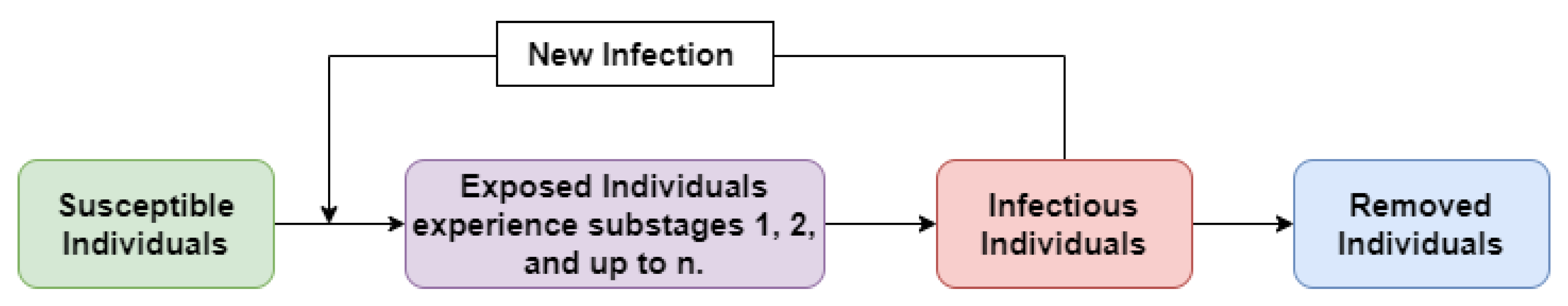
We next formulate the following family of approximated CTMC models (3) with explicit exposed sub-stages. The number of exposed sub-stages n is ranged from 1 to ∞. The random variable $(S_t,E_{1,t},\cdots ,E_{n,t},I_t,R_t)$ is the vector to represent the sizes of susceptible class, exposed sub-stages indexed from 1 to n, infectious class and recovered class at time t. For sake of simplicity, only related compartments are involved in probability (infinitesimal transition rate) definitions.

$$\left\{\begin{array}{c}P((S_{t+\Delta t},E_{1,t+\Delta t})-(S_t,E_{1,t})=(-1,1))=\frac{\beta }{N}{S}_t{I}_t+o(\Delta t),\hfill \\ P((E_{1,t+\Delta t},E_{2,t+\Delta t})-(E_{1,t},E_{2,t})=(-1,1))=n\delta E_{1,t}+o(\Delta t),\hfill \\ ⋮\hfill \\ P((E_{n-1,t+\Delta t},E_{n,t+\Delta t})-(E_{n-1,t},E_{n,t})=(-1,1))=n\delta E_{n-1,t}+o(\Delta t),\hfill \\ P((E_{n,t+\Delta t},I_{t+\Delta t})-(E_{n,t},I_t)=(-1,1))=n\delta E_{n,t}+o(\Delta t),\hfill \\ P((E_{1,t+\Delta t},R_{t+\Delta t})-(E_{1,t},R_t)=(-1,1))={\gamma }_E{E}_{1,t}+o(\Delta t),\hfill \\ ⋮\hfill \\ P((E_{n,t+\Delta t},R_{t+\Delta t})-(E_{n,t},R_t)=(-1,1))={\gamma }_E{E}_{n,t}+o(\Delta t),\hfill \\ P((I_{t+\Delta t},R_{t+\Delta t})-(I_t,R_t)=(-1,1))={\gamma }_I{I}_t+o(\Delta t).\hfill \end{array}\right.$$

(3)

The compartmental diagram of the model (3) is presented in Figure 2.

All complementary probabilities are omitted in model (3). There are $2n+2$ events. The first event represents the appearance of a new infected case. The following events represent the transmission from one exposed sub-stage to the next exposed sub-stage, and the removals from each exposed sub-stage, respectively. The transition rates from one exposed sub-stage to the next one is $n\delta$ and ${\displaystyle \delta =\frac{1}{\tau }}$. The last event accounts for the removal from the infectious class. In the context of computational biology, the defined probabilities in model (3) are also called the propensity functions of reactions. The underlying assumption of the CTMC model (3) is that the inter-event time is exponentially distributed with parameter W is:

$$W=\frac{\beta }{N}{S}_t{I}_t+(n\delta +{\gamma }_E)\sum _{i=1}^n{E}_{i,t}+{\gamma }_I{I}_t.$$

(4)

With $n=1$, the stochastic epidemic model (3) can be reduced to the simple SEIR stochastic compartmental model. In the counterpart of deterministic modeling, such epidemic models with delays are formulated as systems of delay differential equations and are often studied by families of systems of ordinary differential equations. It is followed by linear chain trick and is based on the fact that the Dirac distribution is the limit of the Erlang distributions:

$${\displaystyle f(x;,n,n{\gamma }_E)=\frac{{\left(n{\gamma }_E\right)}^n}{(n-1)!}{x}^{(n-1)}{e}^{-n{\gamma }_{E}x},x>0,n\in \mathbb{N},}$$

(5)

when the shape parameter goes to infinity ([1,10]). n is the shape parameter and $n{\gamma }_E$ is the scale parameter. When $n=1$, the Erlang distribution reduces to an exponential distribution. The basic reproduction numbers for the stochastic models (3) can be expressed as:

$${\mathcal{R}}_0^n=\frac{\beta }{{\gamma }_I}{\left(\frac{n\delta }{n\delta +{\gamma }_E}\right)}^n,$$

(6)

the superscript n represents the number of exposed sub-stages considered. It is also straightforward to verify that ${\displaystyle \underset{n\to \infty }{lim}{\mathcal{R}}_0^n={\mathcal{R}}_0^d}$ in (2).

Remark 1.

${\mathcal{R}}_0^n$ is monotonically decreasing as n increases, the series of ${\mathcal{R}}_0^n$ is lower bounded by its limit ${\mathcal{R}}_0^d$. Even with the same mean exposed stage, it is possible that ${\mathcal{R}}_0^n$ decreases from above 1 to below 1 as n increases. Thus, the assumptions on the structure of exposed stage may cause a dramatic change of dynamical behavior of the early stage. The following Figure 3 shows one example of the change of ${\mathcal{R}}_0^n$ as n increases. When the distribution shape parameters $n=1$ and $n=2$, the corresponding basic reproduction number ${\mathcal{R}}_0^n>1$, while if $n\ge 3$, the basic reproduction number ${\mathcal{R}}_0^n<1$. It is noticed that the combination of parameter values is carxefully chosen in order to guarantee that the value of ${\mathcal{R}}_0^1$ is slightly larger than 1. This might be critical in epidemic model selection regards to the distribution of periods of exposed stages, but only for some very restrictive cases that ${\mathcal{R}}_0^n$ is rather close to 1.

3. The Approach to Calculate the Minor Outbreak Probability

The Branching Process (BP) estimates come from a multi-type birth and death linear approximation of the Markov chain model near the disease-free equilibrium ([19,32]):

$$(S,E_1,E_2,\cdots ,E_n,I,R)=(N,0,0,\cdots ,0,0).$$

The BP approximation is reasonable during the early stage of an epidemic ([1,19,32]). A probability generating function (pgf) corresponding to $(n+1)$ variables $E_1,\cdots ,E_n,I$, representing the number of offspring of type $E_k$ ($k=1,\cdots ,n$) and I, generating from 1 exposed individual in different exposed sub-stage or 1 infectious individual. The domain of the pgfs is $u\in {[0,1]}^{n+1}$, where $u=(u_1,\cdots ,u_{n+1})$. The pgf $f_1\left(u\right)$ is the pgf for individuals in the first exposed sub-stage $E_1$ given $E_1\left(0\right)=1,E_2\left(0\right)=\cdots =E_n\left(0\right)=I\left(0\right)=0$. The same interpretations for $f_2\left(u\right),f_3\left(u\right),\cdots ,f_{n+1}\left(u\right)$ can be made. The pgf for $n+1$ states are defined as below:

$$\begin{array}{cc}\hfill f_i(u_1,u_2,\cdots ,u_{n+1})& {\displaystyle =\frac{n\delta u_{i+1}+{\gamma }_E}{n\delta +{\gamma }_E},i=1,2,\cdots ,n}\hfill \\ \hfill f_{n+1}(u_1,u_2,\cdots ,u_{n+1})& {\displaystyle =\frac{\beta u_1{u}_{n+1}+{\gamma }_I}{\beta +{\gamma }_I}.}\hfill \end{array}$$

(7)

It is well known that there is at least one fixed point of the pgfs in the domain $u\in {[0,1]}^{n+1}$, namely, $(1,1,...,1)$. However, there exists at least one more fixed point when ${\mathcal{R}}_0^n>1$, ${\mathcal{R}}_0^n$ is defined in Equation (6). It follows from the theory of multi-type branching process that the minimal fixed point of the pgfs $(q_1,...,q_{n+1})$ is the asymptotic estimate for the probability of a minor outbreak given either one latent individual or one infectious individual ([32,33]). Thus, for the random variable $X\left(t\right)$ corresponding to the $n+1$ disease-related variables, and $X\left(0\right)=(0,0,\cdots ,0,1,0,\cdots ,0)$ with 1 the i-th element represents the initial condition of one exposed individual in exposed sub-stage i or one infectious individual, the conditional probability of a minor outbreak of an epidemic is defined as:

$$\underset{t\to \infty }{lim}P(X\left(t\right)=0|X\left(0\right))=q_i.$$

(8)

Theorem 1.

In the multi-type branching process approximation, assume there is one exposed individual in one specific exposed sub-stage or one infectious individual, representing stage $i\in \{1,2,\cdots ,n+1\}$. If the basic reproduction number ${\mathcal{R}}_0^n<1$ then the probability of a minor outbreak is $\mathbb{P}=1$ and if ${\mathcal{R}}_0^n>1$, the probability of a minor outbreak is $\mathbb{P}=q_i$. $q_i$ is defined as the fixed point of Equation (7).

The complete proof can be found in [12] by assuming the independence of multi-type branching process and by applying the backward Kolmogorov differential equations for the branching process approximation. In addition, it has been proved that if ${\mathcal{R}}_0^n<1$, the fixed point $(1,\cdots ,1)$ is stable and if ${\mathcal{R}}_0^n>1$, the fixed point $(q_1,q_2,\cdots ,q_{n+1})$ in the domain of ${(0,1)}^{n+1}$ exists and it is stable.

Next, we have the following convergence result,

Lemma 1.

The stochastic process (1) is the limit of the stochastic processes (3) when $n\to \infty$.

Proof. 

It is easy to check that two events $P(S_{t+\Delta t}-S_t=-1)$ and $P((I_{t+\Delta t},R_{t+\Delta t})-(I_t,R_t)=(-1,1))$ in both (1) and (3) are irrelevant to the number of exposed sub-stages n, and the propensity functions for both events are not changed. We then calculate two probabilities of outcomes if the first event occurs. Two possible outcomes are the infected individual successfully surviving through the exposed stage then entering the infectious stage, and the infected individual leaving the exposed stage before becoming contagious. The probabilities for two outcomes are, respectively:

$${\mathbb{P}}_1={\left(\frac{n\delta }{n\delta +{\gamma }_E}\right)}^n,{\mathbb{P}}_2=1-{\left(\frac{n\delta }{n\delta +{\gamma }_E}\right)}^n,$$

(9)

It then implies that:

$$\underset{n\to \infty }{lim}{\mathbb{P}}_1=e^{-{\gamma }_E\tau },\underset{n\to \infty }{lim}{\mathbb{P}}_2=1-e^{-{\gamma }_E\tau }.$$

(10)

□

The above theorem allows us to analyze the behaviors of the delayed stochastic model (1) by studying the family of CTMC models (3). Thus, in order to calculate the probability of a minor outbreak for model (1), we apply the multi-type branching process (BP) theory to approximate the CTMC models (3) near the disease-free equilibrium ([1,12,19,32]) and then take the limit of $n\to \infty$.

Theorem 2.

For delayed stochastic epidemic model (1), the probability of a minor epidemic outbreak by initially introducing i infectious cases ($i\ge 1$) is:

$${\mathbb{P}}_{minor}={\left(\frac{1}{{\mathcal{R}}_0^d}\right)}^i,$$

(11)

with ${\displaystyle {\mathcal{R}}_0^d=\frac{\beta }{{\gamma }_I}{e}^{-{\gamma }_E\tau }}$ representing the basic reproduction number for model (1).

Proof. 

We first analyze the approximated CTMC models (3). The analytical solution $(q_1,q_2,\cdots ,q_{n+1})$ is the fixed point for Equation (7), which can be expressed explicitly as:

$$\left\{\begin{array}{c}{\displaystyle \frac{n\delta q_2+{\gamma }_E}{n\delta +{\gamma }_E}=q_1,}\hfill \\ ⋮\hfill \\ {\displaystyle \frac{n\delta q_{n+1}+{\gamma }_E}{n\delta +{\gamma }_E}=q_n,}\hfill \\ {\displaystyle \frac{\beta q_1{q}_{n+1}+{\gamma }_I}{\beta +{\gamma }_I}=q_{n+1}.}\hfill \end{array}\right.$$

(12)

With suitable re-arrangement of the above system, we have:

$$\left\{\begin{array}{c}n\delta q_2+{\gamma }_E=q_1(n\delta +{\gamma }_E),\hfill \\ n\delta q_3+{\gamma }_E=q_2(n\delta +{\gamma }_E),\hfill \\ ⋮\hfill \\ n\delta q_{n+1}+{\gamma }_E=q_n(n\delta +{\gamma }_E),\hfill \\ \beta q_1{q}_{n+1}+{\gamma }_I=q_{n+1}(\beta +{\gamma }_I).\hfill \end{array}\right.$$

(13)

Simple computation indicates that the solution of the above system can be expressed as the following recursive formula:

$$\left\{\begin{array}{c}{\displaystyle q_{n+1}=\frac{{\gamma }_I}{\beta }{\left(\frac{n\delta +{\gamma }_E}{n\delta }\right)}^n=\frac{1}{{\mathcal{R}}_0^n},}\hfill \\ {\displaystyle q_1=\frac{\beta +{\gamma }_I}{\beta }-{\left(\frac{n\delta +{\gamma }_E}{n\delta }\right)}^n,}\hfill \\ {\displaystyle q_i=\frac{n\delta +{\gamma }_E}{n\delta }{q}_{i-1}-\frac{{\gamma }_E}{n\delta },i=2,\cdots ,n.}\hfill \end{array}\right.$$

(14)

Next, we take the limit $n\to \infty$ for $q_{n+1}$ in (14) and denote $q_I:=q_{n+1}$, the probability of a minor outbreak by initially introducing one infectious individual, for the delayed stochastic epidemic model (1) is ${\displaystyle \frac{1}{{\mathcal{R}}_0^d}}$. If the outbreak is initiated with i individuals and we assume that each infectious individual is independent from all other infectious individuals ([19,32]), it is naturally to have the probability of a minor outbreak equals to ${\left({\displaystyle \frac{1}{{\mathcal{R}}_0^d}}\right)}^i$, as desired. □

If we denote:

$${\displaystyle q_E:=\underset{n\to \infty }{lim}{q}_1=e^{-\tau {\gamma }_E}\frac{1}{{\mathcal{R}}_0^d}+(1-e^{-\tau {\gamma }_E})}$$

(15)

the probability of a minor outbreak by initially introducing one exposed individual. The term ${\displaystyle {\left(\frac{n\delta }{n\delta +{\gamma }_E}\right)}^n}$ in Equation (14) is the probability that the exposed individual successfully enters the infectious stage. If this exposed individual ends the latency and enters the removal class before turning into infectious, it is obvious that the major outbreak will not occur and we have a minor disease outbreak instead. It is also noticed that $q_i$ with $i=1,\cdots ,n-1$ can be expressed in the form of the conditional probability $q_{i+1}$:

$$q_i=p(i+1|i)q_{i+1}+(1-p(i+1|i)),$$

(16)

with ${\displaystyle p(i+1|i):=\frac{n\delta }{n\delta +{\gamma }_E}}$ representing the conditional probability of entering exposed sub-stage $i+1$ by assuming the individual has entered exposed sub-stage i. However, in practice, it is difficult to measure initially which sub-stage the exposed individual is in. We mainly focus on the case that the epidemic outbreak is initiated by a few infectious cases.

The result can be applied for more complicated types of stochastic epidemic models with fixed delays, such as the vector-borne stochastic models or the within-host stochastic models. Some analysis for the within-host stochastic viral infection model was performed in [1].

4. Applications of DSSA in Mathematical Epidemiology

The implementation of delay stochastic simulation algorithm (DSSA) is the main focus of this paper. First of all, we introduce two important definitions in DSSA, i.e., non-consuming reaction and consuming reaction ([21,27,29,34]),

Definition 1

(Non-consuming reaction). The reactants of an unfinished reaction can further participate in a new reaction.

Definition 2

(Consuming reaction). The reactants of an unfinished reaction cannot further participate in a new reaction.

It is noted that, in [21], two types of reactions are also named completion delayed reaction and initiation completion delayed reaction. In delayed stochastic modeling, it is crucial to distinguish the type of delayed reaction. For consuming reactions, there are updates of states at both initiation time and the completion time, while for nonconsuming reactions, the system only needs to be updated at the completion time. In applications of DSSA in epidemiology, it is arguably that nearly all delayed events considered are categorized as consuming events. Because once the individual is infected, this individual immediately enters the exposed stage and can not be reinfected. For epidemics such as the current COVID-19 pandemic, the infected individuals are initially asymptomatic and are able to further infect more susceptibles. For such cases, the event/reaction that susceptible individuals are infected by asymptomatic individuals is also consuming.

Similarly with the algorithm of SSA, the DSSA answers the following two questions:

(1)

When will the next event (reaction) occur?

(2)

Which event is the next event?

To be more specific, the DSSA simulates that no event occurs in the time interval $[t,t+\tau )$ and an event $R_{\mu }$ occurs in the infinitesimal time interval $[t+\tau ,t+\tau +d\tau )$. $\tau$ and $\mu$ are two independent random variables, and the probability density functions of $\tau$ and $\mu$ are given in [27]. Detailed derivations and pseudo-codes can also be found in [27,34].

Different from the numerical examples which are presented in [27] and in many other publications, we consider the removal rate in the fixed-delay exposed stage is nonzero. This slightly complicates the stochastic simulations, because if a delayed event occurs, there needs to be a third random variable to determine two possible outcomes after the fixed time of delay. The exposed individual either becomes infectious or leaves the latency period and enters the removal class. The ratio of probabilities of two outcomes, for the delayed epidemic model (1), is:

$${\displaystyle \mathrm{ratio}=\frac{e^{-{\gamma }_E\tau }}{1-e^{-{\gamma }_E\tau }}.}$$

To avoid generating one more random variable in implementations of DSSA, we modify the delayed stochastic epidemic model (1). The equivalent stochastic epidemic model can be written as:

$$\left\{\begin{array}{c}{\displaystyle \mathrm{Event}1:P(S_{t+\Delta t}-S_t=-1)=e^{-{\gamma }_E\tau }\frac{\beta }{N}SI+o(\Delta t),}\hfill \\ {\displaystyle \mathrm{Event}2:P(S_{t+\Delta t}-S_t=-1)=(1-e^{-{\gamma }_E\tau })\frac{\beta }{N}SI+o(\Delta t),}\hfill \\ \mathrm{Event}3:P((I_{t+\Delta t},R_{t+\Delta t})-(I_t,R_t)=(-1,1))={\gamma }_{I}I+o(\Delta t).\hfill \end{array}\right.$$

(17)

In this stochastic epidemic model, events 1 and 2 are delay related. If event 1 occurs at time t, one susceptible individual is immediately infected and becomes exposed. After a fixed duration of $\tau$ in latency, this individual becomes infectious. Thus, we have $I_{t+\tau }-I_t=1$. Similarly if event 2 occurs at time t, we have $R_{t+\tau }-R_t=1$. The exposed stage is an intermediate state, and all individuals in latency can not participate in any other events. The ratio of propensity functions of event 1 and event 2 is unchanged comparing with the original delayed stochastic model (1). It can be verified that model (17) and model (1) are equivalent, because the underlying sample spaces and their associated probabilities are identical for both stochastic processes.

We present the parameter values for the delayed stochastic epidemic model (1) in

Table 1. Parameter values for delayed stochastic epidemic model (1). The fixed delay in exposed stage is 2 days.

Parameter	Value
$\beta$	$0.5$ per day
$\delta$ ($\tau$)	$0.5$ per day (2 days)
${\gamma }_E$	$0.2$ per day
${\gamma }_I$	$0.2$ per day
N	$5\times {10}^3$

for numerical simulations. All numerical simulations (performed by the DSSA and the SSA) will be implemented in Python package StochPy ([35]).

The basic reproduction numbers for the delayed stochastic epidemic model and for the approximated CTMC epidemic models are:

$${\mathcal{R}}_0^d=1.676,{\mathcal{R}}_0^n=2.5\times {\left(\frac{0.5n}{0.5n+0.2}\right)}^n.$$

(18)

We perform three sets of numerical experiments to simulate the delayed stochastic processes described in model (1), and then numerically verify the result on the probability of a minor outbreak for the model, which was presented in Theorem 2. We also compare the result for the delayed stochastic epidemic model (17) (or equivalent model (1)) with the ones for the approximated CTMC models (3). It is noticed that the delayed epidemic model (1) (or model (17)) is simulated with the DSSA and the approximated stochastic models (3) are simulated with the SSA.

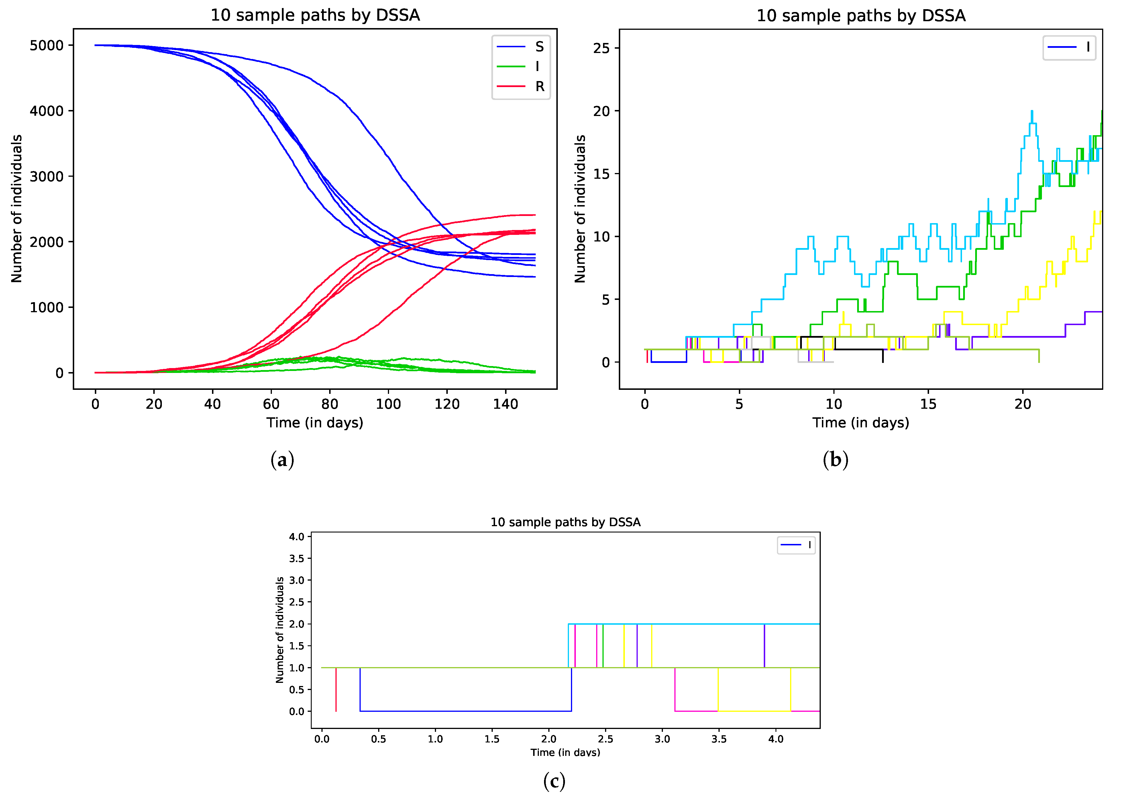
In the first set of simulations, we generate 10 realizations to illustrate the dynamics of the delayed stochastic model and investigate how the fixed delay affects the outbreak. The result of simulations is presented in Figure 4. Figure 4a presents 10 realizations; half of them represent major outbreaks, while the others represent minor outbreaks. Figure 4b is the zoomed-in view of the 10 realizations, it clearly shows that the numbers of infectious individuals hits 0 fast for realizations representing a minor outbreak. Figure 4c shows that all new infectious cases occur at the time which is later than day 2. This is due to the inclusion of the fixed delay for the exposed stage.

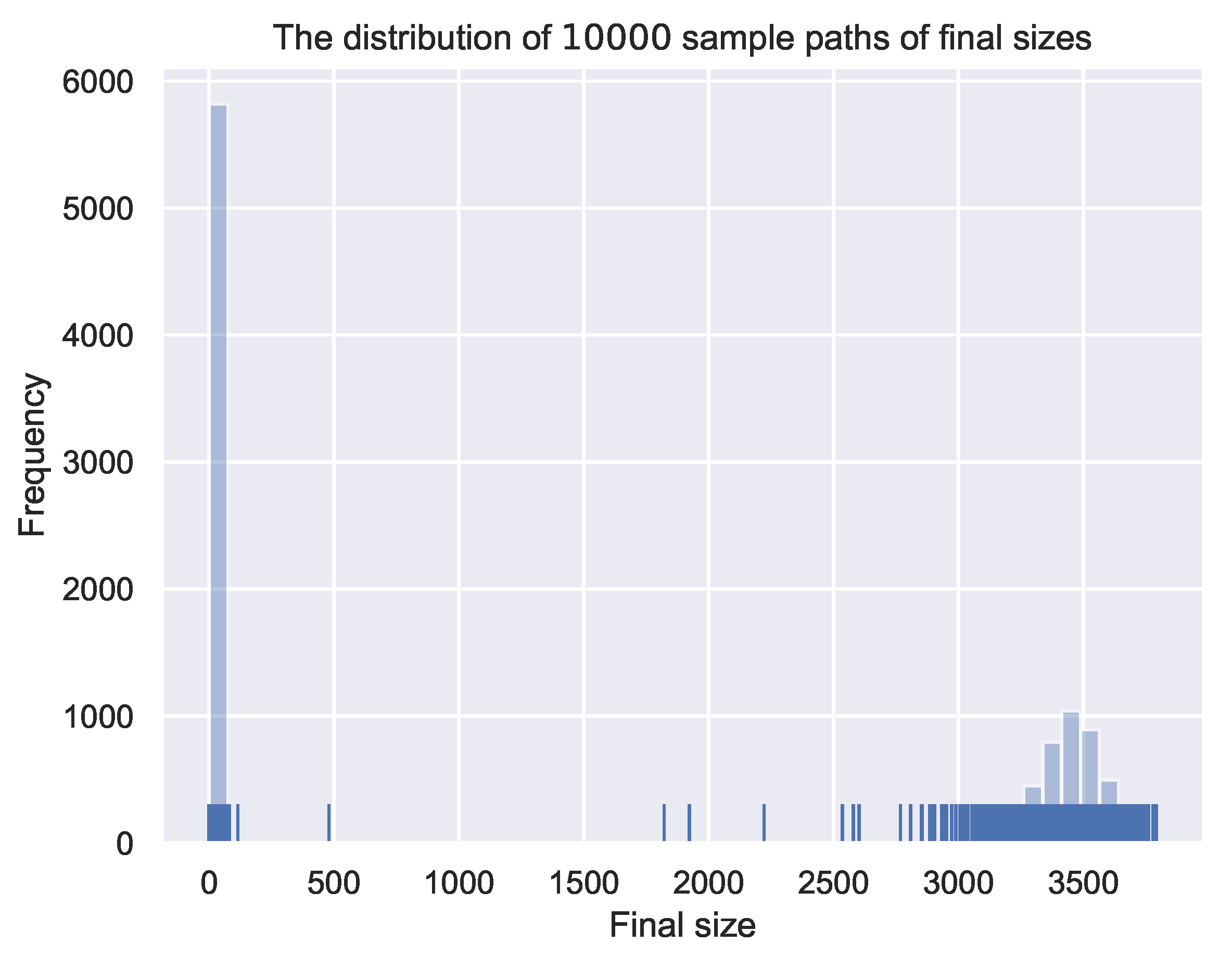
The second set of numerical simulations is to generate ${10}^4$ realizations by DSSA and estimate the probability of a minor outbreak by statistically summarizing the final sizes of all realizations, which is $S\left(\mathrm{initial} \mathrm{time}\right)-S\left(\mathrm{final} \mathrm{time}\right)$. We consider two initial conditions of one infectious individual and two infectious individuals. If the final epidemic size is less than the pre-defined threshold 50, we consider there to be a minor outbreak, while if the final epidemic size is larger, we consider there to be a major outbreak. Other pre-defined thresholds with relatively small values also work. This is because the distributions of final sizes for stochastic epidemic models are known as bimodal, and thus, there are very few falling in between.

The result of the simulations is presented in Figure 5. Figure 5a,b are the distributions of the final epidemic sizes of ${10}^4$ realizations for the delayed stochastic model (1) with initially one infectious individual and two infectious individuals, respectively. For Figure 5a, there are 5910 out of ${10}^4$ realizations, with the final sizes falling in interval $[0,50]$. If we reset the pre-defined threshold to 100, there are 5931 realizations with the final sizes falling in interval $[0,100]$. The distribution of the final sizes indicates that the probability of a minor outbreak is around $0.593$. By Theorem 2, we calculate that the probability of a minor outbreak by BP is ${\displaystyle {\mathbb{P}}_{minor}=\frac{1}{{\mathcal{R}}_0^d}=0.596}$. This shows a good agreement and proves that DSSA is able to generate exact realizations for underlying delayed stochastic epidemic models. For Figure 5b, if we set the pre-defined threshold value 100, there are 3521 realizations with the final sizes falling in interval $[0,100]$. This indicates that the estimated probability of a minor outbreak is around $0.352$, which has a good agreement with the probability calculated by BP: ${\mathbb{P}}_{minor}={\left({\displaystyle \frac{1}{{\mathcal{R}}_0^d}}\right)}^2=0.355$.

The third set of numerical simulations is to generate ${10}^4$ realizations for the approximated CTMC epidemic models (3) with with $n=1,2,5,10$. The initial condition is $I\left(0\right)=1$. Probabilities of a minor outbreak for stochastic epidemic models are indicated by the distributions of final epidemic sizes. We use the SSA to generate exact realizations for these stochastic models. The distributions of the final sizes for stochastic epidemic models are presented in Figure 6, Figure 7, Figure 8 and Figure 9. Therefore, the probabilities of a minor outbreak for the CTMC models (3) with $n=1,2,5,10$ can be obtained accordingly. We summarize the results in

Table 2. Comparison of probabilities of a minor outbreak for the stochastic epidemic models (3) with $n=1,2,5,10$, estimated by BP and by distributions of final sizes of ${10}^4$ realizations generated by SSA, respectively.

Number of Exposed Sub-Stages	BP Estimates	(D)SSA Estimates
$n=1$	$0.560$	$0.552$
$n=2$	$0.576$	$0.565$
$n=5$	$0.588$	$0.580$
$n=10$	$0.592$	$0.590$
$n=\infty$	$0.596$	$0.593$

. It can be observed that the results estimated from BP theory and the results generated by SSA show good agreement. With the increasing value of n, the probabilities of a minor outbreak increase and will converge to the probability for the delayed stochastic model (1). The result for the delayed stochastic model (1) is presented in the last row of Table 2.

5. Conclusions and Future Work

Continuous-time Markov Chain (CTMC) is the common modeling technique to estimate the probability of a minor outbreak for studying the early phases of infectious diseases in mathematical epidemiology. For delayed stochastic epidemic models, a family of CTMC models can be formulated and be used to approximate for the delayed model. By applying the methods of branching process theory (BP) and probability generating function (pgf) for the approximated CTMC models, and taking the limit as the number of exposed sub-stages $n\to \infty$ of the probabilities of a minor outbreak for the CTMC models, theoretical results on the probability of a minor outbreak for the delayed stochastic model can be established. Numerical simulations by stochastic simulation algorithm (SSA) and delay stochastic simulation algorithm (DSSA) are implemented in Python package StochPy. In implementations of DSSA, due to the existence of removal rate in the fixed length of exposed stage, we slightly modified the stochastic models by dividing the delayed event into two separate ones. This technique generates one more event, but successfully avoids the third random variable in the simulation process. The numerical results and the analytical results show good agreement. DSSA is a useful and powerful tool to generate exact realizations to study the underlying stochastic processes with delays in mathematical epidemiology.

There are many open problems in the study of delayed stochastic epidemic models and the simulations. Some deterministic epidemic models include transition phases following the distributed delays, and can be written in the form of systems of integro-differential equations with certain types of kernel functions. For such cases, the first technical difficulty is the formulation of the corresponding delayed stochastic epidemic models. Linear chain trick is no longer in use for such cases. The analysis on the probability of a minor outbreak for such delayed stochastic epidemic models is surely challenging as well.

References

Bai, F.; Huff, K.E.S.; Allen, L.J.S. The effect of delay in viral production in within-host models during early infection. J. Biol. Dyn.2018, 13, 47–73. [Google Scholar] [CrossRef] [PubMed]
Bai, F.; Allen, L.J. Probability of a major infection in a stochastic within-host model with multiple stages. Appl. Math. Lett.2019, 87, 1–6. [Google Scholar] [CrossRef]
Yan, A.W.C.; Cao, P.; McCaw, J.M. On the extinction probability in models of within-host infection: The role of latency and immunity. J. Math. Biol.2016, 73, 787–813. [Google Scholar] [CrossRef]
MIZUTANI, T. Signal Transduction in SARS-CoV-Infected Cells. Ann. New York Acad. Sci.2007, 1102, 86–95. [Google Scholar] [CrossRef]
Kang, C.C.; Chuang, Y.J.; Tung, K.C.; Chao, C.C.; Tang, C.Y.; Peng, S.C.; Wong, D.S.H. A genetic algorithm-based boolean delay model of intracellular signal transduction in inflammation. BMC Bioinform.2011, 12, S17. [Google Scholar] [CrossRef]
Li, P.; Li, Y.; Gao, R.; Xu, C.; Shang, Y. New exploration on bifurcation in fractional-order genetic regulatory networks incorporating both type delays. Eur. Phys. J. Plus2022, 137, 598. [Google Scholar] [CrossRef]
Arino, J.; van den Driessche, P. Time Delays in Epidemic Models. In Delay Differential Equations and Applications; Springer: Dordrecht, The Netherlands, 2006; pp. 539–578. [Google Scholar] [CrossRef]
Bacaër, N. A Short History of Mathematical Population Dynamics; Springer: London, UK, 2011. [Google Scholar] [CrossRef]
Brauer, F.; Castillo-Chavez, C. Mathematical Models in Population Biology and Epidemiology; Springer: New York, NY, USA, 2012. [Google Scholar] [CrossRef]
Smith, H. An Introduction to Delay Differential Equations with Applications to the Life Sciences; Springer: New York, NY, USA, 2011. [Google Scholar] [CrossRef]
Rong, L.; Gilchrist, M.A.; Feng, Z.; Perelson, A.S. Modeling within-host HIV-1 dynamics and the evolution of drug resistance: Trade-offs between viral enzyme function and drug susceptibility. J. Theor. Biol.2007, 247, 804–818. [Google Scholar] [CrossRef]
Allen, L. A primer on stochastic epidemic models: Formulation, numerical simulation, and analysis. Infect. Dis. Model.2017, 2, 128–142. [Google Scholar] [CrossRef]
Bittihn, P.; Golestanian, R. Stochastic effects on the dynamics of an epidemic due to population subdivision. Chaos Interdiscip. J. Nonlinear Sci.2020, 30, 101102. [Google Scholar] [CrossRef]
Black, A.J.; McKane, A.J. Stochasticity in staged models of epidemics: Quantifying the dynamics of whooping cough. J. R. Soc. Interface2010, 7, 1219–1227. [Google Scholar] [CrossRef]
Gillespie, D.T. A general method for numerically simulating the stochastic time evolution of coupled chemical reactions. J. Comput. Phys.1976, 22, 403–434. [Google Scholar] [CrossRef]
Gillespie, D.T. Exact stochastic simulation of coupled chemical reactions. J. Phys. Chem.1977, 81, 2340–2361. [Google Scholar] [CrossRef]
Gillespie, D.T. Gillespie Algorithm for Biochemical Reaction Simulation. In Encyclopedia of Computational Neuroscience; Springer: New York, NY, USA, 2013; pp. 1–5. [Google Scholar] [CrossRef]
Whittle, P. The outcome of a stochastic epidemic—A note on Bailey’s paper. Biometrika1955, 42, 116–122. [Google Scholar]
Allen, L.J.S. An Introduction to Stochastic Epidemic Models. In Mathematical Epidemiology; Springer: Berlin/Heidelberg, Germany, 2008; pp. 81–130. [Google Scholar] [CrossRef]
Gibson, M.A.; Bruck, J. Efficient Exact Stochastic Simulation of Chemical Systems with Many Species and Many Channels. J. Phys. Chem. A2000, 104, 1876–1889. [Google Scholar] [CrossRef]
Anderson, D.F. A modified next reaction method for simulating chemical systems with time dependent propensities and delays. J. Chem. Phys.2007, 127, 214107. [Google Scholar] [CrossRef]
Anderson, D.; Watson, R. On the spread of a disease with gamma distributed latent and infectious periods. Biometrika1980, 67, 191–198. [Google Scholar] [CrossRef]
Lloyd, A.L. Destabilization of epidemic models with the inclusion of realistic distributions of infectious periods. Proc. R. Soc. London. Ser. B: Biol. Sci.2001, 268, 985–993. [Google Scholar] [CrossRef]
Lloyd, A.L. Realistic Distributions of Infectious Periods in Epidemic Models: Changing Patterns of Persistence and Dynamics. Theor. Popul. Biol.2001, 60, 59–71. [Google Scholar] [CrossRef]
Mittler, J.E.; Sulzer, B.; Neumann, A.U.; Perelson, A.S. Influence of delayed viral production on viral dynamics in HIV-1 infected patients. Math. Biosci.1998, 152, 143–163. [Google Scholar] [CrossRef]
Kakizoe, Y.; Nakaoka, S.; Beauchemin, C.A.A.; Morita, S.; Mori, H.; Igarashi, T.; Aihara, K.; Miura, T.; Iwami, S. A method to determine the duration of the eclipse phase for in vitro infection with a highly pathogenic SHIV strain. Sci. Rep.2015, 5, 10371. [Google Scholar] [CrossRef]
Cai, X. Exact stochastic simulation of coupled chemical reactions with delays. J. Chem. Phys.2007, 126, 124108. [Google Scholar] [CrossRef] [PubMed]
Bratsun, D.; Volfson, D.; Tsimring, L.S.; Hasty, J. Delay-induced stochastic oscillations in gene regulation. Proc. Natl. Acad. Sci. USA2005, 102, 14593–14598. [Google Scholar] [CrossRef] [PubMed]
Leier, A.; Marquez-Lago, T.T. Delay chemical master equation: Direct and closed-form solutions. Proc. R. Soc. A Math. Phys. Eng. Sci.2015, 471, 20150049. [Google Scholar] [CrossRef] [PubMed]
Barrio, M.; Burrage, K.; Leier, A.; Tian, T. Oscillatory Regulation of Hes1: Discrete Stochastic Delay Modelling and Simulation. PLoS Comput. Biol.2006, 2, e117. [Google Scholar] [CrossRef]
Bartlett, M.S. Some Evolutionary Stochastic Processes. J. R. Stat. Soc. Ser. B1949, 11, 211–229. [Google Scholar] [CrossRef]
Allen, L.J.S. Stochastic Population and Epidemic Models; Springer International Publishing: Cham, Switzerland, 2015. [Google Scholar] [CrossRef]
Moinat, M. Extending the Stochastic Simulation Software Package StochPy with Stochastic Delays, Cell Growth and Cell Division. Master’s Thesis, VU University Amsterdam, Amsterdam, The Netherlands, 2014. [Google Scholar]
Figure 1.
Compartmental diagram of interactions between susceptible individuals, exposed individuals, infectious individuals and removed individuals. The length of the exposed stage is considered as a constant .
Figure 2.
Compartmental diagram of interactions between susceptible individuals, individuals in sub exposed stage 1, ⋯, individuals in sub exposed stage n, infectious individuals and removed individuals.
Figure 3.
Parameters are , and . Different values of are calculated with . The function (blue curve with dots) is decreasing as n increases, and the limit is (green horizontal line) with . The red horizontal line is the threshold value 1. It is noticed that is not a continuous function, but a function with the range .
Figure 4.
Simulation of 10 realizations generated by DSSA for delayed stochastic epidemic model (1). Sub-figures (b,c) are the zoomed-in views of the 10 realizations in sub-figure (a).
Figure 5.
The distributions of the final epidemic sizes for delayed stochastic epidemic model (1) (simulated with DSSA), initiated by one infectious individual (in (a)) and two infectious individuals (in (b)), respectively. The distributions are bimodal and are both sparse for the region in between.
Figure 6.
The distribution of the final sizes of realizations for the CTMC model (3) with one exposed stage (simulated with SSA).
Figure 7.
The distribution of the final sizes of realizations for the CTMC model (3) with two exposed stages (simulated with SSA).
Figure 8.
The distribution of the final sizes of realizations for the CTMC model (3) with five exposed stages (simulated with SSA).
Figure 9.
The distribution of the final sizes of realizations for the CTMC model (3) with 10 exposed stages (simulated with SSA).